DCMFF-Net: A Low-Complexity Intra-Frame Encoding Method with Double Convolution and Multi-Scale Feature Fusion

Abstract

H. 265/HEVC still dominates the video encoding application market with its mature industrial ecosystem and excellent hardware support. However, its high computational complexity remains a major barrier to its wider application. To tackle this problem, we introduce an efficient intra-encoding approach that leverages double convolution, multi-scale feature fusion. Firstly, a three-branch architecture aims to capture multi-scale information from the source image, and then use non-overlapping and overlapping parallel convolution structures in each branch to achieve feature fusion for each branch. Secondly, combined with an attention mechanism, the output features of multiple branches are fused to highlight important features, reduce detail loss, and effectively balance encoding quality and complexity. Finally, by combining multi-scale feature fusion and double convolutional feature fusion, a feature hybrid network is formed to accurately predict whether the coding unit (CU) should be divided, and achieve fast encoding. Experimental results on multiple datasets demonstrate that against the traditional HM16.5 benchmark, our method reduces the average encoding time by 63.52%, with a marginal BD-BR rise of 1.95% and a BD-PSNR drop of 0.09 dB, demonstrating its superiority.

1. Introduction

The growing demand for high-quality multimedia services has driven the continuous evolution of video coding standards, from advanced video coding (AVC) [1] to High-Efficiency Video Coding (HEVC) [2] and the latest Versatile Video Coding (VVC) [3]. HEVC achieves approximately 50% higher compression efficiency than its predecessor AVC by incorporating advanced techniques such as flexible quad-tree-based coding unit (CU) partitioning, enhanced intra/inter prediction, and sophisticated entropy coding. However, these improvements come at the cost of increasing encoding time, with HEVC requiring 2–4 times more encoding time than AVC [4]. The latest VVC standard further pushes compression efficiency, but its complexity is reported to be 18 times higher than HEVC [5], making real-time implementations challenging. Despite VVC’s advancements, HEVC remains the dominant standard in practical applications, primarily due to its mature industrial ecosystem, broad hardware compatibility, and balanced trade-off between compression efficiency and computational complexity [6]. This work, without loss of generality, is conducted based on the HEVC framework.

HEVC’s quad-tree-based CU partitioning mechanism is central to its compression efficiency. By recursively dividing Coding Tree Units (CTUs) into smaller CUs (ranging from 64 × 64 to 8 × 8), the encoder exhaustively evaluates all possible partitions via Rate-Distortion Optimization (RDO) to select the optimal one. This brute-force approach, while effective, consumes over 80% of the total intra-frame encoding time, posing a critical bottleneck for real-time applications such as live streaming, video conferencing, and mobile video encoding. With the proliferation of 4K/8K ultra-high-definition (UHD) content and the rise of edge computing, reducing HEVC’s complexity without compromising visual quality has become a pivotal research focus. Efficient CU partitioning algorithms not only expand the applicability of HEVC in resource-constrained environments but also offer foundational insights for optimizing next-generation standards like VVC.

The past few years have witnessed a surge in fast methods for HEVC intra-coding, which can be broadly classified into heuristic-based and learning-driven approaches. Early works leveraged manually designed features to predict CU partitioning decisions. Shen et al. [7] proposed an early termination strategy based on texture homogeneity, where CUs with uniform pixel distributions were classified as “smooth” and exempted from further splitting. Zhang et al. [8] developed a statistical model using quantization parameters (QPs) and spatial correlations to skip redundant RDO calculations. Lim et al. [9] utilized Bayesian decision rules to terminate PU mode evaluations early, reducing inter-prediction complexity. While these methods achieved 30–50% time savings, their reliance on handcrafted features limited adaptability to diverse video content. For instance, thresholds optimized for natural scenes often failed for screen content or textured regions [10]. To address this, researchers incorporated multi-level features. Zhang et al. [11] combined gradient magnitude, variance, and neighboring CU depths to build a probabilistic model for early split termination. Pakdaman et al. [12] introduced adaptive SVM classifiers trained on texture orientation and motion vectors, achieving 55% complexity reduction. However, heuristic methods inherently struggle to capture global contextual dependencies, leading to suboptimal decisions in complex scenarios like edge-rich or heterogeneously textured regions.

The advent of machine learning (ML) revolutionized CU partitioning by enabling data-driven feature extraction. Initial efforts employed classical ML models like Liu et al. [13]. Anna et al. [14] cascaded three SVMs to hierarchically predict CU depths, while Westland et al. [15] optimized decision trees using entropy-based criteria. Although these methods outperformed heuristic approaches, their shallow architectures limited their ability to model intricate spatial patterns. Convolutional Neural Networks (CNNs) emerged as a game-changer. Shen et al. [16] reduce coding complexity by establishing Bayesian judgment rules. Liu et al. [17] pioneered CNN-based CU partitioning by training a 13-layer network on luminance components, achieving 60% time savings with minimal BD-BR increase. Subsequent works refined CNN architectures: Xu et al. [18] proposed a Hierarchical CU Partition Mapping (HCPM) framework to eliminate redundant classifier calls, while Wang et al. [19] designed multi-scale CNNs tailored for different CU sizes. To enhance efficiency, Feng et al. [20] integrated depth-separable convolutions, reducing parameters by 30% without accuracy loss. Reinforcement learning (RL) further advanced the field; Li et al. [21] modeled CU partitioning as a Markov Decision Process (MDP), using dual CNNs to optimize depth-independent decisions. Recent innovations focus on attention mechanisms and hybrid designs. Wang et al. [22] introduced a texture-classified CNN that processes smooth regions with heuristic early termination and complex regions with a lightweight CNN, achieving 61.23% complexity reduction. However, these methods set texture thresholds on empirically, which may not generalize across QP values or resolutions. Li et al. [23] enhanced feature representation by embedding Convolutional Block Attention Modules (CBAMs) into CNNs, enabling the network to prioritize salient regions dynamically, thus obtaining good results. Tahir et al. [24] fused online random forests with offline CNN models to adapt to dynamic video content. Galpin et al. [25] deployed CNNs for coarse-grained CU predictions and refined results using gradient-based refinement. For cross-standard applicability, Schiopu et al. [26] used a deep neural network model with multi-resolution design for block prediction, which for the first time replaced all traditional intra-angle prediction modes based on HEVC.

To further reduce encoding complexity without significantly compromising video quality, we designed a double convolutional multi-scale feature fusion network (DCMFF-Net). The main contributions of our work are summarized below:

• We designed a double convolutional feature fusion network (DCFF) that effectively extracts image features and accurately predicts segmentation patterns by combining the strengths of non-overlapping convolution and overlapping convolution.
• We designed an innovative multi-scale feature fusion (MFF) module that integrates multi-scale features with an attention mechanism to effectively combine deep semantic information with shallow spatial details.
• The DCMFF network composed of MFF and DCFF accurately predicts the partitioning mode of CUs. Relative to the HEVC benchmark (HM16.5), the encoding time is dropped by 63.52% and the BD-PSNR is dropped by 0.09 dB.

2. The Proposed Method

The introduced network primarily consists of two modules. Module one is a double convolution feature fusion (DCFF) network, designed to efficiently extract and fuse features. Module two is the multi-scale feature fusion (MFF) module, which focuses on fusing different channel features and multi-scale feature maps.

2.1. Double Convolution Feature Fusion Network

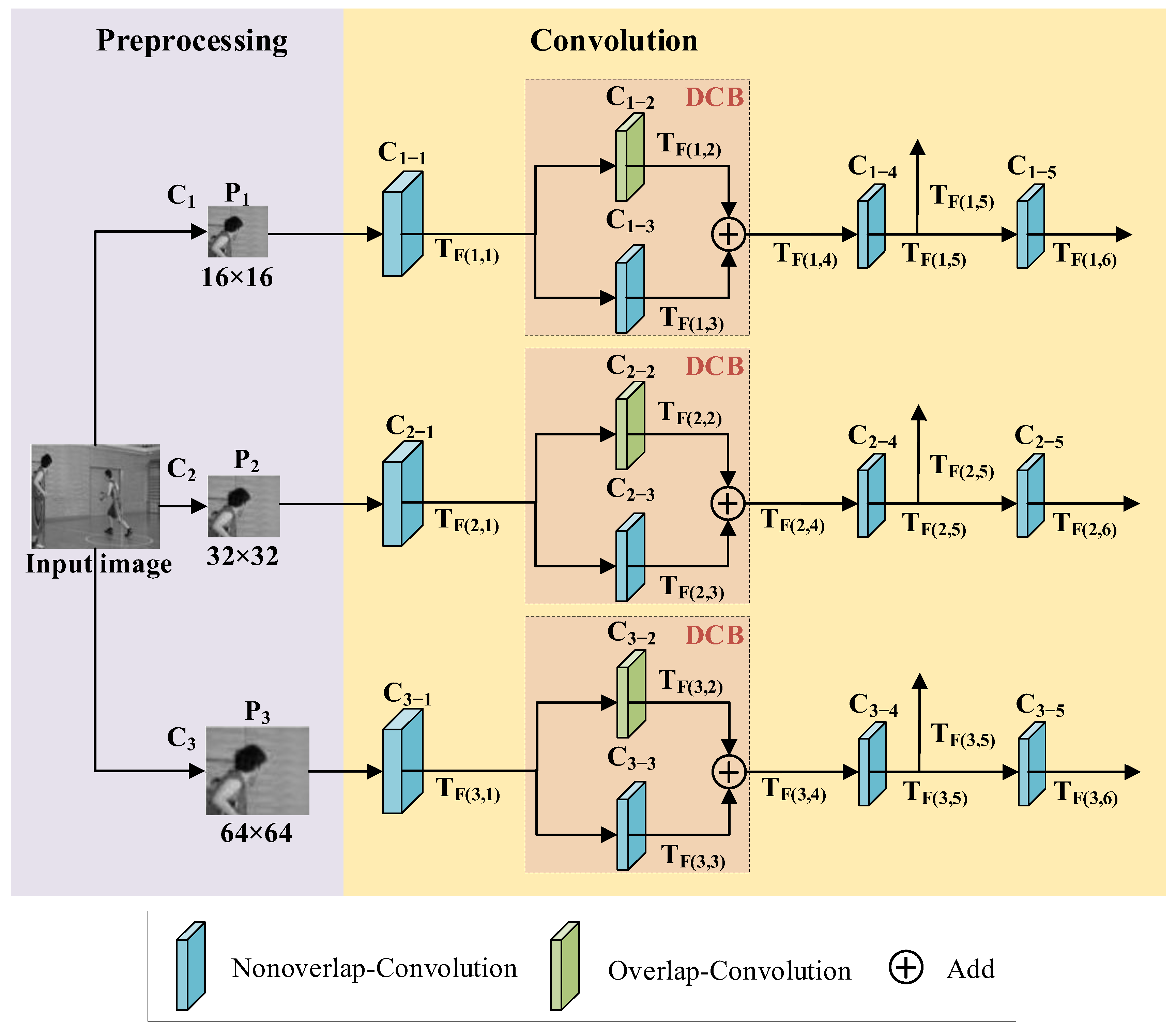
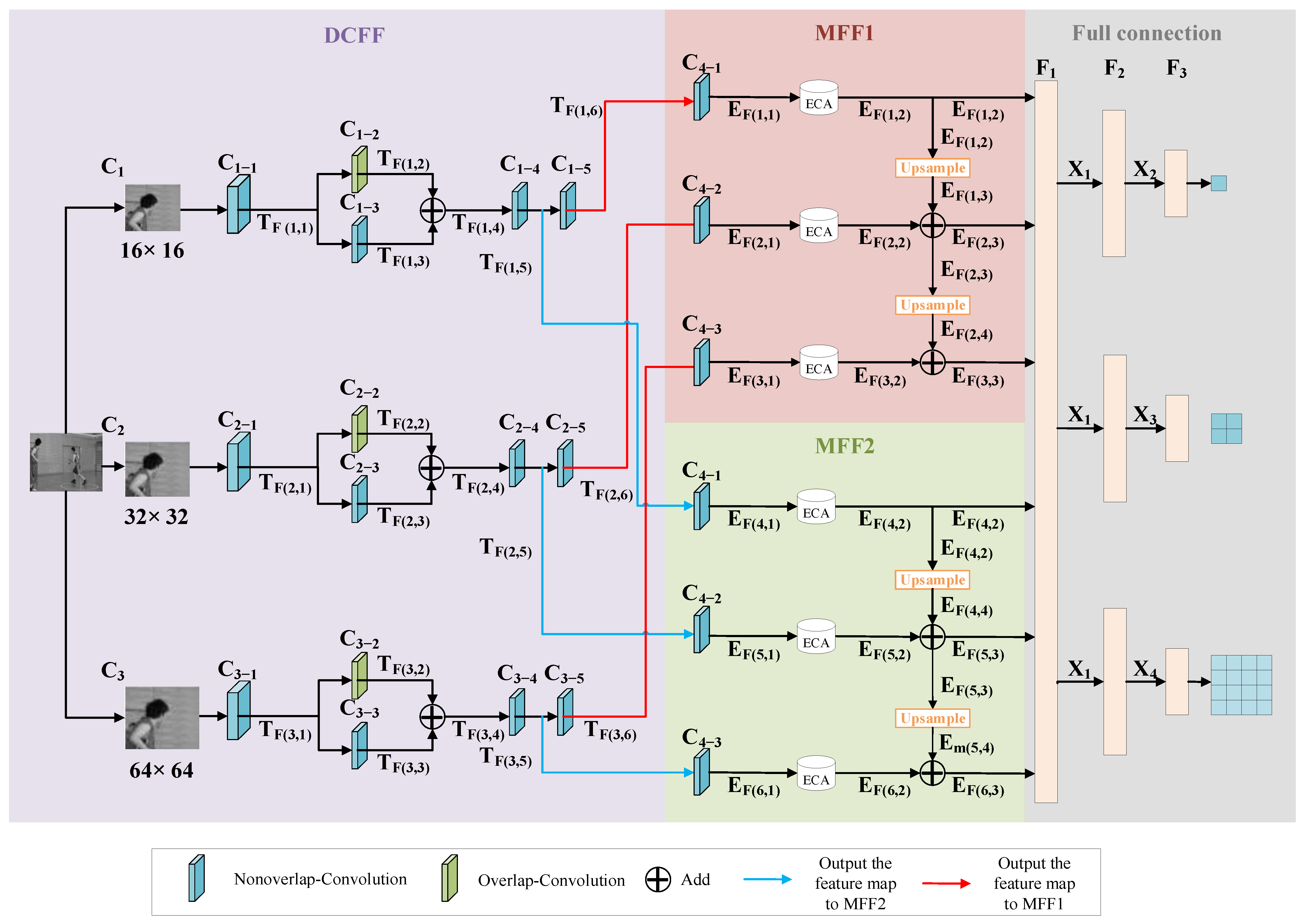
The proposed DCFF (As shown in Figure 1) comprises three branches, namely C₁, C₂, and C₃, which output prediction maps of sizes 16 × 16, 32 × 32, and 64 × 64, correspondingly. After mean removal and downsampling, the input image is converted into a luminance pixel matrix P_i (i = 1, 2, 3). Each corresponding branch where P_i (i = 1, 2, 3) is located contains multiple convolutional blocks with different parameters, with the core being a double convolutional block (DCB). It is worth noting that due to the different matrix sizes caused by mapping relationships and downsampling, the convolutional layers in each branch only accept the corresponding preprocessed encoding unit blocks as inputs. This ensures that the size of the feature map T_F(i,j) (i = 1, 2, 3; j = 5, 6) output by each branch is in a proportional scaling relationship, and the edge length is gradually doubled, allowing smooth input into subsequent modules. This design enables the same network architecture to effectively learn features at different scales.

The DCFF begins by performing convolution operations on the P_i (i = 1, 2, 3) of the three branches, generating three feature maps, respectively. C_i−1 (i = 1, 2, 3) extracts low-level features of P_i, respectively, partitioning.

T_F(i,1) = C_i−1(P_i) (i = 1, 2, 3)

(1)

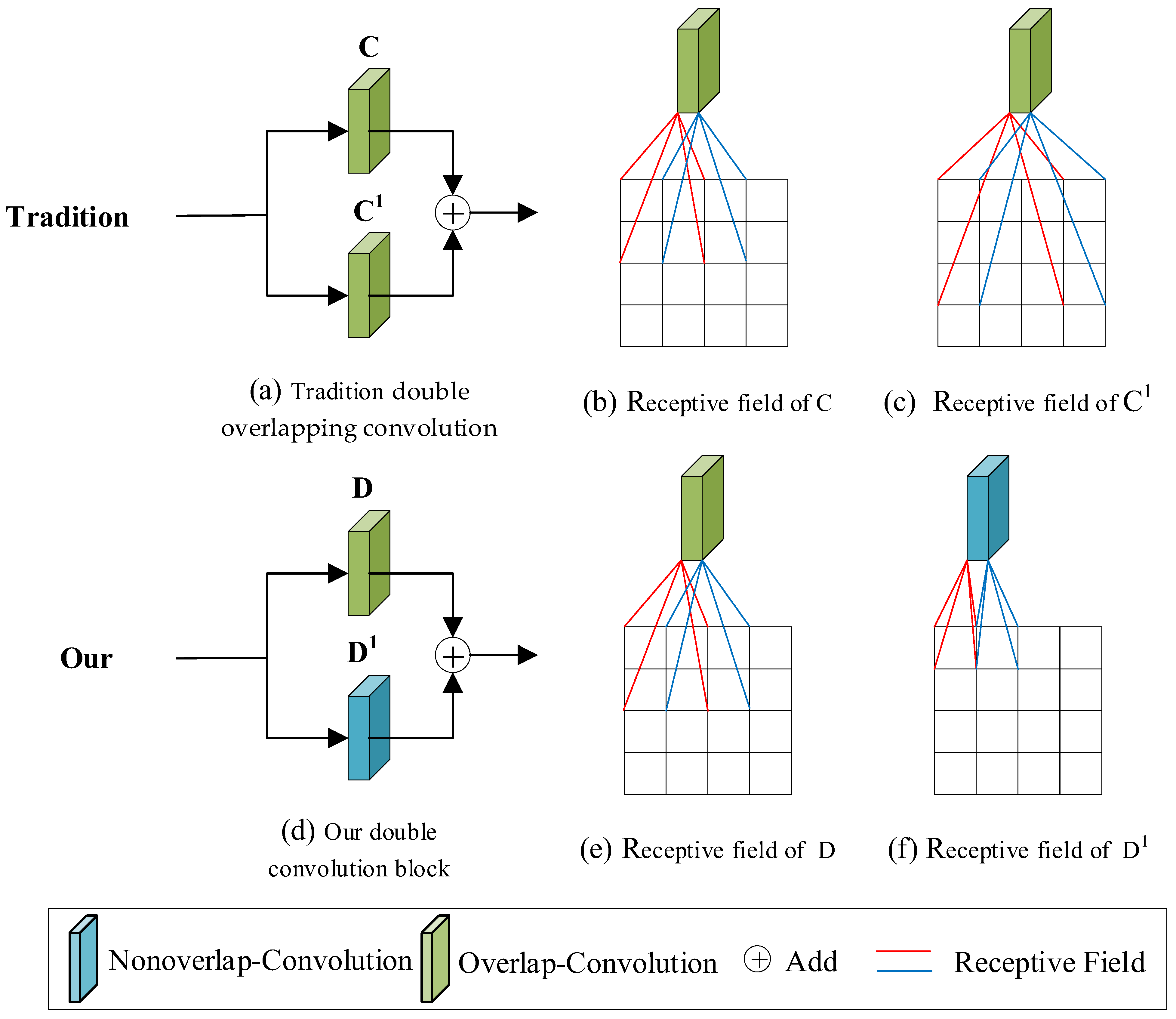
Deep learning-based video encoding usually uses double overlapping convolution to extract features, the detail is illustrated in Figure 2a–c. However, this method leads to high computational overhead and also loses a significant amount of contextual information in the boundary region. Unlike the traditional method, we propose an innovative parallel convolution block called the double convolution block (DCB). The detailed structure is shown in Figure 2. This module applies 2 × 2 overlapping convolution and 1 × 1 non-overlapping convolution to the feature map, and fuses the feature maps obtained by the two convolutions together through element addition, as shown in Figure 2d–f. The uniqueness of this method lies in the fact that overlapping convolution extracts more accurate feature details by utilizing contextual information near the boundary region, thereby improving the accuracy and robustness of convolution. Non-overlapping convolution aligns directly with the non-overlapping partitions of the input feature map, which helps to reduce computational overhead and enhance the model’s generalization ability. In Figure 2, D represents a 2 × 2 overlapping convolution and D¹ represents a 1 × 1 non-overlapping convolution, respectively. In this section, for the non-DCB part, we set the stride of the non-overlapping convolution to be consistent with the size of the kernel. The stride of overlapping convolution in DCB is set to 1, which is the same as that of non-overlapping convolution; the channel is set to 16.

We place the DCB after C_i−1 (i = 1, 2, 3) because useless features are filtered out, but without further feature extraction, a large number of effective features that can be used are preserved. Through the DCB, these features can be maximally learned and fused to generate the feature map T_F(i,2) (i = 1, 2, 3).

T_F(i,4) = DCB(T_F(i,1)) (i = 1, 2, 3)

(2)

Two feature maps T_F(i,j+1) (i = 1, 2, 3; j = 5, 6) on each branch are generated through convolution C_i−j (i = 1, 2, 3; j = 4, 5) to extract high-level features.

T_F(i,j+1) = C_i−j(T_F(i,j)) (i = 1, 2, 3; j = 4, 5)

(3)

The output feature map in Formula (3) above is a fully optimized and refined feature representation that can be used for subsequent processing or decision-making.

By using convolution and DCB modules for processing, the proposed DCFF can not only effectively extract image features but also further optimizes feature representation, reduce information loss, and improve the accuracy and effectiveness of features. The upward arrow marked T_F(i,5) (i = 1, 2, 3) in Figure 1 represents the output of the DCFF, which is then passed to the subsequent MFF module.

Table 1. Parameter configurations for the DCFF.

Branch (i = 1, 2, 3)	Layer (i = 1, 2, 3)	Input (i = 1, 2, 3)	Proposed DCFF Configuration	Output (i = 1, 2, 3)
Ci	Ci−1	Pi	S(16) Conv(4 × 4 × 16)	TF(i,1)
	DCB	TF(i,1)	/	TF(i,4)
	Ci−2	TF(i,4)	S(2) Conv(2 × 2 × 24)	TF(i,5)
	Ci−3	TF(i,5)	S(2) Conv(2 × 2 × 32)	TF(i,6)

lists the detailed parameters, where Conv, S, and T_F represent convolution, stride, and the feature map of the DCFF, respectively.

2.2. Multi-Scale Feature Fusion Module

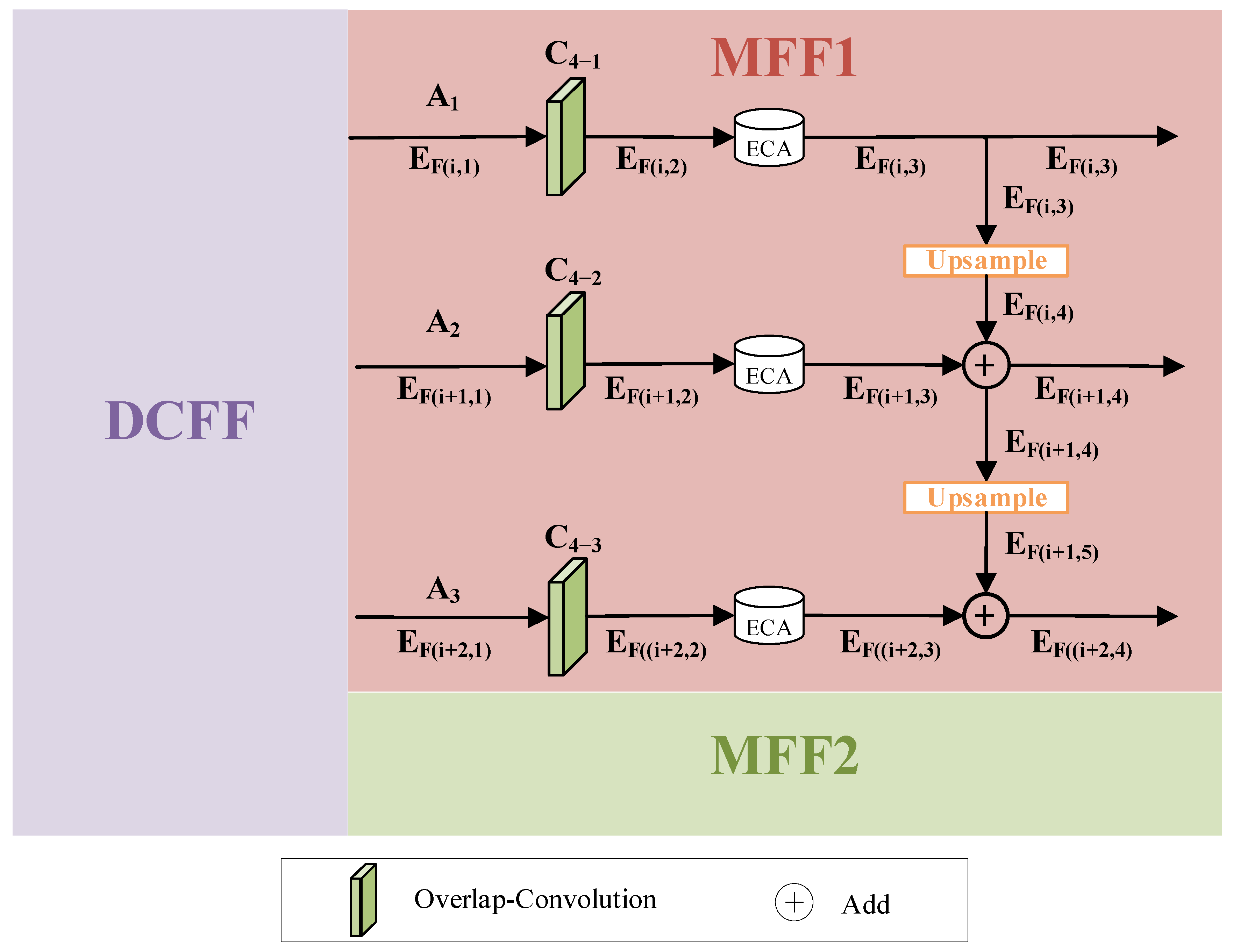
The traditional feature fusion methods usually have drawbacks such as loss of details, identical requirements for feature map size and channel count, and increased computational overhead. To this end, this paper innovatively combines attention mechanism with convolution and proposes a new feature fusion module called MFF module. This module is used repeatedly as a whole within the architecture, as shown in Figure 3. By integrating channel features and multi-scale feature maps through Upsample and feature map add operations, this module not only enhances information exchange but also significantly improves network performance. In order to extract features more effectively, this paper adopts two MFF modules, which have the same structure but differ in the size of their input and output feature maps.

The MFF module employs a three-branch parallel structure design, namely the low-level feature branch A₃, the middle-level feature branch A₂, and the high-level feature branch A₁, which correspond to the three branches of DCFF mentioned. Firstly, the input feature map E_F(v,1) (v = i, i + 1, i + 2) of the module is passed through the convolutional layer C_4−j (j = 1, 2, 3) to output the feature map E_F(v,2) (v = i, i + 1, i + 2). This step uses 1 × 1 convolution, which serves two main purposes: on one hand, it maintains the full spatial structure of the feature map, preventing the loss of spatial information induced by downsampling operations; on the other hand, it performs cross-channel weighted combination by learning the contribution weights of different input channels to the output channels, ultimately achieving cross-channel information fusion.

Secondly, the efficient channel attention (ECA) [27] can effectively capture long-range dependencies between channels and solve the problem of information loss caused by dimensionality reduction by adopting a local cross-channel interaction strategy. Therefore, this paper uses ECA to restore details that are lost during feature extraction. The feature map E_F(v,2) (v = i, i + 1, i + 2) is recalibrated through attention mechanisms to generate feature maps E_F(v,3) (v = i, i + 1, i + 2) with channel and spatial attention weights. It can adaptively highlight important features and suppress redundant features.

E_F(v,3) = ECA(C_4−j(E_F(v,1))) (j = 1, 2, 3; v = i, i + 1, i + 2)

(4)

Finally, a progressive multi-scale feature fusion strategy is adopted for feature fusion. The features of the higher-level branch are divided into two sub-branches, one of which outputs directly, and the other branch is upsampled and then fused with the features of the lower-level branch through element-wise summation to gain the final feature map of the lower level after fusing high-level semantic features. As mentioned in Section 2.1, due to the different multi-scales of the input images in the three branches, the output feature maps of each branch not only have different sizes, but also have certain differences in the details of the extracted texture features. Our method of fusing features from different branches can effectively eliminate the impact of shallow feature maps lacking semantics and deep feature maps lacking details caused by multi-layer convolution extraction, thus achieving cross-level feature complementarity while maintaining feature dimension consistency and improving the overall performance of MFF modules.

E_F(v+1,4) = Upsample(E_F(v,v+2))+E_F(v+1,3) (v = i, i + 1)

(5)

The low-resolution features output by deep networks usually contain rich semantic information but lack spatial details, while the high-resolution features generated by shallow networks retain fine spatial structure despite lower semantic abstraction. The bottom-up feature fusion method we proposed achieves progressive integration of multi-scale features, which can simultaneously utilize the advantages of different levels of representation and effectively make up for the inevitable fine-grained detail loss throughout the network layer by layer, so that the features at each level complement and enhance each other. In addition, the collaborative operation of the 1 × 1 convolutional layer and attention mechanism has produced significant synergistic effects: in the audio and video domains encoding and decoding, the 1 × 1 convolutional layer enhances the compatibility of different modal features through cross-channel transformation, enabling the network to better handle heterogeneous data; The attention mechanism establishes a precise channel weight allocation mechanism, allowing the model to adaptively focus on task-related feature channels. This architectures design achieves a significant improvement in feature representation capability while maintaining computational efficiency.

The specific parameter configuration of the MFF module is detailed in

Table 2. Parameter configurations for the MFF module.

Branch	Layer	Input	Proposed MFF Module Configuration	Output
A1	C4−1	EF(i,1)	S(1) Conv(1 × 1 × 32)	EF(i,2)
	Attention	EF(i,2)	/	EF(i,3)
	Upsample	EF(i,3)	SF = 2	EF(i,4)
A2	C4−2	EF(i+1,1)	S(1) Conv(1 × 1 × 32)	EF(i+1,2)
	Attention	EF(i+1,2)	/	EF(i+1,3)
	Add	EF(i,4),EF(i+1,3)	/	EF(i+1,4)
	Upsample	EF(i+1,4)	SF = 2	EF(i+1,5)
A3	C4−3	EF(i+2,1)	S(1) Conv(1 × 1 × 32)	EF(i+2,2)
	Attention	EF(i+2,2)	/	EF(i+2,3)
	Add	EF(i+1,5),EF(i+2,3)	/	EF(i+2,4)

, where convolution, stride, scale factor, and feature map are respectively referred to as Conv, S, SF, and E_F.

2.3. DCMFF-Net Architecture

The proposed DCMFF-Net architecture, illustrated in Figure 4, mainly consists of three parts: DCFF, MFF module, and three fully connected layers. Our DCMFF-Net consists of three branches, namely C₁, C₂, and C₃, corresponding to different sizes of the input image. Each branch sequentially passes the preprocessed input image information through our designed DCFF, MFF module, and fully connected layer to obtain the final decision.

Specifically, DCFF firstly, it is convolved through C_1−j (j = 1, 2, 3), then through DCB, and finally through C_i−j (i = 4, 5; j = 1, 2, 3) convolutions.

The feature map T_F(i,5) (i = 1, 2, 3) output from C_i−4 (i = 1, 2, 3) is sent to the first MFF module (MFF1). The feature map T_F(i,6) (i = 1, 2, 3) output from C_i−5 (i = 1, 2, 3) is input in the same order to a second MFF module (MFF2) for feature fusion. The main reason why we use MFF1 and MFF2 at different locations is to obtain more effective features and better recover the information loss in feature extraction.

The final part of the DCMFF-Net is the full connection layer. The main function of this layer is to connect all the scattered, high-dimensional features output by DCB and perform a weighted combination. It can learn the complex relationships between these different features and the varying importance of these features. In F₁, the fused feature map E_F(i,2) (i = 1, 4), E_F(i,3) (i = 2, 3, 5, 6) output by MFF is firstly mapped and converted into a one-dimensional vector, which is concatenated and finally output as X₁. This one-dimensional feature vector comprises all of the critical information output by the extraction module. These features are extracted and fused through a carefully designed DCFF and MFF module, which can effectively preserve important information in the input data and provide strong support for subsequent classification or decision-making tasks. Secondly, X₁ is input into each branch of the fully connected layer F₂, which is used to predict whether feature maps of different sizes will be partitioned. After further nonlinear transformation and feature extraction, the output is a new vector X_n (n = 2, 3, 4). This process further enhances the expressive power of features, thus better capturing complex patterns and relationships. Finally, after being processed by the fully connected layer, the texture complexity of the current image region is determined, and the probability of dividing the image region is obtained to decide whether the present image region requires partitioning.

Table 3. Parameter configurations for the DCMFF-Net.

Branch	Layer	Proposed DCMFF-Net Configuration		Output Size
	C1-1	S(4) Conv(4 × 4 × 16)		4 × 4 × 16
	C1-2	S(1) Conv(2 × 2 × 16)		4 × 4 × 16
C1	C1-3	S(1) Conv(1 × 1 × 16)		4 × 4 × 16
	C1-4	S(2) Conv(2 × 2 × 24)		2 × 2 × 24
	C1-5	S(2) Conv(2 × 2 × 32)		1 × 1 × 32
	C2-1	S(4) Conv(4 × 4 × 16)		8 × 8 × 16
	C2-2	S(1) Conv(2 × 2 × 16)		8 × 8 × 16
C2	C2-3	S(1) Conv(1 × 1 × 16)		8 × 8 × 16
	C2-4	S(2) Conv(2 × 2 × 24)		4 × 4 × 24
	C2-5	S(2) Conv(2 × 2 × 32)		2 × 2 × 32
	C3-1	S(4) Conv(4 × 4 × 16)		16 × 16 × 16
	C3-2	S(1) Conv(2 × 2 × 16)		16 × 16 × 16
C3	C3-3	S(1) Conv(1 × 1 × 16)		16 × 16 × 16
	C3-4	S(2) Conv(2 × 2 × 24)		8 × 8 × 24
	C3-5	S(2) Conv(2 × 2 × 32)		4 × 4 × 32
MFF1	C4-1	S(1) Conv(1 × 1 × 32)		1 × 1 × 32
	Attention	/		1 × 1 × 32
	C4-2	S(1) Conv(1 × 1 × 32)		2 × 2 × 32
	Attention	/		2 × 2 × 32
	C4-3	S(1) Conv(1 × 1 × 32)		4 × 4 × 32
	Attention	/		4 × 4 × 32
MFF2	C4-1	S(1) Conv(1 × 1 × 24)		2 × 2 × 24
	Attention	/		2 × 2 × 24
	C4-2	S(1) Conv(1 × 1 × 24)		4 × 4 × 24
	Attention	/		4 × 4 × 24
	C4-3	S(1) Conv(1 × 1 × 24)		8 × 8 × 24
	Attention	/		8 × 8 × 24
Fully Connection		C1	C2	C3
	F1	64	128	256
	F2	48	96	192
	F3	1	4	16

lists the detailed parameter configuration information of DCMFF-Net.

To gain deeper insight into the relationship between neural network output feature maps and CU partitioning in actual encoding, we have provided the following explanation:

According to the HEVC standard, a CTU consists of four CU dimensions: 64 × 64, 32 × 32, 16 × 16, and 8 × 8, corresponding to indices i = 0, 1, 2, and 3, where i represents the depth level.

HEVC commonly uses S_i (i = 0, 1, 2, 3) to determine whether the current CU is divided, where i represents which layer the current CU is located in: S_i = 0 indicates no partitioning and S_i = 1 indicates that partitioning will occur. Specifically, S_i (i = 0) at the CTU level is represented by a single label. S_i (i = 1) at the CTU level is represented by four labels. S_i (i = 2) at the CTU level is represented by sixteen labels. For S_i (i = 3), no additional decision labels are required, as its partitioning is determined by the previously defined S_i (i = 0, 1, 2) labels.

Thus, each CTU contains a total of 21 partitioning decisions (1 + 4 + 16 = 21). These decision flags are used to describe the CU partitioning structure. Based on this discussion, we categorize the decision labels into three hierarchical levels and apply them in the proposed DCMFF-Net architecture.

Without affecting the generality, this article centers on analyzing the brightness information in video sequences, extracting pixel blocks built from the luminance (Y) components of the input 64 × 64 CTU. In addition, to enhance the convergence of the training data, a global normalization preprocessing step was applied.

After DCMFF-Net, we obtained 21 probabilities and divided them into three layers, representing the probability of QT segmentation during the process of dividing CU from a size of 64 × 64 to the smallest CU. The first, second, and third layers correspond to 1, 4, and 16 probabilities, respectively. These CUs correspond to a total of 21 different decision outputs. These outputs are processed using the Sigmoid activation function, mapping the output values to the (0, 1) interval to obtain the probability values of each decision output, which facilitates subsequent classification or decision operations. In addition, to enhance the adaptability of CU partition prediction to different quantization parameter (QP) values, QP values are merged as additional features into the fully connected layers F₂ and F₃. In this way, the network can better adjust its prediction strategy based on different quantization parameters, thereby improving the robustness and accuracy of the network under different encoding conditions.

2.4. Loss Function

Since a classification task essentially involves predicting a probability distribution, the cross-entropy loss function is ideal as it directly measures the difference between two probability distributions. Moreover, the loss function we use is a convex function, meaning it has only one global minimum and no local minimum, which can make our optimization process more stable and efficient. Therefore, we choose the cross-entropy loss function for our work. Assuming we have S training samples, the predicted values from branches C₁, C₂, and C₃ are denoted as ${\{{\mathrm{y}}_{{\mathrm{C}}_1}^{*}\left(\mathrm{t}\right)\}}_{\mathrm{t}=1}^1$, ${\{{\mathrm{y}}_{{\mathrm{C}}_2}^{*}\left(\mathrm{t}\right)\}}_{\mathrm{t}=1}^4$ and ${\{{\mathrm{y}}_{{\mathrm{C}}_3}^{*}\left(\mathrm{t}\right)\}}_{\mathrm{t}=1}^{16}$ with their corresponding ground truth labels represented as ${\{{\mathrm{y}}_{{\mathrm{C}}_1}\left(\mathrm{t}\right)\}}_{\mathrm{t}=1}^1$, ${\{{\mathrm{y}}_{{\mathrm{C}}_2}\left(\mathrm{t}\right)\}}_{\mathrm{t}=1}^4$ and ${\{{\mathrm{y}}_{{\mathrm{C}}_3}\left(\mathrm{t}\right)\}}_{\mathrm{t}=1}^{16}$. The loss function ${\mathrm{L}}_{\mathrm{s}}$ is given by

$${\mathrm{L}}_{\mathrm{s}}=\sum _{\mathrm{t}=1}^1(\mathrm{H}({\mathrm{y}}_{{\mathrm{C}}_1}(\mathrm{t}),{\mathrm{y}}_{{\mathrm{C}}_1}^{\mathrm{*}}(\mathrm{t}))+\sum _{\mathrm{t}=1}^4(\mathrm{H}({\mathrm{y}}_{{\mathrm{C}}_2}(\mathrm{t}),{\mathrm{y}}_{{\mathrm{C}}_2}^{\mathrm{*}}(\mathrm{t}))+\sum _{\mathrm{t}=1}^{16}(\mathrm{H}({\mathrm{y}}_{{\mathrm{C}}_3}(\mathrm{t}),{\mathrm{y}}_{{\mathrm{C}}_3}^{\mathrm{*}}(\mathrm{t}))$$

(6)

$$\mathrm{L}={\displaystyle \frac{1}{\mathrm{S}}}{\sum }_{\mathrm{s}=1}^{\mathrm{S}}\left({\mathrm{L}}_{\mathrm{s}}\right)$$

(7)

Among them, H (*) is the cross-entropy operator between the real label and the predicted label.

2.5. Proposed DCMFF-Net Flowcharts

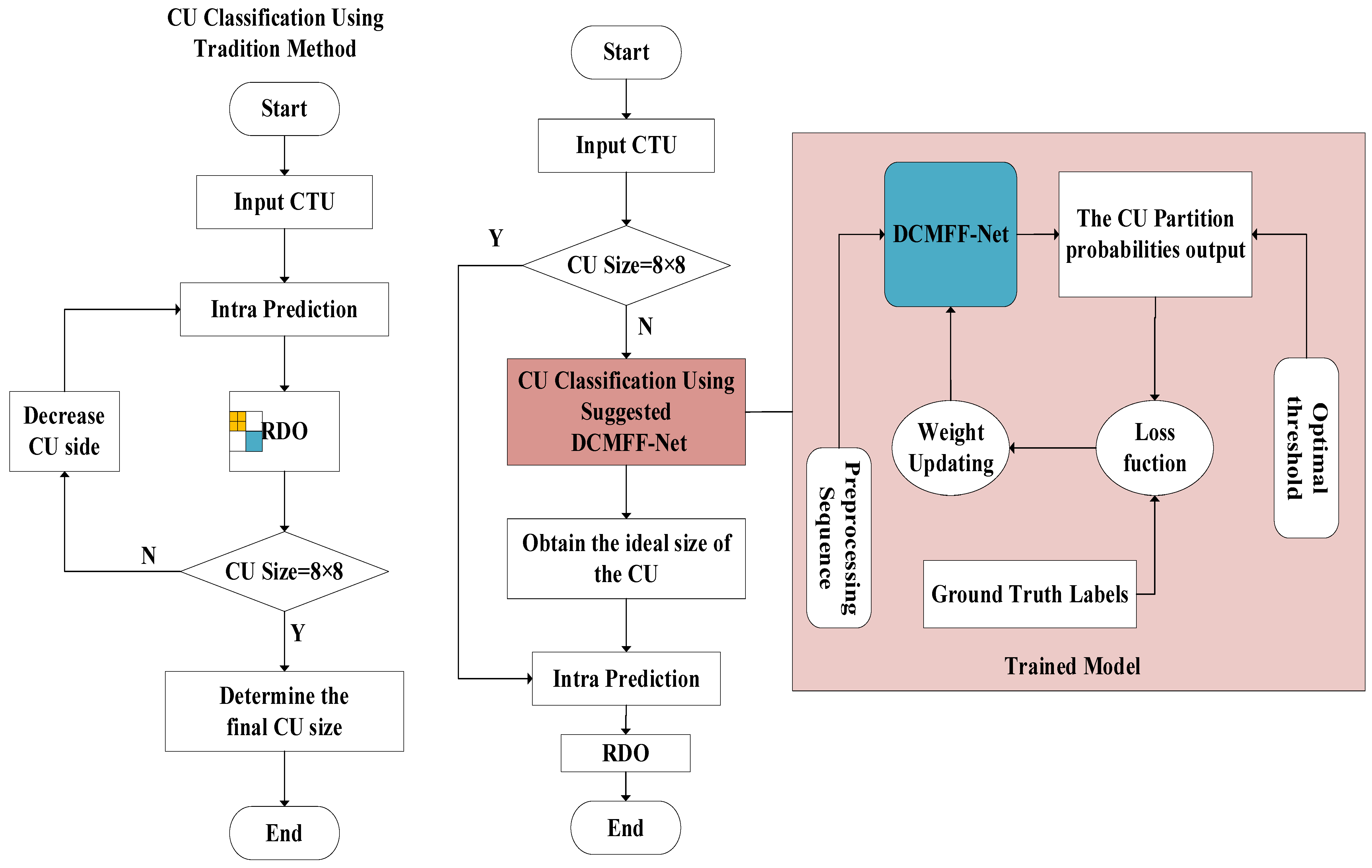
The workflow of embedding DCMFF-Net into the encoder appears in Figure 5. The entire encoding process comprises two fundamental components: (1) training the DCMFF-Net to generate models for CUs segmentation labels in images. (2) Replace the RDO exhaustive algorithm and use the trained model to predict CU segmentation. Compared with traditional CU classification methods, this approach can avoid unnecessary RDO redundant calculations. The DCFF proposed in this article effectively extracts fine feature details, while the MFF module significantly enhances sequence feature extraction and fusion. Ultimately, these two modules work together to construct DCMFF-Net for predicting CU partitions.

Moreover, we have implemented an early stopping mechanism to effectively curtail unnecessary CU partitioning and encoding steps. Specifically, if the first-level decision determines that there are no partitions, the second- and third-level partitioning processes will be skipped. If the second-level decision indicates no further partitioning, the third-level partitioning process is also omitted.

3. Experimental Setup

3.1. Experimental Parameter Configuration

The specific configuration and evaluation criteria are detailed below: This study employs the HEVC benchmark HM16.5 as its experimental platform, with videos encoded at four QP values: {22, 27, 32, 37}. The CPHI Test Set [28] with images of various resolutions is used for training. This dataset contains a total of 2000 images with a resolution of 4928 × 3264. After preprocessing, the dataset is randomly split into three subsets: an 85% training set, a 10% testing set, and a 5% validation set. Each subset is further divided into four equal groups, each corresponding to a different resolution. To generate the final training, testing, and validation datasets with CU division labels, all images are encoded using HM16.5 at the four QP values, ensuring that the datasets contain sufficient and diverse CU partitioning information.

The training phase utilized an NVIDIA GeForce GTX 1650 GPU-accelerated mode, whereas testing tasks were executed on an Intel i7 CPU platform. GPU acceleration was restricted to model optimization procedures and remained inactive during testing.

The configuration file encoder_intra_main.cfg [18] was used to evaluate the modes. The network framework was implemented using TensorFlow1.15. During model training, all trainable parameters were randomly initialized. The model’s initial learning rate (η) was configured as 0.01, with the batch size parameter defined at n = 64, and executed over 1,000,000 optimization steps.

3.2. Performance Evaluation Metrics and Test Sequence Parameters

To effectively express the predictive performance of the designed DCMFF-Net, Validation experiments were conducted by encoding 18 standard sequences derived from five distinct resolutions, following a fair comparison protocol as established by JCT-VC [29]. The sequences are classified into five categories (A–E), with all settings based on the default configurations of the Common Test Conditions (CTCs), which are detailed in

Table 4. Test sequence parameters. (There are 5 types of test sequences (A–E), each with different video scenes).

Class	Sequence	Resolution	Length (S)	Frame Rate (HZ)	Number Frames
A	People On Street	2560 × 1600	5	30	150
	Traffic	2560 × 1600	5	30	150
B	Basketball Drive	1920 × 1080	10	50	500
	BQ Terrace	1920 × 1080	10	60	600
	Cactus	1920 × 1080	10	50	500
	Kimono	1920 × 1080	10	24	240
	Park Scene	1920 × 1080	10	24	240
C	Basketball Drill	832 × 480	10	50	500
	BQ Mall	832 × 480	10	60	600
	Party Scene	832 × 480	10	50	500
	Race Horses	832 × 480	10	30	300
D	Basketball Pass	416 × 240	10	50	500
	Blowing Bubbles	416 × 240	10	50	500
	BQ Square	416 × 240	10	60	600
	Race Horses	416 × 240	10	30	300
E	Four People	1280 × 720	10	60	600
	Johnny	1280 × 720	10	60	600
	Kriten And Sara	1280 × 720	10	60	600

. Additionally, the evaluation metrics used in our paper are based on VCEG-M33 [30] standards, including ∆T, BD-BR, and BD-PSNR: ∆T indicates the percentage of encoding time saved against the HM16.5. Evaluation of the image quality of encoding sequence was performed using BD-BR and BD-PSNR, where BD-BR reflects the average bitrate difference between our algorithm and the original encoding algorithm. BD-PSNR indicates the average PSNR difference. The formula is expressed as follows:

$$∆\mathrm{T}({\mathrm{QP}}_{\mathrm{i}}) = {\displaystyle \frac{{\mathrm{T}}_{\mathrm{p}\mathrm{r}\mathrm{o}\mathrm{p}\mathrm{o}\mathrm{s}\mathrm{e}\mathrm{d}}\left({\mathrm{QP}}_{\mathrm{i}}\right)- {\mathrm{T}}_{\mathrm{H}\mathrm{M}}\left({\mathrm{QP}}_{\mathrm{i}}\right)}{{\mathrm{T}}_{\mathrm{HM}}\left({\mathrm{QP}}_{\mathrm{i}}\right)}} \times 100\%$$

(8)

$$∆\mathrm{T}={\displaystyle \frac{1}{4}} \sum _{\mathrm{i}=1}^4∆\mathrm{T}\left({\mathrm{QP}}_{\mathrm{i}}\right)\times 100\%$$

(9)

where THM and Tproposed represent the encoding time of the HM16.5 and the encoding time using the DCMFF-Net, respectively. During encoding, the QP values are selected from {22, 27, 32, 37}. BD-PSNR reflects the residual error between the original and reconstructed pixels, and its calculation formula is as follows:

BD-PSNR = PSNR_proposed − PSNR_HM

(10)

where PSNR_proposed and PSNR_HM represent the average PSNR of the introduced algorithm and the source encoder, respectively. BD-BR denotes the average bitrate difference between the source algorithm and the proposed method:

$$\mathrm{BD}-\mathrm{BR} = {\displaystyle \frac{{\mathrm{B}\mathrm{D}-\mathrm{R}\mathrm{a}\mathrm{t}\mathrm{e}}_{\mathrm{p}\mathrm{r}\mathrm{o}\mathrm{p}\mathrm{o}\mathrm{s}\mathrm{e}\mathrm{d}}-{\mathrm{B}\mathrm{D}-\mathrm{R}\mathrm{a}\mathrm{t}\mathrm{e}}_{\mathrm{H}\mathrm{M}}}{{\mathrm{B}\mathrm{D}-\mathrm{R}\mathrm{a}\mathrm{t}\mathrm{e}}_{\mathrm{H}\mathrm{M}}}} \times 100\%$$

(11)

where BD-Rate_proposed and BD-Rate_HM represent the average bitrate of the introduced algorithm and the average bitrate of the source encoder, respectively.

3.3. Ablation Experiments

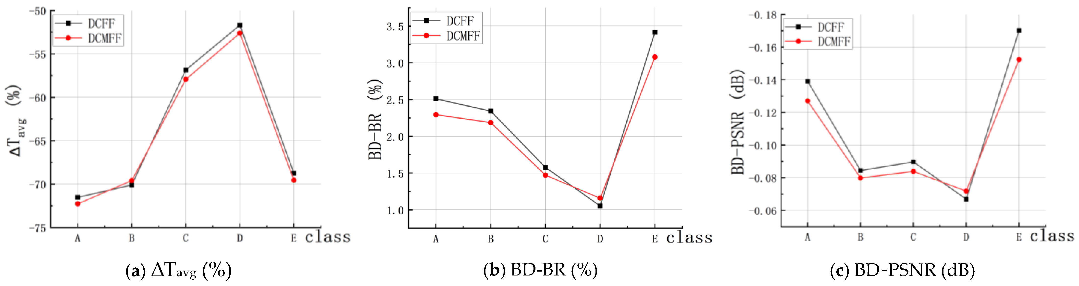
To evaluate the DCMFF-Net and DCFF methods, two ablation experiments were designed. These experiments utilized the first 20 frames of each sequence under identical configurations and four QP levels. As illustrated in Figure 6, the dot markers indicate the averaged results across five sequences (A–E) for each QP setting.

From Figure 6, it can be observed that DCMFF-Net achieves a better overall balance in coding efficiency compared to the DCFF alone, showing varying degrees of enhancement in most cases. This improvement is attributed to the proposed MFF module, which possesses strong feature extraction and fusion capabilities, helping to preserve details in the feature maps and improve prediction accuracy. Moreover, the high compatibility between the various modules enhances the overall representational ability of DCMFF-Net. These results confirm that incorporating the MFF module enhances the representational capacity of the network, leading to superior performance across most evaluated metrics.

3.4. RD Performance Evaluation

As

Table 5. The test results of A-E sequence in JCT-VT of our proposed method.

Class	Sequence	BD-BR (%)	BD-PSNR (dB)	∆T(%)
				QP = 22	QP = 27	QP = 32	QP = 37
A (2560 × 1600)	People On Street	2.15	−0.12	−74.32	−73.94	−74.95	−74.28
	Traffic	2.43	−0.13	−75.59	−65.45	−68.22	−71.37
	Average Class A	2.29	−0.12	−74.96	−69.70	−71.59	−72.82
B (1920 × 1080)	Basketball Drive	4.10	−0.10	−70.36	−75.44	−77.45	−79.21
	BQ Terrace	1.18	−0.07	−52.31	−55.55	−57.85	−60.32
	Cactus	2.02	−0.07	−54.06	−61.68	−65.23	−69.49
	Kimono	1.72	−0.06	−83.36	−83.47	−83.65	−84.06
	Park Scene	1.89	−0.08	−61.40	−64.90	−73.40	−78.72
	Average Class B	2.18	−0.07	−64.30	−68.21	−71.52	−74.36
C (832 × 480)	Basketball Drill	2.75	−0.13	−41.31	−48.21	−58.26	−66.48
	BQ Mall	1.16	−0.07	−45.97	−50.97	−52.86	−56.47
	Party Scene	0.32	−0.02	−55.83	−55.34	−58.22	−61.12
	Race Horses	1.64	−0.10	−65.67	−67.30	−69.03	−72.94
	Average Class C	1.47	−0.08	−52.20	−55.46	−59.59	−64.26
D (416 × 240)	Basketball Pass	2.47	−0.14	−51.54	−55.54	−59.85	−64.93
	Blowing Bubbles	0.79	−0.04	−36.25	−38.87	−46.06	−52.60
	BQ Square	0.30	−0.02	−36.88	−41.96	−44.10	−46.95
	Race Horses	1.05	−0.07	−64.83	−66.49	−66.23	−69.10
	Average Class D	1.15	−0.07	−47.38	−50.72	−54.06	−58.40
E (1280 × 720)	Four People	2.63	−0.15	−59.71	−62.22	−64.22	−68.19
	Johnny	3.42	−0.14	−71.52	−72.30	−74.13	−76.21
	Kriten And Sara	3.17	−0.16	−69.03	−70.47	−72.49	−74.07
	Average Class E	3.07	−0.15	−66.75	−68.33	−70.28	−72.82
Average Class A–E		1.95	−0.09	−59.44	−61.67	−64.79	−68.14

indicates, the method used in this study significantly reduced the encoding complexity of four different QP values, while the quality decline of the sequence was minimal. Compared to the source encoder HM16.5, the introduced algorithm reduces encoding time by 58.10% at QP = 22, 61.30% at QP = 27,64.10% at QP = 32, and 67.63% at QP = 37. At the same time, although there is a slight rise in BD-BR (1.95%), the reduction in BD-PSNR is very minimal (only 0.09 dB). Furthermore, the analysis reveals that as the QP value increases, the network architecture we designed becomes more effective in reducing the HEVC encoding time. This improvement is attributed to the DCMFF-Net deep convolutional neural network, which efficiently leverages features and effectively fuses multi-scale feature maps from the three branches, thereby enhancing prediction accuracy. The subtle changes in BD-BR and BD-PSNR further demonstrate that the impact of our approaches on video quality and bitrate has always been within an acceptable range for humans.

To better highlight the contributions of this study, three representative intra-frame encoding methods were selected for comparative analysis using 18 standard video sequences provided by JCT-VC, illustrated in

Table 6. Comparison results of this algorithm with other algorithms on A–E sequences in JCT-VT.

Sequence	[18]			[8]			[31]			Our
	BD- BR (%)	BD- PSNR (dB)	$∆{\mathbf{T}}_{\mathbf{avg}}$ (%)	BD-BR (%)	BD- PSNR (dB)	$∆{\mathbf{T}}_{\mathbf{avg}}$ (%)	BD-BR (%)	BD- PSNR (dB)	$∆{\mathbf{T}}_{\mathbf{avg}}$ (%)	BD-BR (%)	BD- PSNR (dB)	$∆{\mathbf{T}}_{\mathbf{avg}}$ (%)
People On Street	2.37	−0.13	−61.00	1.77	−0.10	−53.34	2.84	−0.15	−57.56	2.15	−0.12	−74.37
Traffic	2.55	−0.13	−70.79	2.38	−0.12	−58.51	2.64	−0.13	−65.53	2.43	−0.13	−70.16
Average Class A	2.46	−0.13	−65.90	2.08	−0.11	−55.93	2.74	−0.14	−61.55	2.29	−0.12	−72.27
Basketball Drive	4.27	−0.12	−76.32	2.18	−0.06	−57.53	3.91	−0.11	−72.26	4.10	−0.10	−75.61
BQ Terrace	1.84	−0.09	−64.72	1.47	−0.07	−56.21	1.99	−0.09	−58.21	1.18	−0.07	−56.50
Cactus	2.27	−0.08	−60.96	2.20	−0.07	−58.25	2.18	−0.07	−65.95	2.02	−0.07	−62.61
Kimono	2.59	−0.09	−83.53	1.82	−0.06	−67.30	2.84	−0.10	−80.90	1.72	−0.06	−83.64
Park Scene	1.96	−0.08	−67.53	2.35	−0.10	−61.97	2.57	−0.11	−65.09	1.89	−0.08	−69.60
Average Class B	2.59	−0.09	−70.61	2.00	−0.07	−60.25	2.70	−0.10	−68.32	2.18	−0.07	−69.59
Basketball Drill	2.86	−0.13	−52.98	2.06	−0.10	−48.93	2.27	−0.11	−53.75	2.75	−0.13	−53.56
BQ Mall	2.09	−0.11	−58.42	1.37	−0.11	−48.44	0.66	−0.05	−42.83	1.16	−0.07	−51.57
Party Scene	0.66	−0.04	−44.49	2.50	−0.14	−47.77	1.87	−0.10	−60.06	0.32	−0.02	−57.88
Race Horses	1.97	−0.11	−57.12	3.15	−0.17	−56.31	2.31	−0.12	−55.79	1.64	−0.10	−68.73
Average Class C	1.90	−0.10	−53.25	2.27	−0.13	−50.36	1.78	−0.10	−53.11	1.47	−0.08	−57.94
Basketball Pass	1.84	−0.11	−56.42	2.72	−0.15	−54.25	1.52	−0.09	−57.30	2.47	−0.14	−57.88
Blowing Bubbles	0.62	−0.04	−40.54	1.43	−0.09	−46.92	0.64	−0.04	−40.32	0.79	−0.04	−43.44
BQ Square	0.91	−0.07	−45.82	1.20	−0.10	−45.47	0.52	−0.04	−46.04	0.30	−0.02	−42.47
Race Horses	1.32	−0.08	−55.75	/	/	/	1.45	−0.08	−52.01	1.05	−0.07	−66.66
Average Class D	1.17	−0.08	−49.63	1.78	−0.11	−48.88	1.03	−0.06	−48.92	1.15	−0.07	−52.61
Four People	3.11	−0.17	−71.31	2.71	−0.15	−59.89	1.76	−0.10	−64.78	2.63	−0.15	−63.58
Johnny	3.82	−0.15	−70.68	2.48	−0.10	−64.67	2.31	−0.09	−75.44	3.42	−0.14	−73.54
Kriten And Sara	3.46	−0.17	−74.86	3.25	−0.16	−62.36	2.21	−0.11	−73.34	3.17	−0.16	−71.52
Average Class E	3.46	−0.16	−72.28	2.81	−0.14	−62.31	2.09	−0.10	−71.19	3.07	−0.15	−69.55
Average Class A-E	2.25	−0.11	−61.84	2.18	−0.11	−55.77	2.03	−0.09	−60.35	1.95	−0.09	−63.52

.

The comparative data in Table 6 indicates that DCMFF-Net achieves a 63.52% reduction in the complexity of the encoder, surpassing the reductions of 61.84%, 55.77%, and 60.35% achieved by [8,18,31], respectively. Notably, while maintaining the same transmission bitrate, our DCMFF-Net outperforms the other three methods in terms of video quality and complexity cost. Experimental validation demonstrates that the DCMFF-Net exhibits outstanding performance in predicting CU partitions, further confirming that the DCMFF-Net deep convolutional neural network employed in this study can effectively train and learn pixel information from CTUs.

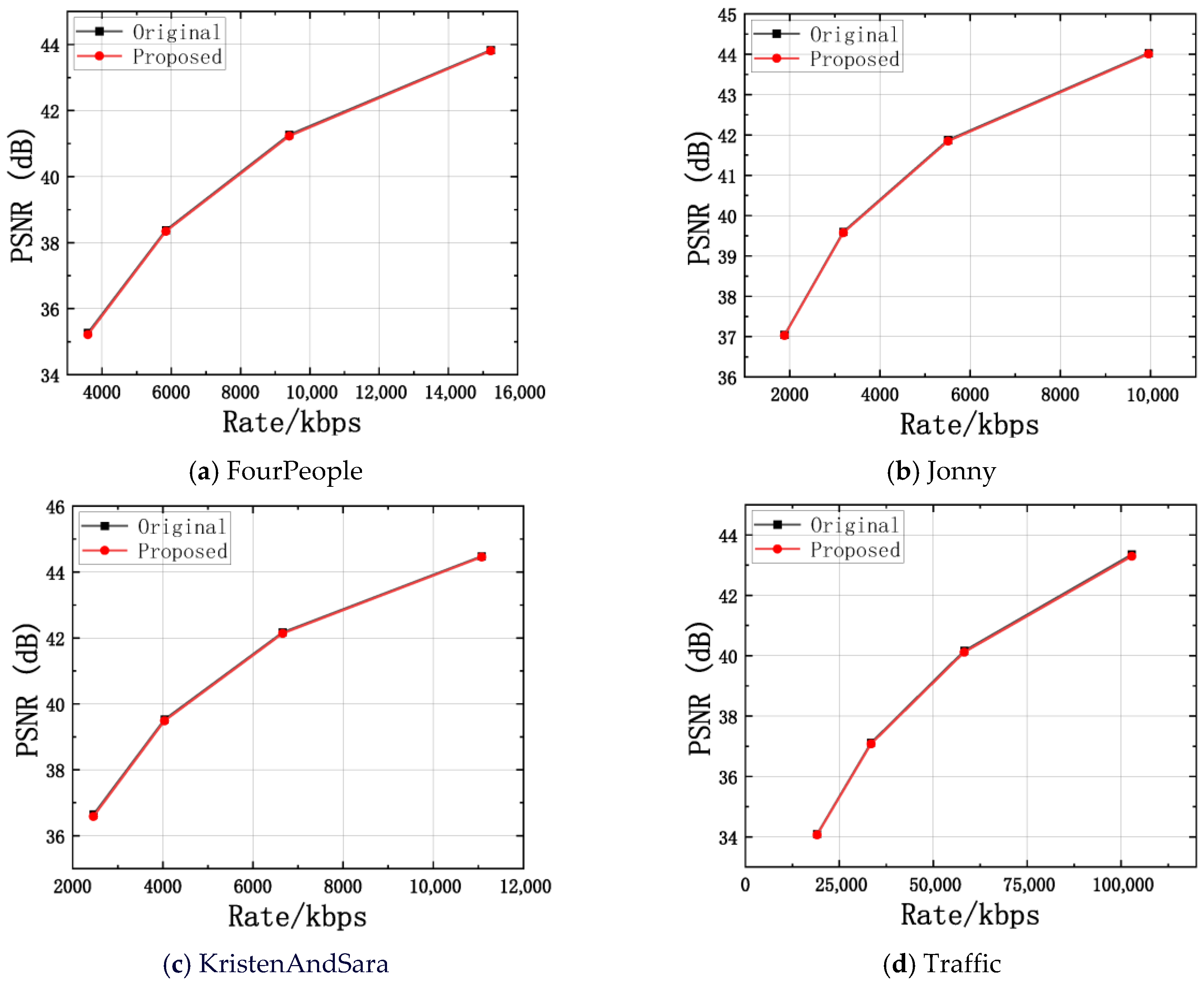
To illustrate the RD performance of our DCMFF-Net, we choose three sequences from Class E—which exhibited the highest average video quality loss—along with the Traffic sequence, which also showed notable quality degradation. The selected sequences are Fourpeople, Jonny, KristenAndSara, and Traffic, and their performance was compared against HM16.5. Figure 7 illustrates the RD performance of these four sequences when encoded using our algorithm and HM16.5. Upon observation, it is evident that the RD curves of the proposed algorithm are very similar to those of the original algorithm, with some curves almost overlapping. This means that our proposed algorithm demonstrates excellent robustness and stability, with video quality loss so minimal that it is virtually negligible compared to the original encoding method.

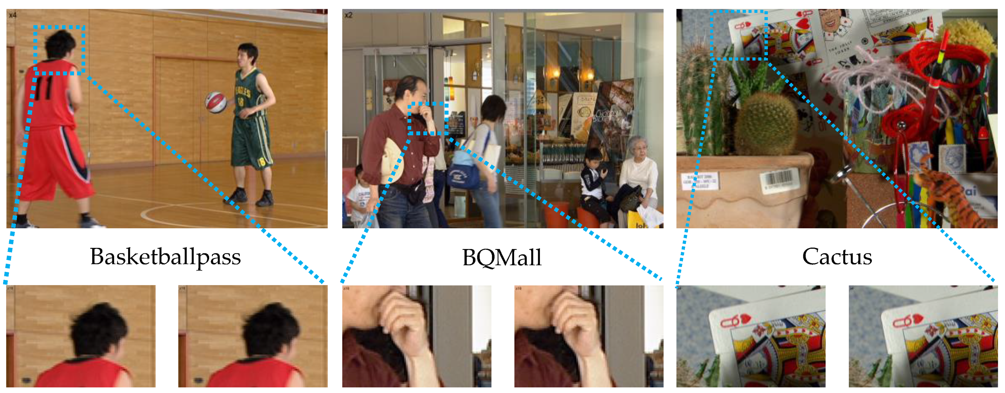
Finally, to assess the subjective performance of our method in this article, we selected I-frames [32] from the BasketballPass, BQMall, and Cactus sequences, containing cluttered environmental contexts and rapidly evolving scenarios. These frames were compared against those encoded using the HM16.5 encoder at QP = 37. Figure 8 presents magnified local detail images of these sequences using our algorithm and HM16 encoding. From the images, it can be observed that the subjective visual perception in the magnified regions is almost indistinguishable between the two algorithms. The image quality variations proposed by the proposed algorithm are below the human visual perception threshold, and thus are negligible. Similar results have also been observed in other JCT-VC test sequences. Therefore, the proposed method demonstrates strong performance in both image quality and encoding efficiency.

4. Conclusions and Outlook

This paper proposes a DCMFF-Net neural network architecture designed to accelerate CU partitioning decisions in intra-frame HEVC video encoding, thereby simplifying the complexity of HEVC. The core contributions include the design and integration of a novel feature fusion module, enabling multi-layer fusion of multi-scale feature maps. Experimental validation demonstrates that the proposed method exhibits outstanding performance and significant advantages. Compared to the traditional HM encoder, the method achieves a 1.95% rise in BD-BR, and a slight reduction in BD-PSNR (0.09 dB) on JCT-VC test sequences, while achieving a 63.52% reduction in encoding complexity.

At the same time, our work still has some limitations, such as the significant impact of inter frame partitioning prediction on encoding complexity in practice. We have not yet completed the relevant work and in the future, we will further reduce complexity by integrating inter frame prediction technology. In addition, we will consider the application of audio and video codec in autonomous vehicles. In this regard, Wiseman [33] has conducted some meaningful explorations, providing us with good reference value. Meanwhile, Racanelli et al. [34] proposed reducing the computational cost of adaptive bit rate controllers from exponential to polynomial levels, which is also a direction we are considering.

References

1. Wiegand, T.; Sullivan, G.J.; Bjontegaard, G.; Luthra, A. Overview of the H.264/AVC video coding standard. IEEE Trans. Circuits Syst. Video Technol. 2003, 13, 560–576. [Google Scholar] [CrossRef] [Scilit]
2. Sullivan, G.J.; Ohm, J.R.; Han, W.J.; Wiegand, T. Overview of the High Efficiency Video Coding (HEVC) Standard. IEEE Trans. Circuits Syst. Video Technol. 2012, 22, 1649–1668. [Google Scholar] [CrossRef] [Scilit]
3. Bross, B.; Wang, Y.K.; Ye, Y.; Liu, S.; Chen, J.; Sullivan, G.J.; Ohm, J.R. Overview of the Versatile Video Coding (VVC) Standard and its Applications. IEEE Trans. Circuits Syst. Video Technol. 2021, 31, 3736–3764. [Google Scholar] [CrossRef] [Scilit]
4. Bossen, F.; Bross, B.; Suhring, K.; Flynn, D. HEVC Complexity and Implementation Analysis. IEEE Trans. Circuits Syst. Video Technol. 2012, 22, 1685–1696. [Google Scholar] [CrossRef] [Scilit]
5. Wu, S.; Shi, J.; Chen, Z. HG-FCN: Hierarchical Grid Fully Convolutional Network for Fast VVC Intra Coding. IEEE Trans. Circuits Syst. Video Technol. 2022, 32, 5638–5649. [Google Scholar] [CrossRef] [Scilit]
6. The Bitmovin. Video Developer Report. Available online: https://go.bitmovin.com/video-developer-report (accessed on 27 November 2018).
7. Shen, L.; Zhang, Z.; Liu, Z. Effective CU Size Decision for HEVC Intracoding. IEEE Trans. Image Process. 2014, 23, 4232–4241. [Google Scholar] [CrossRef] [Scilit] [PubMed]
8. Zhang, Y.; Li, N.; Kwong, S.; Jiang, G.; Zeng, H. Statistical Early Termination and Early Skip Models for Fast Mode Decision in HEVC INTRA Coding. ACM Trans. Multimed. Comput. Commun. Appl. 2019, 15, 70. [Google Scholar] [CrossRef] [Scilit]
9. Lim, K.; Lee, J.; Kim, S.; Lee, S. Fast PU Skip and Split Termination Algorithm for HEVC Intra Prediction. IEEE Trans. Circuits Syst. Video Technol. 2015, 25, 1335–1346. [Google Scholar]
10. Wang, Z.; Bovik, A.C.; Sheikh, H.R.; Simoncelli, E.P. Image Quality Assessment: From Error Visibility to Structural Similarity. IEEE Trans. Image Process. 2004, 13, 600–612. [Google Scholar] [CrossRef] [Scilit]
11. Zhang, Y.; Wang, G.; Tian, R.; Xu, M.; Kuo, C.C.J. Texture-Classification Accelerated CNN Scheme for Fast Intra CU Partition in HEVC. In Proceedings of the 2019 Data Compression Conference, Snowbird, UT, USA, 26–29 March 2019; pp. 241–249. [Google Scholar]
12. Pakdaman, F.; Yu, L.; Hashemi, M.R.; Ghanbari, M.; Gabbouj, M. SVM-based approach for complexity control of HEVC intra coding. Signal Process. Image Commun. 2021, 93, 116177. [Google Scholar] [CrossRef] [Scilit]
13. Liu, Z.; Yu, X.; Gao, Y.; Chen, S.; Ji, X.; Wang, D. CU Partition Mode Decision for HEVC Hardwired Intra Encoder Using Convolution Neural Network. IEEE Trans. Image Process. 2016, 25, 5088–5103. [Google Scholar] [CrossRef] [Scilit] [PubMed]
14. Amna, M.; Imen, W.; Soulef, B.; Sayadi, F.E. Machine Learning Based approaches to reduce HEVC intra coding unit partition decision complexity. Multimed. Tools Appl. 2022, 81, 2777–2802. [Google Scholar] [CrossRef] [Scilit]
15. Westland, N.; Dias, A.S.; Mrak, M. Decision Trees for Complexity Reduction in Video Compression. In Proceedings of the 2019 IEEE International Conference on Image Processing, Taipei, Taiwan, 22–25 September 2019; pp. 2666–2670. [Google Scholar]
16. Shen, X.; Yu, L.; Chen, J. Fast coding unit size selection for HEVC based on Bayesian decision rule. In Proceedings of the 2012 Picture Coding Symposium, Krakow, Poland, 7–9 May 2012; pp. 453–456. [Google Scholar]
17. Liu, D.Y.; Liu, X.G.; Li, Y.Y. Fast CU size decisions for HEVC intra frame coding based on support vector machines. In Proceedings of the 2016 IEEE 14th International Conference on Dependable, Autonomic and Secure Computing, 14th Intl 552Conf on Pervasive Intelligence and Computing, 2nd International Conference on Big Data Intelligence and Computing and 553Cyber Science and Technology Congress (DASC/PiCom/DataCom/CyberSciTech), Auckland, New Zealand, 8–12 August 2016; pp. 594–597. [Google Scholar]
18. Xu, M.; Li, T.; Wang, Z.; Deng, X.; Yang, R.; Guan, Z. Reducing Complexity of HEVC: A Deep Learning Approach. IEEE Trans. Image Process. 2018, 27, 5044–5059. [Google Scholar] [CrossRef] [Scilit] [PubMed]
19. Wang, Y.; Fan, X.; Liu, S.; Zhao, D.; Gao, W. Multi-Scale Convolutional Neural Network-Based Intra Prediction for Video Coding. IEEE Trans. Circuits Syst. Video Technol. 2020, 30, 1803–1815. [Google Scholar] [CrossRef] [Scilit]
20. Feng, A.; Gao, C.; Li, L.; Liu, D.; Wu, F. CNN-Based Depth Map Prediction for Fast Block Partitioning in HEVC Intra Coding. In Proceedings of the 2021 IEEE International Conference on Multimedia and Expo, Shenzhen, China, 5–9 July 2021; pp. 1–6. [Google Scholar]
21. Li, N.; Zhang, Y.; Zhu, L.; Luo, W.; Kwong, S. Reinforcement learning based coding unit early termination algorithm for high efficiency video coding. J. Vis. Commun. Image Represent. 2019, 60, 276–286. [Google Scholar] [CrossRef] [Scilit]
22. Wang, T.; Wei, G.; Li, H.; Bui, T.; Zeng, Q.; Wang, R. Fast CU Partition Algorithm for Intra Frame Coding Based on Joint Texture Classification and CNN. Sensors 2023, 23, 7923. [Google Scholar] [CrossRef] [Scilit] [PubMed]
23. Li, H.; Wei, G.; Wang, T.; Bui, T.; Zeng, Q.; Wang, R. Reducing Video Coding Complexity Based on CNN-CBAM in HEVC. Appl. Sci. 2023, 13, 10135. [Google Scholar] [CrossRef] [Scilit]
24. Tahir, M.; Taj, I.A.; Assuncao, P.A.; Muhammad, A. Fast video encoding based on random forests. J. Real-Time Image Process. 2020, 17, 1029–1049. [Google Scholar] [CrossRef] [Scilit]
25. Galpin, F.; Racapé, F.; Jaiswal, S.; Bordes, P.; Le Léannec, F.; François, E. CNN-Based Driving of Block Partitioning for Intra Slices Encoding. In Proceedings of the 2019 Data Compression Conference, Snowbird, UT, USA, 26–29 March 2019; pp. 162–171. [Google Scholar]
26. Schiopu, I.; Huang, H.; Munteanu, A. CNN-based intra-prediction for lossless HEVC. IEEE Trans. Circuits Syst. Video Technol. 2019, 99, 1816–1828. [Google Scholar] [CrossRef] [Scilit]
27. Wang, Q.; Wu, B.; Zhu, P.; Li, P.; Zuo, W.; Hu, Q. ECA-Net: Efficient channel attention for deep convolutional neural networks. In Proceedings of the IEEE/CVF conference on computer vision and pattern recognition (CVPR), Seattle, WA, USA, 14–19 June 2020; pp. 11534–11542. [Google Scholar]
28. CPH-Intra. Available online: https://github.com/HEVC-Projects/CPH (accessed on 3 October 2018).
29. Bossen, F. Common test conditions and software reference configurations. In Proceedings of the Joint Collaborative Team on Video Coding (JCT-VC) of ITU-T SG16 WP3 and ISO/IEC JTC1/SC29/WG11, 5th Meeting, Geneva, Switzerland, 16–23 March 2011. [Google Scholar]
30. Grellert, M.; Bampi, S.; Correa, G.; Zatt, B.; Cruz, L.S. Learning-based complexity reduction and scaling for HEVC encoders. In Proceedings of the 2018 IEEE International Conference on Acoustics, Speech and Signal Processing (ICASSP), Calgary, AB, Canada, 15–20 April 2018; pp. 1208–1212. [Google Scholar]
31. Fan, J.Y.; Song, L.F. Fast Intra-frame Prediction Algorithm for HEVC Based on Neural Networks and Adaptive Threshold. In Proceedings of the 6th International Conference on Video and Image Processing (ICVIP 2022), Shanghai, China, 23–26 December 2022; ACM: New York, NY, USA, 2022. [Google Scholar]
32. Sze, V.; Budagavi, M.; Sullivan, G.J. High Efficiency Video Coding (HEVC): Algorithms and Architectures; Springer International Publishing: Cham, Switzerland, 2014; pp. 91–112. [Google Scholar]
33. Wiseman, Y. Video Compression Prototype for Autonomous Vehicles. Smart Cities 2024, 7, 758–771. [Google Scholar] [CrossRef] [Scilit]
34. Racanelli, V.A.; Manfredi, G.; De Cicco, L.; Mascolo, S. Real-Time MPC for Adaptive Video Streaming. In Proceedings of the 2025 IEEE 22nd Consumer Communications & Networking Conference (CCNC), Las Vegas, NV, USA, 10–13 January 2025. [Google Scholar]
Figure 1. Structure of the double convolution feature fusion (DCFF) network (which contains three branches, each branch contains one double convolution block (DCB) module).
Electronics 14 04863 g001
Figure 2. Comparison between double convolution block (DCB) and traditional methods.
Electronics 14 04863 g002
Figure 3. Structure of multi-scale feature fusion (MFF) module.
Electronics 14 04863 g003
Figure 4. The architecture of the double convolutional multi-scale feature fusion network (DCMFF-Net). (Includes DCFF module, two MFF modules, and a full connection).
Electronics 14 04863 g004
Figure 5. Comparison of the traditional intra flowchart with the proposed intra flowchart.
Electronics 14 04863 g005
Figure 6. Performance comparison of the average values between DCMFF-Net and DCFF for class A–E.
Electronics 14 04863 g006
Figure 7. The RD performance comparison of DCMFF-Net and the algorithm in HEVC on four sequences.
Electronics 14 04863 g007
Figure 8. Comparison of the proposed algorithm’s local scaling area and HM16.5’s local scaling area on three sequences. (Basketballpass, BQMall, and Cactus. QP = 37).
Electronics 14 04863 g008