Coarse-to-Fine Open-Set Semantic Adaptation for EEG Emotion Recognition in 6G-Oriented Semantic Communication Systems

Abstract

Electroencephalogram (EEG)-based emotion recognition has emerged as a key enabler for semantic communication systems in next-generation networks (5G-Advanced/6G), where the goal is to transmit task-relevant semantic information rather than raw signals. However, domain adaptation approaches for EEG emotion recognition typically assume closed-set label spaces and fail when unseen emotional classes arise, leading to negative transfer and degraded semantic fidelity. To address this challenge, we propose a Coarse-to-Fine Open-set Domain Adaptation (C2FDA) framework, which aligns with the semantic communication paradigm by extracting and transmitting only the emotion-related semantics necessary for task performance. C2FDA integrates a cognition-inspired spatio-temporal graph encoder with a coarse-to-fine sample separation pipeline and instance-weighted adversarial alignment. The framework distinguishes between known and unknown emotional states in the target domain, ensuring that only semantically relevant information is communicated, while novel states are flagged as unknown. Experiments on SEED, SEED-IV, and SEED-V datasets demonstrate that C2FDA achieves superior open-set adaptation performance, with average accuracies of 41.5% (SEED → SEED-IV), 42.6% (SEED → SEED-V), and 48.9% (SEED-IV → SEED-V), significantly outperforming state-of-the-art baselines. These results confirm that C2FDA provides a semantic communication-driven solution for robust EEG-based emotion recognition in 6G-oriented human–machine interaction scenarios.

1. Introduction

In contemporary society, emotion recognition has been widely applied in various fields, impacting our daily lives profoundly. In the field of mental health, accurately and timely assessing an individual’s emotional state is crucial for improving psychological well-being [1]. In education, observing students’ emotional states in the classroom helps educators gain insight into students’ learning situations, thereby adjusting teaching methods to enhance students’ learning effectiveness [2]. Therefore, emotion recognition has been paid more and more attention, which has spawned a variety of emotion recognition methods. Among them, Electroencephalography (EEG)–based emotion recognition has shown promise for affective computing, mental-health monitoring, and human–computer interaction due to its outstanding stability and high detection accuracy [3].

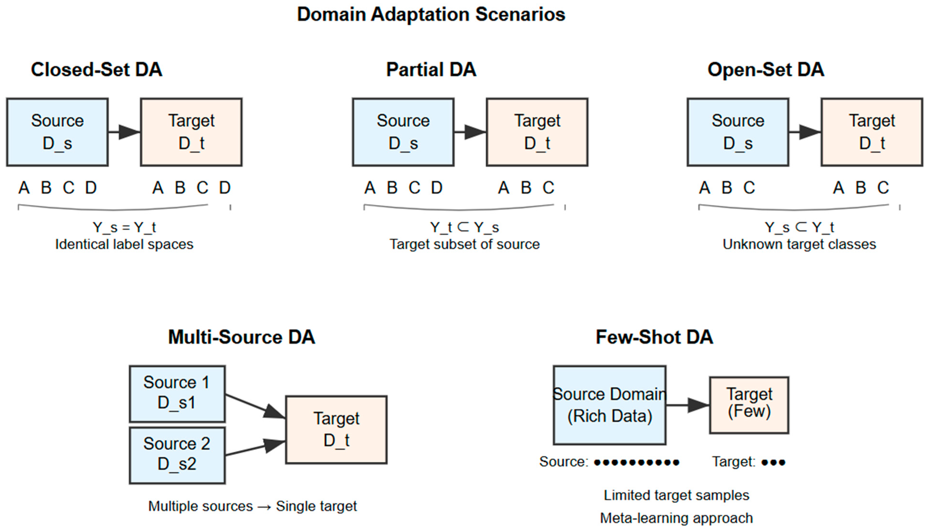
Yet moving trained models across people remains difficult: inter-subject variability, recording non-stationarities, and session effects induce substantial domain shifts. Due to the differences in emotional and physiological characteristics among different subjects, the EEG data distribution varies among different subjects [4]. It shows that the emotion recognition model trained with EEG data on a single subject may not achieve satisfactory results on a new subject, that is, there is a problem of model generality. In realistic deployments, the target domain may also contain emotion states absent from the source, creating an open-set scenario. In open-set domain adaptation (OSDA), the model must (i) align only the shared classes between domains and (ii) reject unknowns to avoid negative transfer. This setting is common in cross-dataset and cross-subject EEG but remains underexplored relative to closed-set transfer.

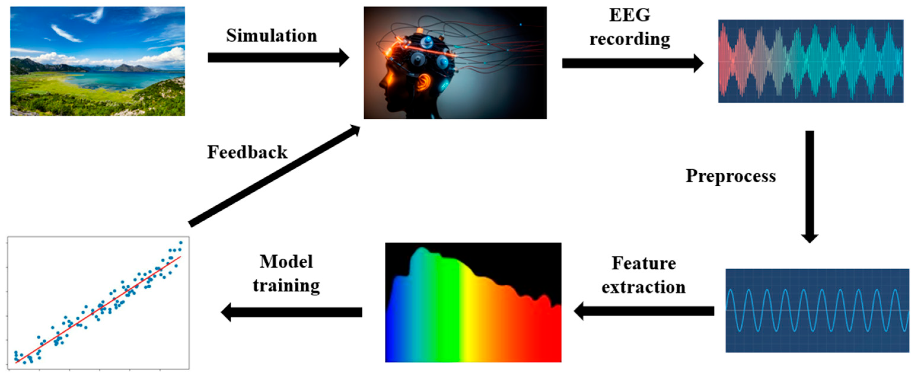
As illustrated in Figure 1, the emotional brain–computer interface (EBCI) framework typically comprises several key stages, including stimulus presentation, electroencephalogram (EEG) signal acquisition, preprocessing, feature extraction, model training, and feedback. This iterative cycle enables the systematic modeling and analysis of EEG signals to infer users’ emotional states, thereby providing a foundation for advanced human–computer interaction.

To address this, many studies have used Unsupervised Domain Adaptation (UDA) techniques [5]. These methods treat labeled EEG data from one subject as the source domain and unlabeled EEG data from another subject as the target domain. Then they train the model on the source domain to transfer it to the target domain.

Existing EEG approaches typically fall into three groups. Subject-dependent models achieve high accuracy but require labeled data per user and do not transfer. Closed-set domain adaptation reduces distribution shift but implicitly forces all target samples to match source classes, which misaligns truly novel target states. Finally, recent graph-based or temporal models improve representation quality but often rely on static inter-channel topologies and lack mechanisms to (a) encode neurocognitive priors that aid generalization, (b) capture evolving temporal salience, and (c) separate known vs. unknown target samples during adaptation. Moreover, evaluations frequently report overall accuracy alone, obscuring the trade-off between known-class performance and unknown-class rejection.

Although these existing methods effectively reduce the distribution differences in EEG data, they still have limitations. Because they usually assume that different subjects share the same label space, but the actual scene may encounter a different label space, especially when the emotional label space of the target domain is more than that of the source domain, that is, the scene of an open-set. In open-set EEG emotion recognition, not only do we need to address the distribution differences between subjects, but we also need to tackle the separation of known and unknown emotional classes due to different label spaces [6].

We address these gaps with C2FDA-G, a cognition-prior spatio-temporal graph framework integrated with a coarse-to-fine open-set adaptation pipeline. This approach leads to the proposal of the C2FDA framework for EEG emotion recognition, which is designed to overcome the identified challenges in open-set domain adaptation. On the representation side, we construct a dynamic brain graph with graph convolution to learn data-driven channel affinities, combine it with temporal self-attention to weight informative segments, and fuse the streams via hierarchical cross-attention fusion (H-CAF). In parallel, we inject a cognition-prior branch from functional connectivity (e.g., PLV), then fuse prior- and data-driven embeddings to obtain discriminative, interpretable features stable across subjects.

Initially, the Coarse-to-Fine processing module performs coarse classification on the extracted EEG feature information, sorts all target domain samples based on the similarity of each target domain sample, and selects high and low probability score samples for fine classification, thus achieving the separation of known and unknown classes in the target domain. On the adaptation side, a bank of one-vs-class coarse heads ranks target samples by known-class plausibility; a fine unknown detector assigns an unknown probability w(x). We then perform instance-weighted adversarial alignment that emphasizes likely known target samples in the shared label space using a |Cs| + 1 classifier (with an explicit unknown class). A lightweight curriculum penalizes early high-confidence misclassifications, improving the stability of unknown rejection. Then, the Domain Adversarial module maps samples from the source and target domains to a shared label space, achieving alignment of the sample space. Finally, we input the EEG signal data processed by the two modules into the classifier to complete the EEG emotion recognition task.

In summary, our research makes the following contributions:

(1) We propose a Coarse-to-Fine processing module that can separate known and unknown emotional classes. This module solves the problem of negative transfer caused by the misalignment of unknown classes in the target domain with known classes in the source domain effectively.

(2) We propose a Domain Adversarial module that maps samples from the source and target domains to a shared label space for alignment of the EEG samples. This module effectively addresses the label space alignment problem in open-set EEG emotion recognition.

(3) Through extensive transfer experiments on three datasets, our experimental results demonstrate the reliability of the C2FDA method in open-set EEG emotion recognition.

As the field of semantic communication in 6G networks continues to develop, the focus is on transmitting task-relevant meaning rather than raw data. EEG-based emotion recognition is inherently semantic, as it extracts emotionally meaningful states from complex signals. The open-set scenario naturally aligns with semantic communication principles, where the system must determine whether incoming data belongs to the known semantic space or represents novel, unrecognized states. Our C2FDA framework addresses this by filtering semantically relevant emotional information and rejecting unknown samples, thus enhancing semantic efficiency and robustness in next-generation network applications. However, it is important to note that the connection to 6G semantic communication is conceptual, and this paper focuses primarily on the development and evaluation of the C2FDA framework for EEG emotion recognition.

2. Related Work

EEG-based emotion recognition faces significant challenges in cross-subject and cross-dataset transfer due to distribution shifts between source and target domains. Based on the relationship between label spaces, existing domain adaptation approaches can be categorized into five main paradigms, as illustrated in Figure 2.

2.1. Closed-Set Domain Adaptation

Closed-Set Domain Adaptation (CSDA) assumes identical label spaces between source and target domains, focusing on reducing distribution discrepancies. These methods primarily fall into metric-based approaches and adversarial training strategies [7,8,9]. Metric-based methods transform features to minimize domain distances under specific metrics. Xu et al. [10] proposed a dynamic adversarial domain adaptive network based on the multi-kernel maximum mean discrepancy (MK_DAAN), which addresses domain adaptation by adding an adaptive layer to further align the feature distribution between source and target domains. Multi-kernel maximum mean discrepancy is adopted in the adaptive distance measurement. This dual feature alignment approach, combining the adaptive layer with adversarial learning, improves classification performance in breast ultrasound image classification. Yi et al. [11] introduced the ATPL framework, which mutually promotes adversarial training and pseudo-labeling for unsupervised domain adaptation. ATPL produces high-confidence pseudo-labels through adversarial training, and uses these pseudo-labels to improve the adversarial training process by generating adversarial data to fill the domain gap, thereby ensuring both feature transferability and discriminability. DANN (Domain-Adversarial Neural Networks), proposed by Ganin et al., uses adversarial training with a gradient reversal layer to learn domain-invariant features, improving performance in tasks like image classification and sentiment analysis. It outperforms traditional methods by aligning feature distributions between source and target domains without requiring labeled target data [12]. MMD (Maximum Mean Discrepancy), proposed by Gretton et al., is a kernel-based method for comparing distributions by measuring the difference between their means in a Reproducing Kernel Hilbert Space (RKHS). It effectively minimizes domain shift in closed-set domain adaptation and has been widely used in tasks involving high-dimensional feature spaces, such as bioinformatics and graph data [13]. CORAL (CORrelation ALignment), introduced by Sun et al., aligns the second-order statistics (covariance) between source and target domains to reduce domain shift in unsupervised domain adaptation. It has proven effective in object recognition tasks, outperforming methods like LDA on benchmark datasets such as Office-Caltech10 [14]. CDAN (Conditional Domain Adversarial Network), introduced by Long et al., enhances adversarial domain adaptation by conditioning the domain discriminator on both feature representations and classifier predictions. This approach improves alignment across domains and has shown superior performance on benchmark datasets [15].

2.2. Partial Domain Adaptation

Partial Domain Adaptation (PDA) addresses scenarios where the target label space constitutes a subset of the source domain. Here, the source contains emotional categories absent in the target, though these remain known categories. Feng et al. [16] proposed Progressive Optimization For Partial Domain Adaptation (EBB), which selects anchors by analyzing base model features and estimates category gaps using anchor classification distributions. This approach minimizes shared class errors while correcting blind alignment mistakes. Zhang et al. [17] developed Weighted and Center-aware Adaptation Learning (WCAL), distinguishing unknown source classes through weighted adversarial learning and addressing negative transfer via cross-domain discriminators. While these methods handle partial scenarios effectively, they still assume no target-specific unknown classes, differing fundamentally from open-set challenges.

2.3. Open-Set Domain Adaptation

Open-Set Domain Adaptation (OSDA) represents the most challenging setting, where target domains contain both source-known classes and completely novel categories. OSDA methods must simultaneously align shared classes while detecting unknown samples to prevent negative transfer. Panareda Busto and Gall introduced Open Set Domain Adaptation, which addresses domain shift by jointly solving an assignment problem to match target instances with source categories of interest. Their method outperforms state-of-the-art techniques, effectively handling both closed and open-set scenarios where the source and target domains may contain different class labels [18]. Ji et al. [19] proposed an open-set domain adaptation model based on subdomain alignment, using variable weights for discriminative training and aligning category subspaces between source and target domains. Experiments show that this approach significantly improves open-set domain adaptation classification accuracy. Tang et al. [20] proposed a novel open-set domain adaptation method combining latent structure discovery and kernelized classifier learning to improve class separation. Experiments on five image datasets demonstrate its superiority over state-of-the-art methods. Open-set recognition has also been explored in other domains such as malware traffic analysis [21], radio frequency fingerprint identification [22], specific emitter recognition [23], and device recognition in satellite-terrestrial-integrated IoT [24], demonstrating the broad applicability of open-set methodologies. OSBP (Open Set Back-Propagation), proposed by Saito et al., uses adversarial training to align known target samples with the source domain while rejecting unknown target samples. It outperforms traditional domain adaptation methods in open-set scenarios, improving performance in domain transfer tasks [25,26]. MAOSDAN (Multi-Adversarial Open-Set Domain Adaptation Network), proposed by Zheng et al., addresses open-set domain adaptation in remote sensing by combining attention-aware OSBP, adversarial learning, and adaptive entropy suppression to distinguish known and unknown samples [27].

2.4. Graph-Based EEG Representation Learning

EEG’s inherent spatial organization motivates graph neural network applications, treating electrodes as nodes with functional connections as edges. Static graph methods based on physical distances or fixed connectivity capture spatial topology but cannot adapt to dynamic brain connectivity changes. Liu et al. [28] compared DCCA and BDAE for multimodal emotion recognition, extending DCCA with weighted sum and attention-based fusion methods. DCCA achieved state-of-the-art performance and demonstrated greater robustness against noise across multiple datasets, including SEED-V and DREAMER. Song [29] proposed a novel Dynamical Graph Convolutional Neural Network (DGCNN) for EEG emotion recognition, dynamically learning the intrinsic relationships between EEG channels for more discriminative feature extraction. Extensive experiments on the SEED and DREAMER datasets show that DGCNN outperforms state-of-the-art methods, achieving high recognition accuracy in both subject-dependent and subject-independent settings. However, most graph-based EEG works address closed-set classification without explicit open-set label mismatch handling. Finally, we input the EEG signal data processed by the two modules into the classifier to complete the EEG emotion recognition task. Recent studies have also explored the use of attention mechanisms and hybrid deep neural networks for improving EEG-based emotion recognition performance [30,31].

2.5. Cognitive Priors in Graph Learning

Neuroscience research indicates functional connectivity patterns, measured through phase-locking value (PLV), encode task-relevant brain network structures. Incorporating such cognition-inspired priors improves interpretability and cross-domain stability. Recent cognitive-prior GNN frameworks fuse prior graphs with data-driven graphs, yielding noise-robust representations stable across subjects [32]. Li et al. [33] proposed a graph learning system for EEG-based emotion recognition, utilizing a cognition-inspired functional graph branch and a fused attention mechanism to automatically learn emotion-related cognitive patterns. The BF-GCN model outperforms state-of-the-art methods, achieving high recognition accuracy in both subject-dependent and subject-independent experiments on the SEED and SEED-IV datasets. Wang et al. [34] proposed a simply ameliorated CNN (SACNN) for cross-subject emotion recognition using raw EEG data to address low accuracy issues in driver emotion detection. The SACNN model achieved 88.16% accuracy with cross-subject data and 91.85% accuracy using data from the top 10 EEG channels, outperforming deeper models and highlighting its potential for smart city applications. Furthermore, cross-subject emotion recognition remains challenging due to inter-subject variability, prompting the development of methods that leverage raw multi-channel EEG data without extensive preprocessing [35]. Machine learning approaches continue to evolve, with comparative studies highlighting the effectiveness of various algorithms in handling EEG-based emotion recognition tasks [36].

Our proposed C2FDA addresses these gaps by combining cognition-prior spatio-temporal graph encoding with coarse-to-fine open-set adaptation. This unified framework leverages neuroscience knowledge while providing robust mechanisms for known-unknown separation and selective domain alignment, advancing the state-of-the-art in open-set EEG emotion recognition. C2FDA integrates a complex cognition-prior spatio-temporal graph encoder as part of its feature extraction mechanism, which ensures robust cross-domain generalization, particularly for open-set scenarios.

2.6. Semantic Communication and Next-Generation Networks

Semantic communication represents a paradigm shift from bit-level accuracy to goal-oriented information exchange, focusing on the meaning and effectiveness of transmitted data. In next-generation networks (6G), semantic communication aims to reduce redundancy by transmitting only task-relevant information, thereby improving bandwidth efficiency and latency. Emotion recognition from EEG signals is a semantically rich task, as emotions represent high-level cognitive states. Recent works have explored semantic source coding, task-oriented communication, and semantic-aware resource allocation for IoT and edge devices [37,38,39]. Our C2FDA framework aligns with this trend by selectively adapting only known emotional classes and rejecting unknowns, effectively reducing semantic redundancy and improving communication efficiency in distributed EEG-based emotion recognition systems.

3. Methodology

We begin by establishing the notation used throughout this work. Let ${\mathrm{D}}_{\mathrm{s}}={\left({\mathrm{x}}_{\mathrm{i}}^{\mathrm{s}},{\mathrm{y}}_{\mathrm{i}}^{\mathrm{s}}\right)}_{\mathrm{i}=1}^{{\mathrm{n}}_{\mathrm{s}}}$ denote the source domain with ${\mathrm{n}}_{\mathrm{s}}$ labeled samples, and ${\mathrm{D}}_{\mathrm{t}}={{\mathrm{x}}_{\mathrm{j}}^{\mathrm{t}}}_{\mathrm{j}=1}^{{\mathrm{n}}_{\mathrm{t}}}$ represent the target domain with ${\mathrm{n}}_{\mathrm{t}}$ unlabeled samples. The label space relationship follows ${\mathrm{C}}_{\mathrm{s}}\subset {\mathrm{C}}_{\mathrm{t}}={\mathrm{C}}_{\mathrm{s}}\cup \mathrm{U}$, where U denotes the set of unknown classes present only in the target domain. Our framework employs a feature extractor ${\mathrm{f}}_{\mathsf{\theta }}:\mathrm{x}\mapsto \mathrm{z}\in {\mathrm{R}}^{\mathrm{d}}$ that maps inputs to d-dimensional representations. The coarse-stage processing utilizes a bank of one-vs-rest classifiers ${{\mathrm{h}}_{\mathrm{k}}}_{\mathrm{k}\in {\mathrm{C}}_{\mathrm{s}}}$, each producing class-specific probabilities ${\mathrm{p}}_{\mathrm{k}}\left(\mathrm{x}\right)=\mathsf{\sigma }\left({\mathrm{h}}_{\mathrm{k}}\left({\mathrm{f}}_{\mathsf{\theta }}\left(\mathrm{x}\right)\right)\right)$. The fine-stage unknown detector ${\mathrm{u}}_{\mathsf{\phi }}:\mathrm{z}\mapsto \mathrm{w}\left(\mathrm{x}\right)\in \left[\mathrm{0,1}\right]$ estimates the probability that a sample belongs to an unknown class. Finally, an open-set classifier ${\mathrm{H}}_{\mathrm{y}}:\mathrm{z}\mapsto \mathrm{ŷ}\in 1,\dots ,\left|C_s\right|,unk$ performs $\left|{\mathrm{C}}_{\mathrm{s}}\right|+1$ classification, while a domain discriminator ${\mathrm{D}}_{\mathsf{\psi }}:\mathrm{z}\mapsto \mathrm{0,1}$ distinguishes between source and target domains. Having established the notation, we now proceed to detail the architecture and training procedure of our proposed C2FDA framework.

The method addresses two fundamental challenges in open-set domain adaptation: (1) distinguishing between known and unknown classes in the target domain, and (2) aligning only the shared classes while avoiding negative transfer from unknown samples. For the sake of illustration, we give some definitions of symbols. In the open-set EEG emotion recognition task, we have a source domain Ds containing ns labeled samples, denoted as $D_s={\left\{\left(x_i^s,y_i^s\right)\right\}}_{i=1}^{n_s}$, and a target domain Dt containing nt unlabeled samples, denoted as $D_t={\left\{\left(x_j^T\right)\right\}}_{j=1}^{n_t}$. Here, the label space size of the source domain is Cs. It is worth noting that the label space of the source domain is a subset of the label space of the target domain: $C_s\subset C_t$ The additional label space contained in the target domain is defined as the unknown class label space $C_{t\setminus s}$.

The source domain and the target domain come from different probability distributions $p,q$, respectively. In domain adaptation, our probability distribution is also different: $p\ne q.$ In open-set domain adaptation, our probability distributions are even more different: $p\ne q_{C_s}$, where $q_{C_s}$ represents the distribution of target domain data in the shared label space. In summary, we can define the open-set EEG emotion recognition task as follows: $O=1-{\displaystyle \frac{\left|C_s\right|}{\left|C_t\right|}}$. It is important to note that the label space of our source domain is a subset of the label space of the target domain.

3.1. C2FDA Model

Cognition-Prior Spatio-Temporal Graph Encoder—This component extracts discriminative and interpretable EEG features by combining dynamic graph convolution (DGC), temporal self-attention (TSAR), and hierarchical cross-attention fusion (H-CAF) along with a functional connectivity prior represented by the PLV graph.

Coarse-to-Fine Selector—This component ranks target samples based on their plausibility of belonging to the shared classes and then refines the decisions using a binary classification (“unknown vs. known”) fine head.

Instance-Weighted Domain Adversarial Alignment—This component aligns only the target samples likely to belong to the known classes to the source domain using a gradient reversal layer (GRL), while suppressing the alignment of unknown samples.

Open-Set Classifier—This component predicts over |Cs| + 1 classes, where the additional class explicitly represents the “unknown” category.

To address the aforementioned two issues, we innovatively propose A Coarse-to-Fine Open-set Domain Adaptation framework for EEG emotion recognition (C2FDA). The method framework of C2FDA is illustrated in Figure 2. This method mainly consists of two modules: the Coarse-to-Fine processing module and the Domain Adversarial module. The Coarse-to-Fine processing module transforms the extracted EEG feature information from coarse-grained features to fine-grained features; in other words, its purpose is to separate known classes from unknown classes. The function of the Domain Adversarial module is to map samples from the source domain and target domain to a common label space, achieving sample space alignment. In Figure 2, $H_f$ represents the feature extractor of EEG signals, $H_{\mathrm{coarse} }$ and $H_{\mathrm{fine} }$ represent the coarse classifier and fine classifier, respectively, $H_d$ is the domain discriminator, which is also our Domain Adversarial module, and $H_y$ is our final EEG data classifier. C2FDA-G is a variant of C2FDA that incorporates a cognition-prior spatio-temporal graph encoder into the feature extraction process, enhancing the model by explicitly integrating neurocognitive priors from EEG signals. Both models share the same core feature extraction approach, but C2FDA-G benefits from the added graph encoder for richer spatio-temporal dependencies.

3.2. Cognition-Prior Spatio-Temporal Graph Encoder

(a) Graph Construction We represent each EEG trial as a multi-channel DE feature map over $B$ frequency bands. Each band yields a graph $G=\left(V,E,A\right)$, where $V$ are channels, $E$ edges, and $A$ the adjacency matrix.

To capture both neurophysiological priors and adaptive patterns, we construct a hybrid graph representation that combines domain knowledge with data-driven learning: Prior Graph $A_{\mathrm{prior} }$—computed from PLV between channels over source data, encoding stable cognitive connectivity patterns.

Data-Driven Graph $A_{\mathrm{data} }$—learned via attention-based affinity estimation that adapts to each sample.

$$\begin{array}{c}A=\alpha A_{p}rior+\left(1-\alpha \right)A_{d}ata,\end{array}$$

(1)

$$where A_{d}ata=softmax\left(Q{K}^T/\sqrt{d}\right)$$

The parameter α balances the contribution of cognitive priors (when α is large) versus adaptive learning (when α is small), allowing the model to leverage neuroscience knowledge while adapting to task-specific patterns.

We blend the two to form the adjacency for convolution:

$$\begin{array}{c}\hat{A}=\left(1-\lambda \right)A_{\mathrm{prior} }+\lambda A_{\mathrm{data} },\lambda \in \left[\mathrm{0,1}\right].\end{array}$$

(2)

(b) Spatial Encoding with DGC We apply graph convolutional layers over $\hat{A}$ to capture spatial dependencies:

$$\begin{array}{c}{H}^{\left(l+1\right)}=\sigma \left({\hat{D}}^{-1/2}\hat{A}{\hat{D}}^{-1/2}{H}^{\left(l\right)}{W}^{\left(l\right)}\right)\end{array}$$

(3)

where $\hat{D}$ is the degree matrix, $W^{\left(l\right)}$ are learnable weights, and $\sigma$ is an activation function.

$$\begin{array}{c}{Z}^{\left(l+1\right)}=\sigma \left({\tilde{D}}^{\left(-1/2\right)}{\widetilde{\mathrm{Ã}D}}^{\left(-1/2\right)}{Z}^{\left(l\right)}{W}^{\left(l\right)}\right),Ã=A+I\end{array}$$

(4)

(c) Temporal Self-Attention (TSAR) For each channel representation, TSAR assigns attention weights across time steps:

$$\begin{array}{c}{\alpha }_t={\displaystyle \frac{\exp \left(q_t^{\mathrm{\top }}{k}_t\right)}{\sum _{t^{\text{'}}} \exp \left(q_{t^{\text{'}}}^{\mathrm{\top }}{k}_{t^{\text{'}}}\right)}},\end{array}$$

(5)

where $q_t,k_t$ are learned projections. This emphasizes temporally salient EEG segments.

$$\begin{array}{c}Attn\left(Q,K,V\right)=softmax\left(Q{K}^T/\sqrt{d}\right)V,z=Pool\left(Attn\left(·\right)\right)\end{array}$$

(6)

(d) Hierarchical Cross-Attention Fusion (H-CAF) Spatial and temporal streams are fused using cross-attention to produce the final embedding $\mathit{f}$ for each trial.

3.3. Hyperparameter Tuning for α and λ

In this section, we explain the selection of the hyperparameters α and λ, which are essential for the performance of the C2FDA framework. The parameter α controls the balance between cognitive priors and adaptive learning, while λ adjusts the weight of the entropy loss in the domain adversarial module. The two parameters determine how the model blends prior knowledge and data-driven learning, ensuring effective separation between known and unknown emotional classes.

To blend the cognitive prior graph ($A_{prior}$) and the data-driven graph ($A_{data}$), we use the equation:

$$A=\alpha A_{prior}+(1-\alpha )A_{data},\alpha \in \left[\mathrm{0,1}\right]$$

(7)

The parameter α was tested within the range [0.1, 1.0], where larger values favor prior knowledge and smaller values prioritize adaptive learning. Similarly, λ controls the entropy loss contribution and was varied within [0, 1], with higher values placing more emphasis on rejecting unknown classes. The adjusted adjacency matrix is given by:

$$\widehat{A}=(1-\lambda )A_{prior}+\lambda A_{data},\lambda \in \left[\mathrm{0,1}\right]$$

(8)

We used k-fold cross-validation to select the optimal values for both α and λ, evaluating performance based on recognition accuracy for known classes and the ability to detect unknown emotional states. The impact of these hyperparameters is significant. Larger α values improve known-class recognition but reduce flexibility in detecting unknown emotional states, while smaller values enhance detection of novel classes. For λ, higher values strengthen unknown class rejection but may overfit known classes, while lower values improve detection of unknowns. This tuning process ensures robustness and reproducibility in open-set EEG emotion recognition tasks.

3.4. The Coarse-to-Fine Processing Module

Coarse Stage: We deploy a bank of $\left|C_s\right|$ one-vs-class classifiers $\left\{h_k\right\}$ producing logits $z_k$ and probabilities $p_k=\sigma \left(z_k\right)$. For target sample $x$, define:

$$\begin{array}{c}s\left(x\right)=\underset{k\in C_s}{\mathrm{m}\mathrm{a}\mathrm{x}} p_k \end{array}$$

(9)

To distinguish known and unknown classes in the target domain, we put forward the Coarse-to-Fine processing module. We introduce a coarse classifier $H_{\mathrm{coarse}=1 }^{\left|C_s\right|}$, consisting of $\left|C_s\right|$ classifiers. The coarse classifier measures the similarity between each target domain sample and each source domain class. Each classifier is independent, with different functionalities; each classifier can only classify specific emotion classes. The loss function of the coarse classifier is defined as shown in Equation (1):

$$\begin{array}{c}{L}_s={\displaystyle \sum _{\mathrm{coarse} =1}^{\left|C_s\right|}} {\displaystyle \frac{1}{n_s}}{\displaystyle \sum _{i=1}^{n_s}} L_{bce}\left(H_{\mathrm{coarse} }\left(H_f\left(x_i^s\right)\right),I\left(y_i^s,\mathrm{c}\mathrm{o}\mathrm{a}\mathrm{r}\mathrm{s}\mathrm{e}\right)\right)\end{array}$$

(10)

In Equation (10), $L_{bce}$ represents the cross-entropy loss of the coarse classifier. When $y_i^s=$ coarse, $I\left(y_i^s, \mathrm{coarse} \right)$ = 1; otherwise, $I\left(y_i^s, \mathrm{coarse} \right)$ = 0. Each $H_{\mathrm{coarse} }$ returns the probability score $P_{\mathrm{coarse} }$ of each target domain sample being classified as the known class coarse. Thus, $P_{\mathrm{coarse} }$ can be used to measure the similarity between samples in the target domain and the known class. A higher probability score indicates a higher likelihood of the sample belonging to class coarse. Empirically, known class samples in the target domain tend to have higher probability scores compared to unknown class samples. Therefore, we can use the maximum probability score of each sample, p1, p2, …, p$\left|C_s\right|$, to represent the similarity between each target domain sample $x_j^t$ and the source domain, as shown in Equation (2):

$$\begin{array}{c}{s}_j=\underset{c\in C_s}{\mathrm{m}\mathrm{a}\mathrm{x}} H_{\mathrm{coarse} }\left(H_f\left(x_j^t\right)\right)\end{array}$$

(11)

To avoid manual hyperparameter tuning and ensure robustness across different degrees of openness, we introduce an adaptive thresholding mechanism based on quantile statistics:

$$\begin{array}{c}{\tau }_{\left(high\right)}=E_{x\in Q_{\mathrm{\top }}q}\left[s\left(x\right)\right],{\tau }_{\left(low\right)}=E_{x\in Q_{\perp }q}\left[s\left(x\right)\right]\end{array}$$

(12)

$$T_K=x:s\left(x\right)\ge {\tau }_{\left(high\right)},T_U=x:s\left(x\right)\le {\tau }_{\left(low\right)}$$

(13)

Figure 3 Coarse-to-fine sample separation via adaptive threshold selection. Target domain samples are stratified into three regions based on similarity scores: high-confidence known sample region (green) for domain alignment; ambiguous sample region (gray) excluded from training; and high-confidence unknown sample region (red) for novel class detection. The high and low adaptive thresholds are automatically determined without hyperparameter tuning. This approach is conceptually similar to the Separate to Adapt (STA) method, which employs a coarse-to-fine separation mechanism to progressively distinguish between known and unknown classes based on sample similarity. In STA, sample importance is adaptively weighted during feature distribution alignment, and unknown target samples are excluded from the alignment process to prevent negative transfer. While STA addresses domain adaptation across varying levels of openness, this work utilizes adaptive threshold selection to specifically tackle the challenges of open-set EEG emotion recognition without the need for manual hyperparameter tuning.

This partitioning strategy creates three distinct regions: high-confidence known samples (${\mathrm{T}}_{\mathrm{K}}$), high-confidence unknown samples (${\mathrm{T}}_{\mathrm{U}}$), and an ambiguous region $T_A=D_t\mathrm{ }\left(T_K\cup T_U\right)$ that is excluded from alignment to prevent negative transfer.

After employing such a measurement method, known class samples in the target domain will indeed exhibit high similarity with the source domain. Similarly, samples of unknown classes in the target domain will show low similarity with the source domain.

Therefore, based on the magnitude of similarity for each target domain sample, we can sort all target domain samples and select those with particularly high or low probability scores to train the next-stage fine classifier $H_{\mathrm{fine} }$. Although this selection method may seem simplistic, the chosen samples exhibit high confidence and similarity. Additionally, since we no longer need to manually select hyperparameters or use optimization tools, this approach is robust to varying degrees of openness.

To further refine sample selection, we categorize samples into three groups based on the magnitude of similarity probability scores: highest probability scores, moderate probability scores, and lowest probability scores. Then, we use the average of the highest probability scores, denoted as $s_{\mathrm{h} }$, as the upper limit for known class samples in the target domain. Thus, when a sample’s similarity probability score satisfies $s_{\mathrm{j} }$ ≥ $s_{\mathrm{h} }$, we classify it as a known class. Similarly, we use the average of the lowest probability scores, denoted as $s_{\mathrm{l} }$, as the lower limit for unknown class samples in the target domain. Hence, when a sample’s similarity probability score satisfies $s_{\mathrm{j} }$≤ $s_{\mathrm{l} }$, we classify it as an unknown class.

Fine Stage: From the extreme quantiles (top $q_{hi}\%$, bottom $q_{lo}\%$ of $s\left(x\right)$), a binary fine classifier $h_{\mathrm{fine} }$ is trained to predict $w\left(x\right)$, the probability that $x$ is unknown. While the coarse stage provides initial separation, the fine-stage binary classifier performs precise unknown detection by learning from the high-confidence samples identified in the coarse stage.

As illustrated in Figure 4, the C2FDA framework adopts a hierarchical processing strategy. First, a graph-based feature extractor (which incorporates the cognition-prior spatio-temporal graph encoder in C2FDA-G) processes EEG signals from both the source and target domains. This feature extraction approach combines a simpler feature extractor ($H_f$) in C2FDA and a more complex graph encoder in C2FDA-G, both of which share the same fundamental task of extracting relevant features from the EEG signals. Then, the coarse-to-fine separation module performs progressive filtering on the target samples. Specifically, the coarse separation layer ranks the samples based on their similarity to known categories, while the fine separation layer conducts binary classification to distinguish between known and unknown samples. Finally, the domain adversarial module aligns distributions only for the samples that are likely to belong to known categories, thereby avoiding negative transfer caused by unknown samples. This allows the final classifier to achieve open-set emotion recognition with unknown category detection.

Once the coarse classifier $H_{\mathrm{coarse} }$ selects high probability known class samples and low probability unknown class samples, denoted as $X^{\text{'}}$, we can further feed these selected samples into the next-stage fine classifier $H_{\mathrm{fine} }$, to separate known and unknown class samples in the target domain. We label the samples that have been separated from the target domain, denoted as $x_j$∈$X^{\text{'}}$, as $d_j$. Known class samples are labeled as $d_j$ = 0, while unknown class samples are labeled as $d_j$ = 1. The loss function of the fine classifier $H_{\mathrm{fine} }$ is shown in Equation (3):

$$\begin{array}{c}w\left(x\right)=\sigma \left(u_{\phi }\left(f_{\theta }\left(x\right)\right)\right)\end{array}$$

(14)

$$\begin{array}{c}{L}_{f}ine=\left(1/\left|S\right|\right){\displaystyle \sum _{x\in S}}BCE\left(y_{u}nk\left(x\right),w\left(x\right)\right)\end{array}$$

(15)

The unknown probability w(x) serves as an instance-level confidence measure, enabling selective alignment where only samples with low w(x) values (likely known) participate in domain adversarial training. Through the Coarse-to-Fine processing module, we can separate EEG signal samples of known and unknown classes in the target domain.

Curriculum Learning: Inspired by step-penalty reinforcement learning, we weight early confident mistakes more heavily in the first K epochs:

$$\begin{array}{c}{\alpha }_e={\alpha }_0+\left(1-{\alpha }_0\right){\displaystyle \frac{e}{K}}.\end{array}$$

(16)

Through the Coarse-to-Fine processing module, we can separate EEG signal samples of known and unknown classes in the target domain.

From a semantic communication perspective, the coarse-to-fine mechanism acts as a semantic filtering process: it transmits only emotionally relevant information (known classes) while suppressing irrelevant or unknown samples. This aligns with the goal of semantic communication in 6G systems, where only semantically valid data is prioritized for transmission, thereby reducing bandwidth overhead and improving task efficiency.

3.5. The Domain Adversarial Module

Traditional domain adaptation aligns all target samples with the source distribution, leading to negative transfer when unknown classes are present. Our instance-weighted alignment strategy addresses this by selectively emphasizing likely known samples.

In this section, we first present the classification error function for the source domain, as shown in Equation (4):

$$\begin{array}{c}{L}_{\mathrm{c}\mathrm{l}\mathrm{s}}^s={\displaystyle \frac{1}{n_s}}{\displaystyle \sum _{x_i\in D_s}} L_y\left(H_y^{\left(1:\left|C_s\right|\right)}\left(H_f\left(x_i\right)\right),y_i\right)\end{array}$$

(17)

where Ly represents the cross-entropy loss function, and Hy represents an extended classifier with |Cs| + 1 classes, where |Cs| + 1 includes |Cs| known emotions from the source domain and 1 unknown emotion from the target domain. Therefore, $H_y^{\left(1:\left|C_s\right|\right)}$ returns the probability of each sample corresponding to the |Cs| known emotions.

Next, we focus on aligning the features of samples from the source and target domains. In this step, we map the features from both domains to a shared label space, denoted as Cs. Instead of directly inputting the output of $H_{\mathrm{fine} }$ into discriminators for known and unknown classes, we append a softmax layer to the output of $H_{\mathrm{fine} }$, which serves as the input to the discriminators. This softmax layer generates soft instance-level weights, denoted as $w_j=H_b\left(H_f\left(x_j\right)\right)$, where higher values of $w_j$ indicate a higher probability of the sample belonging to the unknown class. Hence, we can utilize $w_j$ to define the weighted loss for Domain Adversarial adaptation of feature distributions in the shared label space Cs, as shown in Equation (5):

$$\begin{array}{c}\begin{array}{ll}{L}_d=& {\displaystyle \frac{1}{n_s}}{\displaystyle \sum _{x_i\in D_s}} L_{bce}\left(H_d\left(H_f\left(x_i\right)\right),d_i\right)\\ & +{\displaystyle \frac{1}{\sum _{x_j\in D_t} \left(1-w_j\right)}}{\displaystyle \sum _{x_j\in D_t}} \left(1-w_j\right)L_{bce}\left(H_d\left(H_f\left(x_j\right)\right),d_j\right)\end{array}\end{array}$$

(18)

In addition, we also need to select samples of unknown classes from the target domain to train the feature extractor Hf. Based on the soft instance-level weights $w_j$, we can measure the separation between known and unknown classes. We define the weighted loss for distinguishing unknown classes as shown in Equation (6):

$$\begin{array}{c}{L}_{\mathrm{c}\mathrm{l}\mathrm{s}}^t={\displaystyle \frac{1}{\left|C_s\right|}}{\displaystyle \frac{1}{\sum _{x_j\in D_t} w_j}}{\displaystyle \sum _{x_j\in D_t}} w_j{L}_y\left(H_y^{\left(\left|C_s\right|+1\right)}\left(H_f\left(x_j\right)\right),l_{uk}\right)\end{array}$$

(19)

where $l_{uk}$ represents the unknown emotion class. Through training, we assign all target samples with larger weights $w_j$ to the unknown emotion class. Similarly, $H_y^{\left(\left|C_s\right|+1\right)}\left(H_f\right)$ represents the probability that classifier Hy assigns target samples to the unknown class.

We also enhance the decision boundary between domains by computing the loss for minimizing the entropy of known classes in the target domain, denoted as Le. This is achieved by enhancing weights with the following formula, as shown in Equation (7):

$$\begin{array}{c}{L}_e={\displaystyle \frac{1}{\sum _{x_j\in D_t} \left(1-w_j\right)}}{\displaystyle \sum _{x_j\in D_t}} \left(1-w_j\right)E\left(H_y^{\left(1:\left|C_s\right|\right)}\left(H_f\left(x_j\right)\right)\right)\end{array}$$

(20)

In Equation (7), E represents the entropy loss, specifically expressed as $E\left(p\right)=-\sum _k p_k\mathrm{l}\mathrm{o}\mathrm{g}{p}_k.$ It is important to note that our goal is to minimize the entropy of target samples predicted as known emotion class. Therefore, we use $w_j$ as the instance-level weight parameter for entropy minimization.

The adversarial alignment in C2FDA ensures semantic consistency across domains, akin to semantic fidelity in 6G-oriented communication systems. By weighting known samples more heavily, the model mimics a semantic-aware transmission protocol that prioritizes meaningful emotional states over noisy or unknown inputs.

3.6. Open-Set Classification and Loss Functions

Beyond global domain alignment, we introduce prototype-based fine-grained alignment to enhance intra-class consistency between source and target domains:

$${\mu }_k=\left(1/\left|S_k\right|\right){\displaystyle \sum _{\left(x,y\right)\in D_s,y=k}}{f}_{\theta }\left(x\right)$$

(21)

$$\begin{array}{c}{L}_{\left(proto\right)}={\displaystyle \sum _{k\in C_s}}{E}_{{\widehat{x\in T}}_K\left(k\right)}{\left|\left|f_{\theta }\left(x\right)-{\mu }_k\right|\right|}_2^2\end{array}$$

(22)

To stabilize the training process and prevent early convergence to suboptimal solutions, we employ a curriculum learning strategy that penalizes confident misclassifications more heavily in early training stages:

$$\begin{array}{c}{L}_{\left(curr\right)}=\left(1/\left|D_t\right|\right){\displaystyle \sum _{x\in D_t}}\gamma max\left(0,T_0-e\right)\\ ·\left[1\left(\mathrm{ŷ}\ne unk\right)·w\left(x\right)\right]\end{array}$$

(23)

where e is the current epoch, $T_0$ is the transition epoch, and γ ∈ (0,1).

Our final objective function integrates all components through a carefully designed multi-term loss that balances source supervision, sample separation, domain alignment, and regularization.

The open-set classifier $H_y$ outputs $\left|C_s\right|+1$ logits, with the last logit representing “unknown.” We optimize the total loss:

$$\begin{array}{c}L=L_{src}+{\lambda }_{co}{L}_{coarse}+{\lambda }_{fi}{L}_{fine}+{\lambda }_{adv}{L}_{adv}+{\lambda }_{pr}{L}_{proto}\\ +{\lambda }_{unk}{L}_{unk}+{\lambda }_{ent}{L}_{ent}+{\lambda }_{cur}{L}_{curr}\end{array}$$

(24)

Each loss term addresses a specific aspect of the open-set domain adaptation problem: $L_{src}$ ensures source discriminability, $L_{coarse}$ and $L_{fine}$ enable known/unknown separation, $L_{adv}$ performs selective alignment, $L_{proto}$ enhances intra-class consistency, $L_{unk}$ promotes unknown rejection, $L_{ent}$ sharpens decision boundaries, and $L_{curr}$ provides training stability.

Where each term corresponds to supervised source classification, coarse/fine stage training, adversarial alignment, target entropy minimization, and curriculum penalty.

3.7. Objective Function

The optimization of our multi-component objective requires a progressive training strategy that alternates between sample separation and domain alignment to ensure stable convergence.

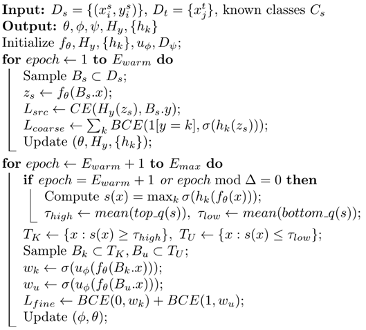
We divide the training into two progressive stages: (1) sample separation, where target data are partitioned into likely known and likely unknown subsets based on confidence scores, and (2) domain adversarial adaptation, where only the reliable known subset is aligned with the source domain distribution. By alternating between these two stages, the model gradually adapts target samples of known classes while rejecting unknown ones.

Algorithm 1 summarizes the procedure. In the first step, we train the feature extractor $f_{\theta }$ and classifier $H_y$ with source supervision, while auxiliary coarse classifiers $\left\{h_k\right\}$ provide confidence scores for sample separation. Target samples with high scores are treated as potential known data and passed to the fine classifier $u_{\varphi }$, whereas low-score samples are considered likely unknown.

This alternating optimization strategy prevents the premature alignment of unknown samples while gradually improving the separation of known and unknown classes, leading to more robust open-set domain adaptation performance.

Algorithm 1: Coarse-to-Fine Open-Set Domain Adaptation (CF-OSDA)

Step 1: First, we train the feature extractor Hf and classifier Hy on the source domain. Additionally, we utilize each class of emotion samples in the source domain to train the coarse classifiers $H_{\mathrm{coarse} }$, where coarse $=\mathrm{1,2},3,\dots ,\left|C_s\right|$. Next, we select target domain samples with high and low probability scores, similar to those in the source domain, to train the fine classifier $H_{\mathrm{fine} }$. Here, we denote the parameters of $H_f,H_y,H_{\mathrm{fine} },H_{\mathrm{coarse} }\left|\begin{array}{rr}& \left|C_s\right|\\ & c=1\end{array}\right.$ as ${\theta }_f,{\theta }_y,{\theta }_{\mathrm{fine} },{\left.{\theta }_{\mathrm{coarse} }\right|}_{\mathrm{coarse} =1}^{\left|C_s\right|}$, respectively. The optimal parameters ${\hat{\theta }}_f,{\hat{\theta }}_y,{\hat{\theta }}_{\mathrm{fine} },{\left.{\hat{\theta }}_{\mathrm{coarse} }\right|}_{\mathrm{coarse} =1}^{\left|C_s\right|}$ = 1 can be found using the following equation, as shown in Equation (8):

$$\begin{array}{c}\left({\hat{\theta }}_f,{\hat{\theta }}_y,{\hat{\theta }}_{\mathrm{fine} },{\left.{\hat{\theta }}_{\mathrm{coarse} }\right|}_{\mathrm{coarse} =1}^{\left|C_s\right|}\right)=\\ \underset{{\theta }_f,{\theta }_y,{\theta }_b,{\left.{\theta }_c\right|}_{c=1}^{\left|C_s\right|}}{\mathrm{a}\mathrm{r}\mathrm{g}\mathrm{m}\mathrm{i}\mathrm{n}}\left(L_{\mathrm{cls} }^s+L_s+L_b\right)\end{array}$$

(25)

Step 2: In this step, we primarily perform domain adversarial adaptation to align the feature distribution of known classes in the target domain with that in the source domain. Additionally, we use data from unknown classes to train Hy as additional classes. In this step, we continue training the classifiers with source samples to retain knowledge relevant to known class emotions. We denote the parameters of the domain discriminator $H_d$ as ${\theta }_d$. The optimal parameters ${\hat{\theta }}_f,{\hat{\theta }}_y,{\hat{\theta }}_{\mathrm{d} }$ can be obtained using the following two equations, as shown in Equations (9) and (10):

$$\left({\hat{\theta }}_y,{\hat{\theta }}_d\right)=\underset{{\theta }_y,{\theta }_d}{argmin}\left(L_{\mathrm{c}\mathrm{l}\mathrm{s}}^s+L_{\mathrm{c}\mathrm{l}\mathrm{s}}^t+L_d+\lambda L_e\right)$$

(26)

$${\hat{\theta }}_f=\underset{{\theta }_f}{argmin}\left(L_{\mathrm{c}\mathrm{l}\mathrm{s}}^s+L_{\mathrm{c}\mathrm{l}\mathrm{s}}^t-L_d+\lambda L_e\right)$$

(27)

where λ is a hyperparameter used to balance the entropy loss.

Through the proposed C2FDA model, we can effectively separate known and unknown class data in the target domain. Step 1 rejects unknown class emotion data to avoid interference from unknown class emotions in Step 2, where domain adversarial adaptation aligns the feature distributions of samples between the source and target domains. Since there is no manual selection of threshold hyperparameters throughout the process, the disadvantage of tuning parameters when the openness changes in real scenarios can be avoided.

In summary, the biggest problem of an open-set task is the separation of known emotions and unknown emotions. In order to solve this problem, we propose the C2FDA method. The C2FDA method uses a gradual method to find two types of samples with high scores and low scores during training. Because the prediction results of the samples with high scores will be more accurate, it is also conducive to training the classifiers of known classes, while the samples with low scores tend to be the samples of unknown classes, so we can extract these samples to train the classifiers of unknown classes. By this means, we can well separate the known emotion from the unknown emotion. At the same time, it also solves the impact of the negative migration of wrong samples.

4. Experiments and Analysis

4.1. Dataset

SEED: The SEED dataset [40,41] is a publicly available dataset for studying the relationship between emotions and EEG signals. It consists of recordings from three sessions, each containing EEG signal data from 15 subjects. In each session, subjects watched 15 video clips with varying emotional tendencies (negative, neutral, positive), as shown in Figure 5. EEG signals were recorded using a 62-channel ESI neuroimaging system at a sampling rate of 200 Hz and band-pass filtered from 0 to 75 Hz. The raw EEG signal data were processed to extract features in five frequency bands: delta (1–4 Hz), theta (4–8 Hz), alpha (8–14 Hz), beta (14–31 Hz), and gamma (31–50 Hz), producing 310-dimensional feature vectors (5 frequency bands × 62 channels).

SEED-IV: The SEED-IV dataset [42,43] contains three sessions, each with 15 subjects. In each session, subjects watched 24 video clips with different emotional tendencies (happiness, sadness, fear, neutral), as shown in Figure 6. Similar to the SEED dataset, the EEG data were processed into 310-dimensional feature vectors (5 frequency bands × 62 channels), ensuring consistency for comparison. This normalization of the EEG data allows direct comparison with SEED.

SEED-V: The SEED-V dataset [44] differs from the previous two datasets in that it includes three sessions with 16 subjects in each session. In each session, subjects watched video clips with five emotional tendencies (happiness, sadness, fear, neutral, disgust), as shown in Figure 7. Similar to the SEED and SEED-IV datasets, the EEG data were transformed into 310-dimensional feature vectors (5 frequency bands × 62 channels) to standardize the data across all datasets. This ensures consistency in the EEG data representation.

Differences Between Datasets

Table 1. Differences between the SEED, SEED-IV, and SEED-V datasets.

Item	SEED	SEED-IV	SEED-V
Emotions	Positive, Negative, Neutral	Happy, Sad, Neutral, Fearful	Happy, Sad, Disgust, Neutral, Fearful
Number of Subjects	15	15	16
Video Clips	15	24	15
Video Length	4 min	2 min	50 min
Sample Length	1 s	4 s	15–30 s
Number of Samples	≈3394	≈843	≈681

outlines the key differences among the three datasets, including the number of subjects, video clips, and emotion categories, highlighting the increasing complexity of label spaces, especially from SEED to SEED-V. The differences between the three datasets are shown in Table 1.

4.2. Implementation Details

In our experiments, we use the SEED, SEED-IV, and SEED-V datasets to validate the performance of the C2FDA method in the open-set EEG emotion recognition task. The experiments are conducted across three main transfer scenarios, which differ in the number of emotional categories:

• SEED contains 3 emotions
• SEED-IV contains 4 emotions
• SEED-V contains 5 emotions

To investigate the model’s performance further, we conduct experiments with the following transfer scenarios: “SEED → SEED-IV”, “SEED-IV → SEED-V”, and “SEED → SEED-V”. The source domain in each scenario consists of data from 15 or 16 subjects in one session, while the target domain consists of data from a single subject in one session. Each dataset has three sessions, which allows us to test the model under different conditions and obtain reliable results.

Due to the inconsistency in label spaces between the datasets—SEED having 3 emotion classes, SEED-IV having 4, and SEED-V having 5—we perform experiments that involve transferring between these datasets. In each experiment, one subject from the target domain is randomly selected for testing, and the remaining subjects’ data are used for training. As each dataset contains three sessions, we obtain results for three different sessions in each experiment.

4.3. Experimental Results

We conduct three sets of experiments on open-set emotion recognition based on the same experimental setup. The experimental results are shown in

Table 2. Recognition accuracy (%) of the C2FDA framework for emotion recognition tasks on open-set EEG datasets. The bold text indicates the best performance in each session.

(SEED → SEED-IV)
	Session 1	Session 2	Session 3
S1	39.90	52.76	50.50
S2	47.84	41.71	57.75
S3	29.09	30.05	34.12
S4	25.48	29.69	35.75
S5	40.02	25.96	43.75
S6	54.33	37.62	50.50
S7	31.61	26.44	46.88
S8	41.35	29.33	48.75
S9	40.87	37.14	48.00
S10	53.85	49.16	47.25
S11	43.15	31.37	45.38
S12	38.58	51.08	67.12
S13	43.27	36.78	70.25
S14	38.82	32.21	36.12
S15	41.71	30.65	33.50
Average	40.66	36.13	47.71

,

Table 3. Recognition accuracy (%) of the C2FDA method for emotion recognition tasks on open-set EEG datasets.

(SEED → SEED-V)
	Session 1	Session 2	Session 3
S1	34.23	18.36	34.38
S2	57.74	59.18	45.83
S3	34.67	47.85	41.49
S4	40.33	44.73	52.08
S5	30.65	42.38	31.77
S6	44.79	25.00	46.88
S7	45.54	48.63	60.76
S8	46.28	39.26	39.06
S9	40.18	56.05	64.41
S10	64.73	62.89	56.42
S11	37.80	38.48	34.72
S12	49.55	44.14	31.60
S13	31.25	23.44	27.08
S14	35.71	51.56	33.68
S15	46.73	36.13	49.65
S16	37.80	45.90	31.60
Average	42.37	42.75	42.59

and

Table 4. Recognition accuracy (%) of the C2FDA method for emotion recognition tasks on open-set EEG datasets (SEED-IV → SEED-V).

	Session 1	Session 2	Session 3
S1	40.18	37.11	20.83
S2	46.13	44.92	51.04
S3	50.89	31.45	50.00
S4	47.02	52.93	69.79
S5	57.74	26.76	31.42
S6	41.67	53.12	33.16
S7	63.24	51.95	68.40
S8	54.46	49.61	54.69
S9	45.68	68.36	55.21
S10	52.83	51.37	76.74
S11	41.67	48.05	58.85
S12	23.81	29.49	50.35
S13	54.17	32.23	35.76
S14	48.07	50.78	61.98
S15	60.12	48.05	46.88
S16	35.12	68.95	73.96
Average	47.68	46.57	52.44

.

Figure 8 t-SNE visualization of learned features. (a) SEED → SEED-IV and (b) SEED-IV → SEED-V transfer scenarios before and after domain adaptation. Source (solid) and target (hollow) domain samples are color-coded by emotion categories. Post-adaptation features exhibit reduced domain discrepancy and improved class-wise clustering.

SEED → SEED-IV: The results for the SEED → SEED-IV transfer task are shown in Table 2 and Figure 9. The C2FDA model demonstrates superior performance compared to baseline methods, achieving recognition accuracies of 40.66%, 36.13%, and 47.71% across the three sessions. As illustrated in Figure 9, C2FDA consistently outperforms existing approaches including DANN [12] (28.5%, 25.7%, 34.8%), MMD [13] (29.8%, 27.1%, 36.4%), CORAL [14] (31.2%, 28.3%, 37.2%), CDAN [15] (33.5%, 29.6%, 39.1%), OSBP [25] (35.4%, 31.2%, 41.7%), and MAOSDAN [27] (37.8%, 33.9%, 44.2%) across all sessions. The performance improvement is particularly notable in Session 3, where C2FDA achieves 47.71% compared to the second-best MAOSDAN at 44.2%, demonstrating the effectiveness of our coarse-to-fine processing strategy in handling the domain shift between the three emotional classes in the source domain and four emotional classes in the target domain.

SEED → SEED-V: In the SEED → SEED-V transfer task (Table 3), the model achieves recognition accuracies of 42.37%, 42.75%, and 42.59% across the three sessions. As demonstrated in Figure 8 and Figure 9, the C2FDA method shows robust performance in distinguishing between known classes (Happy, Sad, Neutral) and unknown classes (Disgust, Fear). The ROC analysis in Figure 10 reveals excellent discrimination capability with AUC values of 0.84 for Happy, 0.86 for Sad, and 0.77 for Neutral, while unknown classes achieve AUC values of 0.71 for Disgust and 0.74 for Fear, all significantly outperforming random classification. The confusion matrix in Figure 11 further validates the effectiveness of our approach, showing strong diagonal values for known classes (0.68 for Happy, 0.71 for Sad, 0.58 for Neutral) and effective unknown class detection with 42% and 46% of Disgust and Fear samples correctly identified as unknown. This performance improvement over the SEED → SEED-IV task can be attributed to the increased diversity of emotional states in SEED-V, which provides richer information for learning the distinction between known and unknown categories.

The SEED-IV → SEED-V task (Table 4) shows the most significant improvement, with overall recognition accuracies of 47.68%, 46.57%, and 52.44% across the three sessions. As illustrated in Figure 11 and Figure 12, the multi-dimensional performance analysis reveals excellent capabilities in both known class recognition and unknown class detection. The known class performance consistently exceeds the baseline (65%) with accuracies of 72.5%, 71.2%, and an exceptional 76.8% in Session 3, which represents the highest recognition rate across all tasks. Simultaneously, the unknown detection performance maintains stable rates of 45.0%, 42.9%, and 48.2% across sessions, effectively balancing the dual objectives of accurate known class classification and reliable unknown class rejection. This superior performance compared to previous tasks can be attributed to the expanded known class space (from 3 to 4 categories) which provides richer feature representations for distinguishing between shared and novel emotional states. The consistent performance above average baselines across all metrics demonstrates the robustness of our coarse-to-fine approach in handling more complex open-set scenarios.

Analysis of Performance As demonstrated in Figure 13, C2FDA consistently outperforms all baseline methods across the three transfer scenarios with average accuracies of 41.5%, 42.6%, and 48.9% for SEED → SEED-IV, SEED → SEED-V, and SEED-IV → SEED-V, respectively. The comprehensive performance comparison shows substantial improvements over traditional domain adaptation methods (DANN: 28.5–37.1%, MMD: 29.5–37.2%, CORAL: 31.8–38.7%) and existing open-set approaches (OSBP: 36.1–44.3%, MAOSDAN: 38.9–46.5%). The performance trend analysis reveals that C2FDA achieves progressively better results as the task complexity increases, with an overall average of 44.32% across all scenarios. The superior performance in SEED-IV → SEED-V (48.9%) compared to scenarios with more unknown classes demonstrates the effectiveness of our coarse-to-fine strategy in leveraging richer known class representations for better unknown class detection. This consistent superiority across varying degrees of openness validates the robustness of C2FDA in handling diverse open-set domain adaptation challenges in EEG emotion recognition.

In all three tasks, the proposed model achieved satisfactory performance, indicating the validity of our proposed method. Since it is difficult to distinguish between known and unknown emotional classes, we effectively addressed this issue through a coarse-to-fine strategy, obtaining a stable model through multiple iterations.

Figure 14 illustrates the key performance results of the C2FDA method for open-set EEG emotion recognition. The left panel presents a comprehensive performance comparison between C2FDA and multiple baseline methods, including DANN, MMD, CORAL, CDAN, and MAOSDAN, across three cross-dataset tasks: SEED → SEED-IV, SEED → SEED-V, and SEED-IV → SEED-V. The results demonstrate that the proposed C2FDA method significantly outperforms existing domain adaptation approaches across all testing scenarios, particularly achieving the highest average accuracy in the SEED-IV → SEED-V task. The right panel further displays the performance trend of C2FDA across different tasks, where the SEED-IV → SEED-V task achieves the best performance of 48.36%, with an overall average accuracy of 44.33%. These experimental results thoroughly validate the effectiveness of the C2FDA method in addressing cross-domain generalization challenges in open-set EEG emotion recognition, providing a novel technical pathway for research in this field.

4.4. Semantic Communication Perspective

From the viewpoint of semantic communication, C2FDA’s performance improvements can be interpreted as enhancements in semantic fidelity and communication efficiency. By rejecting unknown samples, the method reduces the amount of data that needs to be transmitted or processed, which is critical for bandwidth-constrained edge devices in 6G networks. For example, in a scenario where EEG features are extracted at the edge and only known emotional states are transmitted to a central server, C2FDA can significantly reduce communication overhead while maintaining high recognition accuracy. This makes it suitable for real-time human–machine interaction applications in next-generation networks.

5. Conclusions

In summary, this study proposes the C2FDA framework for open-set EEG emotion recognition, addressing challenges related to negative transfer and the detection of unknown classes. The coarse-to-fine processing module separates known and unknown emotional classes based on similarity scores, while the domain adversarial module optimally aligns feature spaces between the source and target domains. Comprehensive experiments demonstrate that C2FDA consistently outperforms existing domain adaptation and open-set methods across multiple transfer scenarios. The ROC analysis and confusion matrix results confirm robust discrimination capability between known and unknown classes, maintaining excellent balance between accurate recognition and reliable detection. The progressive performance improvement across varying task complexities validates the effectiveness and robustness of our approach. Future research will focus on incorporating more diverse data and optimizing both modules to enhance model generalization and stability across different degrees of dataset openness.

While this work conceptually explores the potential alignment of C2FDA with semantic communication principles in 6G networks, it is primarily focused on the development and evaluation of an open-set domain adaptation framework for EEG emotion recognition. By filtering task-relevant semantics and rejecting unknown states, C2FDA improves both semantic efficiency and robustness, providing insights into human-centric semantic communication in next-generation networks. Future work will explore the integration of C2FDA into edge-cloud semantic communication pipelines and evaluate its performance under realistic network constraints, while also investigating its potential impact on 6G-oriented human–machine interactions.