Observer-Based Neural Sliding Mode Control of Fuzzy Markov Jump Systems via Dynamic Event-Triggered Approach

Abstract

This study addresses the challenge of designing an event-triggered observer for neural network-enhanced sliding mode control in nonlinear Takagi–Sugeno fuzzy Markov jump systems, where premise variables are not directly measurable. Firstly, for the purpose of state observer design, a dynamic event-triggered mechanism integrated with a neural network-based compensator is developed. Secondly, through the construction of an integral sliding surface, the dynamic behaviors of both the sliding mode and the error system are formulated, incorporating estimated premise parameters. Thirdly, rigorous stochastic stabilization criteria are established, incorporating $H_{\infty }$ disturbance attenuation with a specified level $\gamma$, while accounting for transition rates with general uncertainty characteristics. Subsequently, a fuzzy adaptive sliding mode control scheme is synthesized to ensure finite-time convergence of the system states to the predefined sliding surface. Finally, the effectiveness of the proposed control strategy is thoroughly validated through high-fidelity numerical simulations on a practical example.

1. Introduction

Throughout the evolution of modern automation, Takagi–Sugeno (T-S) fuzzy systems [1] have emerged as powerful tools for modeling complex nonlinear dynamics. By employing the set of “IF-THEN” laws, T-S fuzzy models integrate local linear models with membership functions to accurately approximate nonlinear dynamics. With the advent of these models and modern control strategies, significant progress has been made in research, resulting in valuable contributions to stability analysis, stabilization, and adaptive/$H_{\infty }$ control [1,2,3,4,5,6]. However, practical dynamical systems frequently exhibit temporal parameter variations stemming from probabilistic factors such as component malfunctions, maintenance interventions, structural reconfigurations, and environmental perturbations. Such systems, known as Markov jump systems (MJSs), have attracted substantial research interest [7,8,9,10,11]. For example, the asynchronous control problem for discrete-time MJSs was investigated in [12]; fuzzy optimal control for singularly perturbed MJSs was addressed in [13]; and a reinforcement learning method was proposed in [14] to tackle the $H_{\infty }$ control problem of discrete-time T-S fuzzy MJSs. Consequently, the investigation and synthesis of control strategies for T-S fuzzy systems incorporating Markov jump parameters remains a critical research frontier, particularly when the transition rates (TRs) of the Markov process, which play a key role in the system’s dynamic behavior, are uncertain.

Within the field of control methodologies, sliding mode control (SMC) [15] has gained prominence as a widely recognized and effective approach for handling nonlinear dynamics. Owing to its inherent advantages—including rapid convergence, superior dynamic characteristics, and exceptional resilience against exogenous disturbances and parametric uncertainties—this technique has been extensively adopted in operational environments. Recent advances demonstrate innovative implementations of T-S fuzzy sliding mode controllers across theoretical frameworks and industrial domains. For example, ref. [16] developed a disturbance-resilient fault-tolerant SMC framework for T-S fuzzy architectures; Ref. [17] proposed a novel fuzzy-integrated SMC law addressing stability preservation in wind-integrated multi-regional power grids with stochastic delays; and ref. [18] conducted theoretical explorations on interval type-2 fuzzy systems through enhanced sliding manifold constructions. Additionally, the fault-tolerant control via SMC approach was proposed to deal with T-S fuzzy systems in [19]. For more details, see [20,21,22,23,24,25,26] and the references therein, where T-S fuzzy models are combined with sliding manifolds to cope with complex nonlinear behaviors. However, most of these fuzzy SMC designs either assume full state availability and directly measurable premise variables, or impose restrictive structural conditions on the input matrices, such as rule-independent or full-column-rank configurations, which limits their applicability when only partial state information is available and mode-dependent actuators are involved. In addition, observer-based fuzzy control and event-triggered mechanisms have recently been combined in an observer-regulated adaptive fuzzy funnel framework for switched nonlinear systems, which is closely related to the present topic but is developed for deterministic switched systems without Markov jump parameters and does not explicitly address unmeasurable premise variables or generally uncertain transition rates. It explicitly states that the outstanding technical obstacles in the cited SMC works on T-S fuzzy MJSs are premise-variable unobservability combined with uncertain TRs, restrictive input-matrix assumptions that limit the class of fuzzy MJSs that can be treated, and the lack of a mechanism to deal with unknown nonlinearities without conservative switching gains under partial state information. Consequently, the synthesis of practical sliding mode observers necessitates explicit incorporation of fuzzy observer premise variables that are mathematically derived from reconstructed state estimations. The current literature remains notably sparse regarding observer-driven SMC implementations within T-S fuzzy MJSs. A seminal contribution by [27] introduced an observer-regulated adaptive SMC mechanism for stochastic fuzzy architectures operating under fractional Brownian motion disturbances and uncertain TRs. On the other hand, the traditional SMC method performs well in handling nonlinear disturbances with known boundaries but faces challenges when the nonlinearity is uncertain and the system state components are simultaneously unavailable. These challenges motivate our research.

In addition, event-triggered control (ETC) [28] has recently emerged as a popular topic due to its ability to enhance network efficiency. Recent work in ETC includes ref. [29], which developed an innovative data-centric event-triggered regulation architecture for nonlinear dynamical systems operating in continuous-time domains with unidentified parameters, and ref. [30], which analyzed the stability of complex networks using asynchronous dynamic ETC. Ref. [31] investigated an ETC architecture with temporal convergence guarantees for dynamical systems exhibiting nonlinearities and parametric uncertainties, utilizing time-constrained stabilization strategies. Dynamic event-triggered and adaptive fuzzy control strategies have also been proposed to improve transient performance and reduce resource usage in nonlinear systems (see [32,33,34,35]). These contributions clearly show the advantages of dynamic triggering over static ETC, yet they are mainly formulated for deterministic or switched nonlinear systems without Markov jump parameters and typically rely on fully measurable state or premise variables. In contrast, designing a dynamic ETC mechanism for observer-based fuzzy SMC in T-S fuzzy MJSs—where premise variables are unmeasurable, only output measurements are available, and the TRs are generally uncertain—remains largely unexplored and constitutes a central motivation of this paper.

Based on the above analysis, this paper investigates observer-driven event-triggered SMC for continuous-time nonlinear T-S fuzzy MJSs with inaccessible scheduling parameters. An integral sliding hyperplane incorporating reconfigured input matrices is developed to enhance compatibility with fuzzy model dynamics. Furthermore, computationally efficient LMI criteria are established to guarantee stochastic stabilization of the system under uncertainties in TRs. Our work therefore contrasts with recent dynamic event-triggered fuzzy control schemes, which typically address interval type-2 or T-S fuzzy systems with directly measurable premise variables and focus on controller-side triggering for state-feedback or output-feedback designs. The principal innovations of this work are threefold: (1) A dynamic ETC mechanism is developed for observer-dependent fuzzy SMC in T-S MJSs with unmeasurable premise parameters. Different from existing dynamic ETMs for fuzzy systems, which are usually designed for systems with fully available premise variables and without Markov jump parameters, the proposed ETM is embedded into the observer error dynamics and explicitly accounts for both TR uncertainty and premise mismatch. Meanwhile, the proposed approach demonstrates a $95\%$ improvement in network efficiency compared to existing static ETC methods. (2) By transforming input matrices and using an integral sliding hyperplane, we derive sliding mode dynamics with desirable properties and establish feasible stability conditions under generally uncertain TR mode information. This relaxes the structural constraints imposed in many existing fuzzy SMC designs for MJSs and allows uncertain TRs to be treated in a general way through Markovian coupling terms in the LMIs, thereby broadening the applicability of sliding mode-based fuzzy control to systems with heterogeneous actuator structures. (3) A fuzzy SMC strategy integrated with an observer-based neural compensator is synthesized to ensure sliding surface reachability within a finite time interval and to maintain consistent sliding motion behavior. In contrast with event-triggered fuzzy SMC schemes where neural approximators are attached directly to plant states or require measurable premise variables, the proposed compensator is driven by observer states and explicitly participates in both the sliding surface and triggering conditions. This design enables attenuation of unknown nonlinearities while preserving the stochastic $H_{\infty }$ robustness of the coupled observer/controller chain and leads to improved transient performance relative to traditional SMC methods.

Notation 1.

Throughout this study, $(\Omega ,\mathcal{F},\mathcal{P})$ denotes a probability space, and $\mathbb{E}(·)$ represents the expectation with respect to $\mathcal{P}$. In symmetric matrices, symmetric elements are denoted by $\ast$. $\mathit{He}\left\{P\right\}$ denotes $P^T+P$.

2. Problem Statement and Preliminaries

Consider a continuous-time Markov chain $\{r_t,t\ge 0\}$ defined over the finite state space $\mathbb{W}=\{1,2,\dots ,w\}$, whose transition dynamics are characterized by

$$\mathrm{Pr}\{r_{t+h}=n|r_t=m\}=\left\{\begin{array}{cc}{\zeta }_{mn}h+o\left(h\right),\hfill & m\ne n,\hfill \\ 1+{\zeta }_{mm}h+o\left(h\right),\hfill & m=n,\hfill \end{array}\right.$$

where h is a positive scalar satisfying the asymptotic condition ${lim}_{h\to 0}{\displaystyle \frac{o\left(h\right)}{h}}=0$. The TR matrix possesses positive entries ${\zeta }_{mn}>0$ for distinct modes $m\ne n$, while its diagonal elements are defined as ${\zeta }_{mm}=-{\displaystyle \sum _{n\ne m}}{\zeta }_{mn}<0$ to adhere to conservation principles for all $n\in \mathbb{W}$.

The T-S fuzzy MJSs are formulated through the following rule structure:

Plant rule i: If $x_1\left(t\right)$ is ${\mu }_{i1}$, $x_2\left(t\right)$ is ${\mu }_{i2}$, ⋯, $x_n\left(t\right)$ is ${\mu }_{in}$, then

$$\left\{\begin{array}{c}\dot{x}\left(t\right)=A_i\left(r_t\right)x\left(t\right)+B_i\left(r_t\right)(u\left(t\right)+\psi (x\left(t\right),t))\hfill \\ y\left(t\right)=C\left(r_t\right)x\left(t\right)\hfill \end{array}\right.$$

(1)

where the state vector $x\left(t\right)={[x_1\left(t\right)x_2\left(t\right)\cdots x_n\left(t\right)]}^T\in {\mathcal{R}}^n$, with $x_1\left(t\right)$, …, $x_n\left(t\right)$ as the scheduling parameters. The notation ${\mu }_{ij}$ (where $i=1,2\dots ,\varsigma ;j=1,2\dots ,n)$ characterizes the linguistic properties of the input states. Additionally, the control input is $u\left(t\right)\in {\mathcal{R}}^m$, while the controlled output is $y\left(t\right)\in {\mathcal{R}}^p$; $A_i\left(r_t\right)$, $B_i\left(r_t\right)$ and $C\left(r_t\right)$ are mode-dependent matrices. Furthermore, the pair $(A_i\left(r_t\right),B_i\left(r_t\right))$ is controllable. An uncertain nonlinear functional component described by $\psi \left(x\right(t),t)$ is norm-bounded.

Adopting the fuzzy blending approach outlined in [2], the overall fuzzy system is derived as

$$\left\{\begin{array}{c}\dot{x}\left(t\right)=\sum _{i=1}^{\varsigma }{\mathfrak{h}}_i\left(x\left(t\right)\right)[A_i\left(r_t\right)x\left(t\right)+B_i\left(r_t\right)(u\left(t\right)+\psi (x\left(t\right),t))],\hfill \\ y\left(t\right)=C\left(r_t\right)x\left(t\right).\hfill \end{array}\right.$$

(2)

The activation degree of fuzzy rule i is determined by the normalized membership grade ${\mathfrak{h}}_i\left(x\left(t\right)\right)$, mathematically formulated as

$${\mathfrak{h}}_i(x(t))={\displaystyle \frac{{\Pi }_{j=1}^n{\mu }_{ij}(x_j(t))}{{\sum }_{i=1}^{\varsigma }{\Pi }_{j=1}^n{\mu }_{ij}(x_j(t))}},$$

where ${\mu }_{ij}(x_j(t))$ characterizes the membership grade of $x_j\left(t\right)$ associated with the linguistic term ${\mu }_{ij}$. These functions satisfy the convexity constraints ${\sum }_{i=1}^{\varsigma }{\mathfrak{h}}_i\left(x\left(t\right)\right)=1$ with ${\mathfrak{h}}_i\left(x\left(t\right)\right)\ge 0$ for $t>0$. For calculation simplicity, $r\left(t\right)$ is denoted as m in the following parts.

Assumption 1.

The fuzzy rule base and membership functions ${\mu }_{ij}\left(·\right)$ of the plant are completely known, and the observer employs the same membership functions and local matrices $A_i\left(r_t\right)$, $B_i\left(r_t\right)$, and $C_i\left(r_t\right)$ as those appearing in (1). Consequently, the premise variables are not directly measured but are reconstructed from the estimated state $\widehat{x}\left(t\right)$ through the same fuzzy partition, while modeling errors in ${\mu }_{ij}\left(·\right)$ and $A_i\left(r_t\right)$, $B_i\left(r_t\right)$, $C_i\left(r_t\right)$ are not explicitly considered in the present formulation.

Remark 1.

Assumption 1 is consistent with most observer-based fuzzy control designs, where a T-S fuzzy model is identified or derived offline and then used as a nominal description for controller and observer synthesis. Within our framework, the uncertainties explicitly addressed by the sliding mode and neural network compensator are encapsulated in the norm-bounded nonlinear term $\psi \left(x\right(t),t))$, and the stochastic parametric variations are captured by the uncertain Markov TRs. Under Assumption 1, the only mismatch between the true premise variables and their observer counterparts comes from the state-estimation error and is rigorously modeled by the perturbation term $\omega \left(t\right)$ in (9), which is handled via the $H_{\infty }$ performance index and $L_2$-gain inequality established in Theorem 1. Extending the proposed approach to explicitly accommodate structural uncertainty in the membership functions or in the estimator model would require additional adaptive or robust identification mechanisms and is therefore left as an interesting direction for future research.

To construct a networked observer structure for system (1), an event-triggered mechanism is implemented. The output measurements are processed by an event detector that selectively authorizes data packet transmission through the communication link. Specifically, utilizing real-time output measurements $y\left(t\right)$, the transmitted data is represented as $y\left(t_k\right)$$(k\in N,i=0,1,2,\dots ,\infty )$, where $t_k$ indicates the transmission instant. Then, the triggering criterion governing data packet release is activated when the discrepancy between ${\Delta }_y\left(t\right)$ and $y\left(t\right)$ satisfies predefined thresholds:

$$\begin{array}{cc}\hfill & \varpi \left(t\right)+\theta (\delta y^T\left(t\right){\Omega }_{m}y\left(t\right)-{\Delta }_y^T\left(t\right){\Omega }_m{\Delta }_y\left(t\right))\le 0,\hfill \end{array}$$

(3)

where ${\Delta }_y\left(t\right)=y\left(t_k\right)-y\left(t\right)$ operates within the interval $t\in [t_k,t_{k+1})$, $\theta >0$, $0<\delta <1$, and matrix ${\Omega }_m>0$. The auxiliary variable $\varpi \left(t\right)$ is governed by

$$\dot{\varpi }\left(t\right)=-\lambda \varpi \left(t\right)+\delta y^T\left(t\right){\Omega }_{m}y\left(t\right)-{\Delta }_y^T\left(t\right){\Omega }_m{\Delta }_y\left(t\right),$$

(4)

with initial constraints $\varpi \left(0\right)\ge 0$ and $\lambda >0$; the subsequent triggering instants $t_{k+1}$ of the event detector are iteratively computed through the following temporal evolution law, activated following the successful release of $y\left(0\right)$:

$$t_{k+1}=inf\left\{t>t_k|\varpi \left(t\right)+\theta (\delta y^T\left(t\right){\Omega }_{m}y\left(t\right)-{\Delta }_y^T\left(t\right){\Omega }_m{\Delta }_y\left(t\right))\ge 0\right\}.$$

(5)

Lemma 1

([36]). Given that the ETM law (5) and the interval variable $\varpi \left(t\right)$ is defined in (4), it holds that $\varpi \left(t\right)\ge 0$ for the non-triggering moment.

Proof. 

During the non-triggering interval, it follows from (3) and (4) that

$$\dot{\varpi }\left(t\right)+\lambda \varpi \left(t\right)=\delta y^T\left(t\right){\Omega }_{m}y\left(t\right)-{\Delta }_y^T\left(t\right){\Omega }_m{\Delta }_y\left(t\right)\ge -{\displaystyle \frac{\varpi \left(t\right)}{\delta }}.$$

In view of the initial condition $\varpi \left(0\right)\ge 0$, it derives from the above formula that

$$\varpi \left(t\right)\ge \varpi \left(0\right)e^{-(\lambda +{\displaystyle \frac{1}{\theta }})}\ge 0.$$

This completes the proof. □

The networked communication channel forwards data packets to the state estimator in the form of

$$\tilde{y}\left(t\right)=y\left(t_k\right),t\in [t_k,t_{k+1}).$$

(6)

The proposed state observer is designed using the measurement signal $\tilde{y}\left(t\right)$, which is constructed based on the following dynamic equations:

Observer criterion i: If ${\widehat{x}}_1\left(t\right)$ is ${\mu }_{i1}$, ${\widehat{x}}_2\left(t\right)$ is ${\mu }_{i2}$, ⋯, and ${\widehat{x}}_n\left(t\right)$ is ${\mu }_{in}$, then

$$\left\{\begin{array}{c}\dot{\widehat{x}}\left(t\right)=A_{im}\widehat{x}\left(t\right)+B_{im}(u\left(t\right)+v_s\left(t\right))+L_{im}(\tilde{y}\left(t\right)-\widehat{y}\left(t\right))\hfill \\ \widehat{y}\left(t\right)=C_m\widehat{x}\left(t\right)\hfill \\ \widehat{x}\left(0\right)=\widehat{\phi }\left(0\right),\hfill \end{array}\right.$$

(7)

where $\widehat{x}\left(t\right)$ and $\widehat{y}\left(t\right)$ are the estimates of $x\left(t\right)$ and $y\left(t\right)$, respectively. The compensator $v_s\left(t\right)$ serves to counteract effects of the uncertain nonlinearity $\psi \left(x\right(t),t)$, while $L_{im}$ denotes observer gain matrix to be synthesized subsequently.

The composite fuzzy observer dynamics are consequently derived through weighted aggregation:

$$\left\{\begin{array}{c}\dot{\widehat{x}}(t)=\sum _{i=1}^{\varsigma }{\mathfrak{h}}_i(\widehat{x}(t))[A_{im}\widehat{x}(t)+B_{im}(u(t)+v_s(t))+L_{im}(\tilde{y}(t)-\widehat{y}(t))]\hfill \\ \widehat{y}\left(t\right)=C_m\widehat{x}\left(t\right),\hfill \end{array}\right.$$

(8)

The state estimation discrepancy is introduced as $e\left(t\right)=x\left(t\right)-\widehat{x}\left(t\right)$. By synthesizing Equations (2) and (8), the error dynamic behavior is characterized through the following differential relationship:

$$\left\{\begin{array}{c}\dot{e}(t)=\sum _{i=1}^{\varsigma }{\mathfrak{h}}_i(\widehat{x}(t))[(A_{im}-L_{im}{C}_m)e(t)-L_{im}{e}_y(t)-B_{im}(v_s(t)-\psi (x(t),t))]+\omega \left(t\right)\hfill \\ y_e\left(t\right)=C_{m}e\left(t\right),\hfill \end{array}\right.$$

(9)

where $\omega \left(t\right)={\sum }_{i=1}^{\varsigma }({\mathfrak{h}}_i(x(t))-{\mathfrak{h}}_i(\widehat{x}(t)))[A_{im}x(t)+B_{im}(u(t)+\psi (x(t),t))]$ characterizes a perturbation.

Remark 2.

In our formulation, the influence of unmeasurable premise variables enters the closed-loop dynamics only through the perturbation term $\omega \left(t\right)$ in the observation error system (9), where the mismatch between the true premise variables ${\mathfrak{h}}_i(x(t))$ and their estimates ${\mathfrak{h}}_i(\widehat{x}(t))$ are explicitly collected. Because all membership functions are normalized and satisfy $0\le {\mathfrak{h}}_i(·)\le 1$ and ${\sum }_{i=1}^{\varsigma }{\mathfrak{h}}_i(·)=1$, the premise-estimation error is automatically bounded in the sense that $\left|{\mathfrak{h}}_i(x)-{\mathfrak{h}}_i(\widehat{x})\right|\le 1$ and ${\sum }_{i=1}^{\varsigma }\left|{\mathfrak{h}}_i(x)-{\mathfrak{h}}_i(\widehat{x})\right|\le 2$ for all $\left(x,\widehat{x}\right)$. Combining this structural property with the definition of $\omega \left(t\right)$ yields the quantitative bound $\omega \left(t\right)={\sum }_{i=1}^{\varsigma }({\mathfrak{h}}_i(x(t))-{\mathfrak{h}}_i(\widehat{x}(t)))[A_{im}x(t)+B_{im}(u(t)+\psi (x(t),t))]$, which shows that the perturbation induced by unmeasurable premise variables cannot grow unboundedly but is uniformly bounded by the system and controller matrices and by the bounded closed-loop signals $x,u,\psi$. So, for the composite observer/controller chain, this means that the closed-loop system remains stochastically stable for any premise-estimation error that generates an energy-bounded perturbation $\omega \left(t\right)\in L_2\left[0,+\infty \right)$.

Prior to the subsequent development, it is noteworthy that conventional methodologies predominantly impose restrictive requirements on input matrices, either demanding rule independence or full column rank properties. Departing from these limitations, this work introduces a generalized formulation where the composite input matrix is constructed as ${\tilde{B}}_m={\displaystyle \frac{1}{\varsigma }}{\sum }_{i=1}^{\varsigma }{B}_{im},$ $\mathrm{rank}({\tilde{B}}_m)=m$. Auxiliary matrices are subsequently defined as $V_m={\displaystyle \frac{1}{2}}[-B_{1m}+{\tilde{B}}_m,-B_{2m}+{\tilde{B}}_m,\cdots ,-B_{rm}+{\tilde{B}}_m],$ $U=\mathrm{diag}\{-2{\mathfrak{h}}_1(\widehat{x}(t))+1,-2{\mathfrak{h}}_2(\widehat{x}(t))+1,\dots ,-2{\mathfrak{h}}_{\varsigma }(\widehat{x}(t))+1\},$ $Z={[I,I,\cdots ,I]}^T.$ Then, the following holds:

$$\begin{array}{cc}\hfill & {\tilde{B}}_m+V_{m}UZ={\tilde{B}}_m+{\displaystyle \frac{1}{2}}[({\tilde{B}}_m-B_{1m})(1-2{\mathfrak{h}}_1(\widehat{x}(t)))+({\tilde{B}}_m-B_{rm})(1-2{\mathfrak{h}}_{\varsigma }(\widehat{x}(t)))]\hfill \\ \hfill & ={\tilde{B}}_m+{\displaystyle \frac{1}{2}}{\overline{B}}_m[(1-2{\mathfrak{h}}_1(\widehat{x}(t)))+\cdots +(1-2{\mathfrak{h}}_{\varsigma }(\widehat{x}(t))]\hfill \\ \hfill & -{\displaystyle \frac{1}{2}}[B_{1m}(1-2{\mathfrak{h}}_1(\widehat{x}(t)))+\cdots +B_{rm}(1-2{\mathfrak{h}}_{\varsigma }(\widehat{x}(t)))]\hfill \\ \hfill & ={\tilde{B}}_m+{\displaystyle \frac{1}{2}}{\tilde{B}}_m(r-2\sum _{i=1}^{\varsigma }{\mathfrak{h}}_i(\widehat{x}(t)))-{\displaystyle \frac{1}{2}}\sum _{i=1}^{\varsigma }{B}_{im}+\sum _{i=1}^{\varsigma }{\mathfrak{h}}_i(\widehat{x}(t))B_{im}\hfill \\ \hfill & =\sum _{i=1}^{\varsigma }{\mathfrak{h}}_i(\widehat{x}(t))B_{im}.\hfill \end{array}$$

Consequently, the observer dynamics corresponding to (8) are formulated by the expression

$$\left\{\begin{array}{c}\dot{\widehat{x}}(t)=\sum _{i=1}^{\varsigma }{\mathfrak{h}}_i(\widehat{x}(t))[A_{im}\widehat{x}(t)+({\tilde{B}}_m+\Delta {\tilde{B}}_m)(u(t)+v_s(t))+L_{im}(\tilde{y}(t)-\widehat{y}(t))],\hfill \\ \widehat{y}(t)=C_m\widehat{x}(t)\hfill \end{array}\right.$$

(10)

where $\Delta {\tilde{B}}_m=V_{m}UZ$, meeting $U^{T}U\le I$.

From a generalized perspective, the matrix ${\tilde{B}}_m$ may be constructed as a subharmonic aggregation of subsystem matrices $B_{im}$, expressed by ${\tilde{B}}_m={\sum }_{i=1}^{\varsigma }{\kappa }_i{B}_{im}$, with ${\sum }_{i=1}^{\varsigma }{\kappa }_i=1$ and ${\kappa }_i\ge 0$. However, when the input matrices are identical across all subsystems, i.e., $B_{im}=B_{jm}$, this configuration results in $V_m=0$, leading to $\Delta {\tilde{B}}_m=0$. Such cases have been thoroughly examined in prior research endeavors. The proposed framework significantly extends conventional approaches by eliminating restrictive assumptions regarding rule independence or full column rank requirements for $B_{im}$. For computational purposes, let $\Delta {\tilde{B}}_m=0$, then the observer fuzzy system (8) is rewritten as

$$\left\{\begin{array}{c}\dot{\widehat{x}}(t)=\sum _{i=1}^{\varsigma }{\mathfrak{h}}_i(\widehat{x}(t))[A_{im}\widehat{x}(t)+B_m(u(t)+v_s(t))+L_{im}(\tilde{y}(t)-\widehat{y}(t))],\hfill \\ \widehat{y}(t)=C_m\widehat{x}(t)\hfill \end{array}\right.$$

(11)

Definition 1

([37]). The unforced open-loop system (1) is stochastically stable for any arbitrary initial conditions $x_0$ and $r_0$, provided that the following inequality condition is satisfied.

$$\underset{t\to +\infty }{lim}\mathbb{E}\left\{{\int }_0^t{\parallel x(s)\parallel }^{2}ds|x_0,r_0\right\}<+\infty .$$

(12)

Lemma 2

([38]). For any positive-definite matrix $T>0$, the subsequent inequality meets $ϵ(R+R^T)\le {ϵ}^{2}T+R{T}^{-1}{R}^T$, given a positive scalar ϵ and a matrix R. Additionally, it holds for any vectors $x,y\in {\mathcal{R}}^n$ and positive-definite matrix $P>0$ that $2x^{T}y\le x^{T}Px+y^T{P}^{-1}y$.

In summary, the purpose of this paper is to design a dynamic ETC mechanism-based state observer for nonlinear fuzzy MJSs, which is then utilized to develop a neural network-based compensator for the SMC law. The ultimate objectives are to ensure stochastic stability with an $H_{\infty }$ performance of the sliding motion in the presence of uncertain TRs, and to improve the network utilization efficiency.

3. Main Results

This section mainly develops an observer-based neural SMC scheme to ensure sliding motion encompassing stochastic stability and $H_{\infty }$ performance under uncertainties in the TRs.

3.1. Sliding Surface Design

Leveraging the observer dynamics in (8), an integral hyperplane is constructed by

$$\begin{array}{cc}\hfill & s(t)=G_m\widehat{x}(t)-{\int }_0^t\sum _{i=1}^{\varsigma }{\mathfrak{h}}_i(\widehat{x}(s))G_m(A_{im}+B_m{K}_{im})\widehat{x}(s)ds,\hfill \end{array}$$

(13)

where $G_m$ is set to satisfy $G_m{B}_m=I$, and $K_{im}$ is selected so that $A_{im}+B_m{K}_{im}$ is Hurwitz.

From the systems (8) and (13), the subsequent relationship emerges:

$$\begin{array}{cc}\hfill & \dot{s}(t)=\sum _{i=1}^{\varsigma }{\mathfrak{h}}_i(\widehat{x}(t))G_m\left[L_{im}(C_{m}e(t)+{\Delta }_y(t))-B_m{K}_{im}\widehat{x}(t)\right]+(u(t)+v_s(t)).\hfill \end{array}$$

(14)

When system trajectories reach the sliding manifold $s(t)=0$, the invariance condition $\dot{s}(t)=0$ holds. This equilibrium state enables derivation of the following equivalent control input through algebraic calculation.

$$\begin{array}{cc}\hfill & u_{eq}(t)=\sum _{i=1}^{\varsigma }{\mathfrak{h}}_i(\widehat{x}(t))[K_{im}\widehat{x}(t)-G_m{L}_{im}(C_{m}e(t)+{\Delta }_y(t))]-v_s(t).\hfill \end{array}$$

(15)

Implementing the substitution of (15) into (8) reveals the closed-loop sliding mode dynamics:

$$\begin{array}{cc}\hfill & \dot{\widehat{x}}(t)=\sum _{i=1}^{\varsigma }{\mathfrak{h}}_i(\widehat{x}(t))\left[(A_{im}+B_m{K}_{im})\widehat{x}(t)+(I-B_m{G}_m)L_{im}(C_{m}e(t)+{\Delta }_y(t))\right].\hfill \end{array}$$

(16)

The primary objectives of this study are to synthesize an observer-driven SMC scheme that meets the following specifications:

• Ensure stochastic stabilization of both the disturbance-free error dynamics (9) $\omega \left(t\right)=0$ and the sliding mode dynamics (16);
• Guarantee prescribed $H_{\infty }$ performance metrics under zero initial conditions:

  $$J=\mathbb{E}{\int }_0^{+\infty }[y_e^T(s)y_e(s)-{\gamma }^2{\omega }^T\left(t\right)\omega \left(t\right)]ds<0,$$

  in which $y_e(t)=y(t)-\widehat{y}(t)$, and $\gamma >0$.

To address the unknown nonlinearity $\psi (x(t),t)$, a neural network-enhanced SMC strategy is assembled to enforce finite-time convergence onto the sliding manifold. By employing RBF neural networks, the nonlinear term is reconstructed through the following expression:

$$\psi (x(t),t)={\mathcal{W}}^{\ast T}h(x(t))+{\vartheta }^{\ast }(x(t)),$$

where ${\mathcal{W}}^{\ast T}\in {\mathcal{R}}^{l\times m}$ and $h(x(t))\in {\mathcal{R}}^l$ are the weight and neuron of the neural network, respectively, and ${\vartheta }^{\ast }(x(t))$ is an estimation error. Additionally, $h(x(t))$ is defined by

$$h_j(x(t))=\exp \left(-{\displaystyle \frac{\parallel x(t)-{\mu }_j{\parallel }^2}{2{\sigma }_j^2}}\right),{\sigma }_j\ge 0,j=1,2,\dots ,l,$$

where the Gaussian basis function’s centroid ${\mu }_j\in {\mathcal{R}}^p$ and bandwidth parameter ${\sigma }_j\in \mathcal{R}$ are mathematically defined through these vector–scalar pairs.

Then, based on observer state $\widehat{x}(t)$, the output of the neural network is achieved by

$$\psi (x(t),t)={\mathcal{W}}^{\ast T}h(\widehat{x}(t))+{\vartheta }^{\ast }(x(t),\widehat{x}(t)),$$

where ${\vartheta }^{\ast }(x(t),\widehat{x}(t))={\mathcal{W}}^{\ast T}h(\widehat{x}(t))-{\mathcal{W}}^{\ast T}h(\widehat{x}(t))+{\vartheta }^{\ast }(x(t),\widehat{x}(t))$ is defined as approximation error, and it is bounded by $\parallel {\vartheta }^{\ast }(x(t),\widehat{x}(t))\parallel \le \vartheta$ with $\vartheta$ as an unknown parameter.

In the sequel, $\widehat{\mathcal{W}}(t)$ and $\widehat{\vartheta }(t)$, respectively, are employed to denote the estimation of ${\mathcal{W}}^{\ast }$ and $\vartheta$. The errors are defined by $\tilde{\mathcal{W}}(t)=\widehat{\mathcal{W}}(t)-{\mathcal{W}}^{\ast }$ and $\tilde{\vartheta }(t)=\widehat{\vartheta }(t)-\vartheta$, respectively. The compensation signal $v_s(t)$ is formulated through the following control structure:

$$v_s(t)={\widehat{\mathcal{W}}}^T(t)h(\widehat{x}(t))+(\widehat{\vartheta }(t)+ϵ)\mathrm{sgn}(B_m^T{X}_{m}e(t)),$$

(17)

where it is assumed that $B_m^T{X}_m=Q_m{C}_m$ with $X_m$ and $Q_m$ will be designed. Let $ϵ$ denote a positive constant. The parameter adaptation mechanisms are governed by

$$\dot{\widehat{\vartheta }}(t)=c\parallel B_m^T{X}_{m}e(t)\parallel ,\dot{\widehat{\mathcal{W}}}(t)=\Phi h(\widehat{x}(t))e^T(t)X_m{B}_m.$$

(18)

where c represents a prescribed positive constant, while $\Phi$ constitutes a symmetric positive-definite weighting matrix.

3.2. $H_{\infty }$ Performance and Stochastic Stability Analysis

The subsequent analysis establishes stochastic stabilization criteria for systems (9) and (16), simultaneously satisfying the $H_{\infty }$ performance specification with attenuation level $\gamma$.

Theorem 1.

Given prescribed parameters $\gamma >0$ and $\delta >0$, the coupled dynamics comprising error system (9) and sliding mode dynamics (16) achieve stochastic stabilization with $H_{\infty }$ disturbance attenuation γ, if there exist positive-definite matrix solutions $X_m$ and appropriately dimensional matrix $Y_{im}$ meeting the subsequent criterion for all operating modes $m\in \mathbb{W}$:

$$\left[\begin{array}{ccccccc}{\Theta }_{im}^1& Y_{im}{C}_m+\delta C_m^T{\Omega }_m{C}_m& Y_{im}& 0& X_m{B}_m{G}_m& 0& 0\\ \ast & {\Theta }_{im}^2& -Y_{im}& P_m& 0& C_m^T{Y}_{i,m}^T& 0\\ \ast & \ast & -{\Omega }_m& 0& 0& 0& Y_{im}^T\\ \ast & \ast & \ast & -{\gamma }^{2}I& 0& 0& 0\\ \ast & \ast & \ast & \ast & -{\displaystyle \frac{1}{2}}{X}_m& 0& 0\\ \ast & \ast & \ast & \ast & \ast & -X_m& 0\\ \ast & \ast & \ast & \ast & \ast & \ast & -X_m\end{array}\right]<0,$$

(19)

where ${\Theta }_{im}^1=\mathrm{He}\left\{X_m(A_{im}+B_m{K}_{im})\right\}+\delta C_m^T{\Omega }_m{C}_m+{\sum }_{n=1}^w{\zeta }_{mn}{X}_n,$ ${\Theta }_{im}^2=\mathrm{He}\{X_m{A}_{im}-Y_{im}{C}_m\}+C_m^T{C}_m+\delta C_m^T{\Omega }_m{C}_m+{\sum }_{n=1}^w{\zeta }_{mn}{X}_n.$ Then, the state observer gain is computed by $L_{im}=X_m^{-1}{Y}_{im}$.

Proof. 

Consider Lyapnuov functional:

$$\begin{array}{cc}\hfill & V(\widehat{x}(t),e(t),r_t)={\widehat{x}}^T(t)X_m\widehat{x}(t)+e^T(t)X_{m}e(t)+c^{-1}{\tilde{\vartheta }}^2(t)+\mathrm{Tr}\{{\tilde{\mathcal{W}}}^T(t)\Phi \tilde{\mathcal{W}}(t)\}+\varpi (t).\hfill \end{array}$$

(20)

Then, we get

$$\begin{array}{cc}\hfill & \mathcal{L}V(\widehat{x}(t),e(t),r_t)=2{\widehat{x}}^T(t)\sum _{i=1}^{\varsigma }{\mathfrak{h}}_i(\widehat{x}(t))X_m\left[(A_{im}+B_m{K}_{im})\widehat{x}(t)\right.\hfill \\ \hfill & \left.+(I-B_m{G}_m)L_{i,m}(C_{m}e(t)+e_y(t))\right]+{\widehat{x}}^T(t)\sum _{n=1}^w{\zeta }_{mn}{X}_n\widehat{x}(t)\hfill \\ \hfill & +2e^T(t)\sum _{i=1}^{\varsigma }{\mathfrak{h}}_i(\widehat{x}(t))X_m[(A_{im}-L_{im}{C}_m)e(t)-L_{im}{e}_y(t)\hfill \\ \hfill & -B_m(v_s(t)-\psi (x(t),t))]+e^T(t)\sum _{n=1}^w{\zeta }_{mn}{X}_{n}e(t)+2c^{-1}\tilde{\vartheta }(t)\dot{\tilde{\vartheta }}(t)\hfill \\ \hfill & +2\mathrm{Tr}\{{\tilde{\mathcal{W}}}^T(t)\Phi \dot{\tilde{\mathcal{W}}}(t)\}-\lambda \varpi (t)+\delta y^T(t){\Omega }_{m}y(t)-{\Delta }_y^T(t){\Omega }_m{\Delta }_y(t)\hfill \end{array}$$

(21)

From an alternative perspective, the following relationship is maintained by virtue of Lemma 2:

$$\begin{array}{cc}\hfill & -2{\widehat{x}}^T(t)X_m{B}_m{G}_m{L}_{im}{C}_{m}e(t)\le {\widehat{x}}^T(t)X_m{B}_m{G}_m{X}_m^{-1}{G}_m^T{B}_m^T{X}_m\widehat{x}(t)\hfill \\ \hfill & +e^T(t)C_m^T{L}_{im}^T{X}_m{L}_{im}{C}_{m}e(t),\hfill \end{array}$$

(22)

and

$$\begin{array}{cc}\hfill & -2{\widehat{x}}^T(t)X_m{B}_m{G}_m{L}_{im}{\Delta }_y(t)\le {\widehat{x}}^T(t)X_m{B}_m{G}_m{X}_m^{-1}{G}_m^T{B}_m^T{X}_m\widehat{x}(t)+{\Delta }_y^T(t)L_{im}^T{X}_m{L}_{im}{\Delta }_y(t).\hfill \end{array}$$

(23)

Utilizing the compensation signal $v_s(t)$ synthesized in (17), the subsequent relationship is established

$$\begin{array}{cc}\hfill & -2e^T(t)X_m{B}_m(v_s(t)-\psi (x(t),t))+2\mathrm{Tr}\{{\tilde{\mathcal{W}}}^T(t){\Phi }^{-1}\dot{\tilde{\mathcal{W}}}(t)\}+2c_1^{-1}\tilde{\vartheta }(t)\dot{\tilde{\vartheta }}(t)\hfill \\ \hfill & =-2e^T(t)X_m{B}_m[{\widehat{\mathcal{W}}}^{T}h(\widehat{e}(t))+(\widehat{\vartheta }(t)+ϵ)\mathrm{sgn}(B_m^T{X}_{m}e(t))\hfill \\ \hfill & -({\mathcal{W}}^{\ast T}h(\widehat{x}(t))+{\vartheta }^{\ast }(x(t),\widehat{x}(t)))]+2\mathrm{Tr}\{(\widehat{\mathcal{W}}(t)-{\mathcal{W}}^{\ast })h(\widehat{x}(t))e^T(t)X_m{B}_m\}\hfill \\ \hfill & +2(\widehat{\vartheta }(t)-{\vartheta }^{\ast })\parallel B_m^T{X}_{m}e(t)\parallel .\hfill \end{array}$$

(24)

By exploiting the trace identity $\mathrm{Tr}\left\{AB\right\}=\mathrm{Tr}\left\{BA\right\}$, the equality in (24) directly follows from this operator symmetry:

$$\begin{array}{cc}\hfill & -2e^T(t)X_m{B}_m[{\widehat{\mathcal{W}}}^{T}h(\widehat{x}(t))-{\mathcal{W}}^{\ast T}h(\widehat{x}(t))]+2\mathrm{Tr}\{(\widehat{\mathcal{W}}(t)-{\mathcal{W}}^{\ast })h(\widehat{x}(t))e^T(t)X_m{B}_m\}\hfill \\ \hfill & \le -2\mathrm{Tr}\{e^T(t)X_m{B}_m(\widehat{\mathcal{W}}(t)-{\mathcal{W}}^{\ast })h(\widehat{x}(t))\}+2\mathrm{Tr}\{e^T(t)X_m{B}_m(\widehat{\mathcal{W}}(t)-{\mathcal{W}}^{\ast })h(\widehat{x}(t))\}\hfill \\ \hfill & =0,\hfill \end{array}$$

(25)

and

$$\begin{array}{cc}\hfill & -2e^T(t)X_m{B}_m[(\widehat{\vartheta }(t)+ϵ)sgn(B_m^T{X}_{m}e(t))-{\vartheta }^{\ast }(x(t),\widehat{x}(t))]+2(\widehat{\vartheta }(t)-{\vartheta }^{\ast })\parallel B_m^T{X}_{m}e(t)\parallel \hfill \\ \hfill & \le -2\widehat{\epsilon }(t)(\parallel B_m^T{X}_m{e(t)\parallel }_1-\parallel {(X_m{B}_m)}^{T}e(t)\parallel )-2ϵ(\parallel B_m^T{X}_{m}e(t){\parallel }_1\hfill \\ \hfill & +2{\vartheta }^{\ast }(\parallel B_m^T{X}_{m}e(t)\parallel -\parallel B_m^T{X}_{m}e(t)\parallel )\hfill \\ \hfill & \le -2ϵ\parallel B_m^T{X}_m{e(t)\parallel }_1.\hfill \end{array}$$

(26)

Ultimately, it has

$$\mathcal{L}V(\widehat{x}(t),e(t),r_t)\le \sum _{i=1}^{\varsigma }{\mathfrak{h}}_i(\widehat{x}(t)){\varrho }^T\left(t\right){\Gamma }_{im}\varrho \left(t\right),$$

(27)

in which $\varrho \left(t\right)={[x^T(t),e^T(t),{\Delta }_y^T(t)]}^T$,

$${\Gamma }_{im}=\left[\begin{array}{ccc}{\Gamma }_{im}^1& X_m{L}_{im}{C}_m+\delta C_m^T{\Omega }_m{C}_m& X_m{L}_{im}\\ \ast & {\Gamma }_{im}^2& -X_m{L}_{im}\\ & \ast & -{\Omega }_m+L_{im}^T{X}_m{L}_{im}\end{array}\right]$$

with ${\Gamma }_{im}^1=\mathrm{He}\left\{X_m(A_{im}+B_m{K}_{im})\right\}+\delta C_m^T\Omega C_m+{\sum }_{n=1}^w{\zeta }_{mn}{X}_n+2X_m{B}_m{G}_m{P}_m^{-1}{G}_m^T{B}_m^T{X}_m,$ ${\Gamma }_{im}^2=\mathrm{He}\left\{X_m(A_{im}-L_{im}{C}_m)\right\}+C_m^T{L}_{im}^T{X}_m{L}_{im}{C}_m+\delta C_m^T{\Omega }_m{C}_m+{\sum }_{n=1}^w{\zeta }_{mn}{X}_n.$ By setting $X_m{L}_{im}=Y_{im}$ and employing the Schur complement, it holds that ${\widehat{\Gamma }}_{im}<0$ from (19). Consequently, we obtain

$$\mathcal{L}V(\widehat{x}(t),e(t),r_t)<0\mathrm{for}\varrho \left(t\right)\ne 0.$$

(28)

These results confirm the stochastic stabilization of both the error dynamics (9) and system (16) when $\omega \left(t\right)=0$.

The $H_{\infty }$ performance evaluation proceeds by analyzing the closed-loop configuration. Given zero initial condition, the energy function satisfies $\mathbb{E}V(t)\ge 0$, thereby yielding

$$\begin{array}{cc}\hfill & J=\mathbb{E}{\int }_0^{+\infty }[y_e^T(s)y_e(s)-{\gamma }^2{\omega }^T\left(s\right)\omega \left(s\right)]ds\hfill \\ \hfill & \le \mathbb{E}{\int }_0^{+\infty }[y_e^T(s)y_e(s)-{\gamma }^2{\omega }^T\left(s\right)\omega \left(s\right)+\mathcal{L}V(s)]ds\hfill \\ \hfill & =\mathbb{E}{\int }_0^{+\infty }\sum _{i=1}^{\varsigma }{\mathfrak{h}}_i(\widehat{x}(s)){\varphi }^T\left(s\right){\overline{\Gamma }}_{im}\varphi \left(s\right)ds\hfill \end{array}$$

(29)

where $\varphi \left(t\right)={[x^T(t),e^T(t),{\Delta }_y^T(t),{\omega }^T\left(t\right)]}^T$,

$${\overline{\Gamma }}_{im}=\left[\begin{array}{cccc}{\Gamma }_{im}^1& X_m{L}_{im}{C}_m+\delta C_m^T\Omega C_m& X_m{L}_{im}& 0\\ \ast & {\Gamma }_{im}^2+C_m^T{C}_m& -X_m{L}_{im}& X_m\\ & \ast & -{\Omega }_m+L_{im}^T{X}_m{L}_{im}& 0\\ & \ast & \ast & -\gamma I\end{array}\right].$$

Invoking the Schur complement lemma in conjunction with (19), we directly deduce that ${\overline{\Gamma }}_{im}<0$ necessitates $J<0$. Therefore, the composite closed-loop dynamics governed by (9) and (16) attain stochastic stabilization while satisfying the prescribed $H_{\infty }$ performance specification $\gamma$, thus concluding the demonstration. □

The established theorem provides verifiable criteria for ensuring stochastic stabilization with a prescribed $H_{\infty }$ disturbance attenuation factor $\gamma$. However, these LMIs are generally unsolvable due to the uncertainties in the TRs. To address this issue, two cases are considered for the TR ${\zeta }_{mn}$. (I) ${\zeta }_{mn}$ is completely unknown; (II) ${\zeta }_{mn}$ is not precisely known but is bounded. Under Scenario (II), the transition rate parameters satisfy ${\zeta }_{mn}\in [{\underline{\zeta }}_{mn},{\overline{\zeta }}_{mn}]$, where the real-valued constants ${\underline{\zeta }}_{mn}$ and ${\overline{\zeta }}_{mn}$ respectively define the permissible minimum and maximum bounds of ${\zeta }_{mn}$. Additionally, we define ${\zeta }_{mn}\triangleq {\widehat{\zeta }}_{mn}+\Delta {\zeta }_{mn}$, where ${\widehat{\zeta }}_{mn}={\displaystyle \frac{1}{2}}({\underline{\zeta }}_{mn}+{\overline{\zeta }}_{mn})$ and $|\Delta {\zeta }_{mn}|\le {\lambda }_{mn}$, satisfying ${\lambda }_{mn}={\displaystyle \frac{1}{2}}({\overline{\zeta }}_{mn}-{\underline{\zeta }}_{mn})$. Accordingly, the probabilistic TRs containing w distinct modes can be expressed as

$$\left[\begin{array}{cccc}{\widehat{\zeta }}_{11}+\Delta {\zeta }_{11}& ?& \cdots & {\widehat{\zeta }}_{1w}+\Delta {\zeta }_{1w}\\ ⋮& ⋮& \ddots & ⋮\\ {\widehat{\zeta }}_{w1}+\Delta {\zeta }_{w1}& ?& \cdots & {\widehat{\eta }}_{ww}+\Delta {\zeta }_{ww}\end{array}\right],$$

in which ? describes unknown TRs. Let ${\mathrm{I}}_m={\mathrm{I}}_{m,k}\cup {\mathrm{I}}_{m,uk}$,∀$m\in \mathcal{S}$, with ${\mathrm{I}}_{m,k}\triangleq \{n:{\zeta }_{mn}\mathrm{is}\mathrm{notable}\mathrm{for}n\in \mathcal{W}\}$, and ${\mathrm{I}}_{m,uk}\triangleq \{n:{\zeta }_{mn}\mathrm{is}\mathrm{unknown}\mathrm{for}n\in \mathcal{W}\}.$ In the following, it is considered that both ${\mathrm{I}}_{m,k}\ne \varnothing$ and ${\mathrm{I}}_{m,uk}\ne \varnothing$. Additionally, it is defined that

$${\mathrm{I}}_{m,k}\triangleq \{k_{m,1},k_{m,2},\dots ,k_{m,\varsigma }\}1\le \varsigma <w,$$

where $k_{m,\varsigma }$ identifies the positional index of the element located at position $\varsigma$ within the mth vector in the TR matrix.

Theorem 2.

Given prescribed parameters $\gamma >0$ and $\delta >0$, the coupled dynamics comprising error system (9) and sliding mode dynamics (16) achieve stochastic stabilization with $H_{\infty }$ disturbance attenuation γ, if it holds positive-definite matrix solutions $X_m>0$, ${\mathcal{H}}_{mn}>0$, ${\mathcal{O}}_{mn}>0$ and appropriately dimensioned matrix $Y_{im}$ satisfying the subsequent criterion for all operating modes $m\in \mathbb{W}$.

When $m\in {\mathrm{I}}_{m,k}$, $\forall l\in {\mathrm{I}}_{m,uk}$, ${\mathrm{I}}_{m,k}\triangleq \{k_{m,1},k_{m,2},\dots ,k_{m,{\varsigma }_1}\}$,

$$\left[\begin{array}{ccccccccc}{\mathcal{A}}^{11}& Y_{im}{C}_m+\delta C_m^T{\Omega }_m{C}_m& Y_{im}& 0& X_m{B}_m{G}_m& 0& 0& {\mathcal{A}}^{18}& 0\\ \ast & {\mathcal{A}}^{22}& -Y_{im}& X_m& 0& C_m^T{Y}_{i,m}^T& 0& 0& {\mathcal{A}}^{29}\\ \ast & \ast & -{\Omega }_m& 0& 0& 0& Y_{im}^T& 0& 0\\ \ast & \ast & \ast & -{\gamma }^{2}I& 0& 0& 0& 0& 0\\ \ast & \ast & \ast & \ast & -{\displaystyle \frac{1}{2}}{X}_m& 0& 0& 0& 0\\ \ast & \ast & \ast & \ast & \ast & -X_m& 0& 0& 0\\ \ast & \ast & \ast & \ast & \ast & \ast & -X_m& 0& 0\\ \ast & \ast & \ast & \ast & \ast & \ast & \ast & {\mathcal{A}}^{88}& 0\\ \ast & \ast & \ast & \ast & \ast & \ast & \ast & \ast & {\mathcal{A}}^{99}\end{array}\right]<0,$$

(30)

When $m\in I_{m,uk}$, $\forall l\in I_{m,uk}$, $I_{m,k}\triangleq \{k_{m,1},k_{m,2},\dots ,k_{m,{\varsigma }_2}\}$, $l\ne m$,

$$\begin{array}{}\mathrm{(31a)}& \begin{array}{cc}\hfill & X_m-X_l\ge 0,\hfill \end{array}\mathrm{(31b)}& \begin{array}{cc}\hfill & \left[\begin{array}{ccccccccc}{\mathcal{B}}^{11}& Y_{im}{C}_m+\delta C_m^T{\Omega }_m{C}_m& Y_{im}& 0& X_m{B}_m{G}_m& 0& 0& {\mathcal{B}}^{18}& 0\\ \ast & {\mathcal{B}}^{22}& -Y_{im}& X_m& 0& C_m^T{Y}_{i,m}^T& 0& 0& {\mathcal{B}}^{29}\\ \ast & \ast & -{\Omega }_m& 0& 0& 0& Y_{im}^{T}0& 0\\ \ast & \ast & \ast & -{\gamma }^{2}I& 0& 0& 0& 0& 0\\ \ast & \ast & \ast & \ast & -{\displaystyle \frac{1}{2}}{X}_m& 0& 0& 0& 0\\ \ast & \ast & \ast & \ast & \ast & -X_m& 0& 0& 0\\ \ast & \ast & \ast & \ast & \ast & \ast & -X_m& 0& 0\\ \ast & \ast & \ast & \ast & \ast & \ast & \ast & {\mathcal{B}}^{88}& 0\\ \ast & \ast & \ast & \ast & \ast & \ast & \ast & \ast & {\mathcal{B}}^{99}\end{array}\right]<0,\hfill \end{array}\end{array}$$

where

${\mathcal{A}}^{11}=\mathrm{He}\left\{X_m(A_{im}+B_m{K}_{im})\right\}+\delta C_m^T{\Omega }_m{C}_m+{\sum }_{n\in I_{kn}}\left[{\displaystyle \frac{{\lambda }_{mn}^2}{4}}{\mathcal{H}}_{mn}+{\widehat{\zeta }}_{mn}(X_n-X_l)\right],$

${\mathcal{A}}^{18}={\mathcal{A}}^{29}=[(X_{k_{m,1}}-X_l)\dots (X_{k_{m,{\varsigma }_1}}-X_l)]$,

${\mathcal{A}}^{22}=\mathrm{He}\{X_m{A}_{im}-Y_{im}{C}_m\}+C_m^T{C}_m+\delta C_m^T{\Omega }_m{C}_m+{\sum }_{n\in I_{kn}}\left[{\displaystyle \frac{{\lambda }_{mn}^2}{4}}{\mathcal{H}}_{mn}+{\widehat{\zeta }}_{mn}(X_n-X_l)\right],$

${\mathcal{A}}_p^{88}={\mathcal{A}}_p^{99}=-\mathrm{diag}\{{\mathcal{H}}_{m{k}_{m,1}},\dots ,{\mathcal{H}}_{m{k}_{m,{\varsigma }_1}}\}$,

${\mathcal{B}}^{11}=\mathrm{He}\left\{X_m(A_{im}+B_m{K}_{im})\right\}+\delta C_m^T{\Omega }_m{C}_m+{\sum }_{n\in I_{kn}}\left[{\displaystyle \frac{{\lambda }_{mn}^2}{4}}{\mathcal{O}}_{mn}+{\widehat{\zeta }}_{mn}(-X_l+X_n)\right],$

${\mathcal{B}}^{18}={\mathcal{B}}^{29}=[-X_l+(X_{k_{m,1}})\dots (-X_l+X_{k_{m,{\varsigma }_1}})]$,

${\mathcal{B}}^{22}=\mathrm{He}\{X_m{A}_{im}-Y_{im}{C}_m\}+C_m^T{C}_m+{\sum }_{n\in I_{kn}}\left[{\displaystyle \frac{{\lambda }_{mn}^2}{4}}{\mathcal{Ƶ}}_{mn}+{\widehat{\zeta }}_{mn}(X_n-X_l)\right],$

${\mathcal{B}}_p^{88}={\mathcal{B}}_p^{99}=-\mathrm{diag}\{{\mathcal{O}}_{m{k}_{m,1}},\dots ,{\mathcal{O}}_{m{k}_{m,{\varsigma }_2}}\}$.

The observer gain matrices are computed via $L_{im}=X_m^{-1}{Y}_{im}$.

Proof. 

Equation (27) reveals the structural decomposition of ${\Gamma }_{im}$:

${\Gamma }_{im}={\tilde{\Gamma }}_{im}+\mathrm{diag}\{{\sum }_{n=1}^w{\zeta }_{mn}{X}_n,{\sum }_{n=1}^w{\zeta }_{mn}{X}_n,0\}.$ Next, we analyze the subsequent pair of scenarios.

(Case I): $m\in {\mathrm{I}}_{m,k}$: Indicate ${\psi }_{m,k}\triangleq {\sum }_{n\in {\mathrm{I}}_{m,k}}{\zeta }_{mn}$. Since ${\mathrm{I}}_{m,uk}\ne \varnothing$, it satisfies that ${\lambda }_{m,k}<0$. Then,

$$\begin{array}{cc}\hfill & \sum _{n=1}^w{\zeta }_{mn}{X}_n=\sum _{n\in {\mathrm{I}}_{m,k}}{\zeta }_{mn}{X}_n+\sum _{n\in {\mathrm{I}}_{m,uk}}{\zeta }_{mn}{X}_n\hfill \\ \hfill & =\sum _{n\in {\mathrm{I}}_{m,k}}{\zeta }_{mn}{X}_n-{\psi }_{m,k}\sum _{n\in {\mathrm{I}}_{m,uk}}{\displaystyle \frac{{\zeta }_{mn}}{-{\psi }_{m,k}}}{X}_n.\hfill \end{array}$$

(32)

It holds that $0\le {\displaystyle \frac{{\zeta }_{mn}}{-{\psi }_{m,k}}}\le 1(n\in {\mathrm{I}}_{m,uk})$, ${\sum }_{n\in {\mathrm{I}}_{m,uk}}{\displaystyle \frac{{\zeta }_{mn}}{-{\psi }_{m,k}}}=1$. For $\forall l\in {\mathrm{I}}_{m,uk}$, it follows that

$$\begin{array}{cc}\hfill & {\Gamma }_{im}=\sum _{l\in {\mathrm{I}}_{m,uk}}{\displaystyle \frac{{\zeta }_{ml}}{-{\psi }_{m,k}}}\left[{\tilde{\Gamma }}_{im}+\mathrm{diag}\{\sum _{n\in {\mathrm{I}}_{m,k}}{\zeta }_{mn}(-X_l+X_n),\sum _{n\in {\mathrm{I}}_{m,k}}{\zeta }_{mn}(-X_l+X_n),0\}\right].\hfill \end{array}$$

Consequently, ${\Gamma }_{im}<0$ equals

$$\begin{array}{cc}\hfill & {\tilde{\Gamma }}_{im}+\mathrm{diag}\{\sum _{n\in {\mathrm{I}}_{m,k}}{\zeta }_{mn}(-X_l+X_n),\sum _{n\in {\mathrm{I}}_{m,k}}{\zeta }_{mn}(-X_l+X_n),0\}<0.\hfill \end{array}$$

(33)

The preceding equation satisfies the relationship:

$$\begin{array}{cc}\hfill & \sum _{n\in {\mathrm{I}}_{m,k}}{\zeta }_{mn}(X_n-X_l)=\sum _{n\in {\mathrm{I}}_{m,k}}{\widehat{\zeta }}_{mn}(X_n-X_l)+\sum _{n\in {\mathrm{I}}_{m,k}}\Delta {\zeta }_{mn}(X_n-X_l).\hfill \end{array}$$

(34)

By applying Lemma 2 with arbitrary positive-definite matrices ${\mathcal{H}}_{mn}>0$, we obtain

$$\begin{array}{cc}\hfill & \sum _{n\in {\mathrm{I}}_{m,k}}\Delta {\pi }_{mn}(-X_l+X_n)=\sum _{n\in {\mathrm{I}}_{m,k}}\left[{\displaystyle \frac{1}{2}}\Delta {\zeta }_{mn}((-X_l+X_n)+(-X_l+X_n))\right]\hfill \\ \hfill & \le \sum _{n\in {\mathrm{I}}_{m,k}}\left[{\displaystyle \frac{{\lambda }_{mn}^2}{4}}{\mathcal{H}}_{mn}+(-X_l+X_n){\mathcal{H}}_{mn}^{-1}{(-X_l+X_n)}^T\right].\hfill \end{array}$$

(35)

Through synthesis of (32)–(35) and the Schur complement lemma, condition (30) ensures ${\Gamma }_{im}<0$.

(Case II): $m\in {\mathrm{I}}_{m,uk}$. Indicate ${\psi }_{m,k}\triangleq {\sum }_{n\in {\mathrm{I}}_{m,k}}{\zeta }_{mn}$. In view of ${\mathrm{I}}_{m,k}\ne \varnothing$, we get ${\lambda }_{m,k}>0$. Then,

$$\begin{array}{cc}\hfill & \sum _{n=1}^s{\zeta }_{mn}{X}_n=\sum _{n\in {\mathrm{I}}_{m,k}}{\zeta }_{mn}{X}_n+{\zeta }_{mm}{X}_m+\sum _{n\in {\mathrm{I}}_{m,uk},n\ne m}{\zeta }_{mn}{X}_n\hfill \\ \hfill & =\sum _{n\in {\mathrm{I}}_{m,k}}{\zeta }_{mn}{X}_n+{\zeta }_{mm}{X}_m-({\zeta }_{mm}+{\psi }_{m,k})\sum _{n\in {\mathrm{I}}_{m,uk},n\ne m}{\displaystyle \frac{{\zeta }_{mn}{X}_n}{-{\zeta }_{mm}-{\psi }_{m,k}}}.\hfill \end{array}$$

(36)

Since it holds that $0\le {\displaystyle \frac{{\zeta }_{mn}}{-{\zeta }_{mm}-{\psi }_{m,k}}}\le 1(n\in {\mathrm{I}}_{m,uk})$, ${\sum }_{n\in {\mathrm{I}}_{m,uk},n\ne m}{\displaystyle \frac{{\zeta }_{mn}}{-{\zeta }_{mm}-{\lambda }_{m,k}}}=1$, regarding $\forall l\in {\mathrm{I}}_{m,uk},l\ne m$, we get

$$\begin{array}{cc}\hfill & {\Gamma }_{im}=\sum _{l\in {\mathrm{I}}_{m,uk},n\ne m}{\displaystyle \frac{{\zeta }_{ml}}{-{\zeta }_{mm}-{\psi }_{m,k}}}\left[{\tilde{\Gamma }}_{im}+\mathrm{diag}\{{\Delta }_m,{\Delta }_m,0\}\right],\hfill \end{array}$$

wherein ${\Delta }_m={\zeta }_{mm}(-X_l+X_m)+{\sum }_{n\in {\mathrm{I}}_{m,k}}{\zeta }_{mn}(-X_l+X_n)$.

So, ${\Gamma }_{im}<0$ equals

$$\begin{array}{cc}\hfill & {\tilde{\Gamma }}_{im}+\mathrm{diag}\{{\Delta }_m,{\Delta }_m,0\}<0.\hfill \end{array}$$

(37)

Owing to ${\zeta }_{mm}<0$, (37) holds if it has

$$\left\{\begin{array}{c}-X_l+X_m\ge 0,\hfill \\ {\tilde{\Gamma }}_{im}+\mathrm{diag}\{\sum _{n\in {\mathrm{I}}_{m,k}}{\zeta }_{mn}(-X_l+X_n),\sum _{n\in {\mathrm{I}}_{m,k}}{\zeta }_{mn}(-X_l+X_n),0\}<0.\hfill \end{array}\right.$$

(38)

Similarly, for any ${\mathcal{O}}_{mn}>0$, we get

$$\begin{array}{cc}\hfill & \sum _{n\in {\mathrm{I}}_{m,k}}{\zeta }_{mn}(-X_l+X_n)\le \sum _{n\in {\mathrm{I}}_{m,k}}{\zeta }_{mn}(-X_l+X_n)\hfill \\ \hfill & +\sum _{n\in {\mathrm{I}}_{m,k}}\left[{\displaystyle \frac{{\lambda }_{mn}^2}{4}}{\mathcal{O}}_{mn}+(-X_l+X_n){\mathcal{O}}_{mn}^{-1}{(-X_l+X_n)}^T\right].\hfill \end{array}$$

(39)

By synthesizing Equations (36)–(39) and leveraging the Schur complement, it follows from (31) that ${\Gamma }_{im}<0$. The synthesized control framework ensures robust stochastic stabilization with prescribed $H_{\infty }$ disturbance attenuation $\gamma$ even when TRs are uncertain, thereby providing rigorous verification of the proposed methodology. □

3.3. Reachability Analysis

This section focuses on the finite-time convergence of system states to the designated sliding surface $s(t)=0$. The proposed control strategy is validated to ensure that the system trajectories, based on the estimated states, converge to the specified surface within a bounded time interval.

Theorem 3.

Given that the sliding manifold defined in Equation (13) satisfies the feasibility conditions of Theorem 2, the observer dynamics in Equation (8) are guaranteed to drive $s(t)=0$ within a finite time using the following assembled fuzzy SMC scheme.

$$\begin{array}{cc}\hfill & u(t)=\sum _{i=1}^r{\mathfrak{h}}_i(\widehat{x}(t))K_{im}\widehat{x}(t)-(\rho (t)+\epsilon )\mathrm{sgn}(s(t))-v_s(t),\hfill \end{array}$$

(40)

where $\delta >0$, $\rho (t)={max}_{m\in \mathbb{W}}{\sum }_{i=1}^{\varsigma }{\mathfrak{h}}_i(\widehat{x}(t))\parallel G_m{L}_{im}\parallel [\parallel \tilde{y}(t)\parallel +\parallel \widehat{y}(t)\parallel ].$

Proof. 

Select the subsequent Lyapunov function:

$$V(t)={\displaystyle \frac{1}{2}}{s}^T(t)s(t).$$

(41)

It has

$$\begin{array}{cc}\hfill & \mathcal{L}V(t)=s^T(t)\dot{s}(t)\hfill \\ \hfill & =s^T(t)\sum _{i=1}^{\varsigma }{\mathfrak{h}}_i(\widehat{x}(t))G_m\left[L_{im}(\tilde{y}(t)-\widehat{y}(t))-B_m{K}_{im}\widehat{x}(t)\right]+(u(t)+v_s(t))\hfill \\ \hfill & \le \left|s(t)\right|\sum _i^{\varsigma }{\mathfrak{h}}_i(\widehat{x}(t))[\parallel G_m{L}_{im}\parallel \parallel \tilde{y}(t)\parallel +\parallel G_m{L}_{im}\parallel \parallel \widehat{y}(t)\parallel ]\hfill \\ \hfill & -s^T(t)\sum _{i=1}^{\varsigma }{\mathfrak{h}}_i(\widehat{x}(t))K_{im}\widehat{x}(t)+s^T(t)(u(t)+v_s(t)).\hfill \end{array}$$

(42)

By substituting (40) into (42), the following holds:

$$\mathcal{L}V(t)\le -\delta \parallel s(t)\parallel \le -\sqrt{2}\delta V^{{\displaystyle \frac{1}{2}}}\left(t\right),$$

(43)

which ensures attainability of the designated sliding manifold, thereby rigorously establishing the theoretical guarantees. □

In the design process of compensator $v_s(t)$, there is a constraint $B_m^T{X}_m=N_m{C}_m$. To address this computational challenge, a transformation is introduced as follows:

$$\mathrm{Tr}\{(B_m^T{X}_m-N_m{C}_m){(B_m^T{X}_m-N_m{C}_m)}^T\}=0,$$

which means there is a positive scalar $\alpha$ such that

$$(B_m^T{X}_m-N_m{C}_m){(B_m^T{X}_m-N_m{C}_m)}^T<\alpha I.$$

Hence, the above inequality is equivalent to

$$\left[\begin{array}{cc}-\alpha I& B_m^T{X}_m-N_m{C}_m\\ \ast & -I\end{array}\right]<0.$$

(44)

To accomplish this objective, the system’s $H_{\infty }$ performance can be enhanced by solving the optimization problem below:

$$min\alpha ,\mathrm{subject}\mathrm{to}(30),(31),\mathrm{and}(44).$$

Remark 3.

Several issues need to be considered for the practical implementation of the neural compensator-based SMC strategy. First, the LMI conditions presented in Theorem 2 are theoretically sufficient and verifiable; however, their numerical feasibility may degrade significantly as the system dimension n, the number of fuzzy rules ς, and the number of Markov modes w increase. The degrees of freedom associated with the decision matrices typically grow on the order of $O(w{n}^2+w^2{n}^2)$, and interior-point–based SDP solvers generally exhibit per-iteration complexity on the order of $O\left(N^3\right)$, where N denotes the dimension of the aggregated decision variables. Consequently, both computation time and memory consumption may increase rapidly in high-dimensional or multi-modal settings, potentially causing numerical ill-conditioning or memory exhaustion and thus making feasibility verification difficult. Second, regarding the potential computational burden of online neural network learning and event-triggering in real-time implementation, this paper ensures feasibility through the following measures: All observer and controller gains can be precomputed offline and stored, avoiding real-time LMI solving. The RBF neural network can use a fixed number of neurons, reducing the computational load by lowering the online update frequency. The dynamic event-triggering condition can be implemented via hardware-friendly threshold comparators, with its internal variable updated asynchronously. At the hardware level, the strategy is suitable for embedded processors with Floating-Point Units or FPGAs, thus effectively managing computational resources while maintaining control performance. Third, the dynamic ETC necessitates continuous monitoring of state variables and triggering conditions, involving real-time computations and decision-making, which can also be computationally demanding.

Lemma 3

([36]). Assuming that $\mathcal{A}\left(t\right),\mathcal{B}\left(t\right)$ are two continual operations, and all $t\ge 0$ have continuous differentiability for $f(t,\ast )$, and the circumstances listed below are true,

$$\begin{array}{c}\dot{\mathcal{A}}\left(t\right)=f(t,\mathcal{A}\left(t\right)),\mathcal{A}\left(t_0\right)={\mathcal{A}}_0,\hfill \\ \dot{\mathcal{B}}\left(t\right)\le f(t,\mathcal{B}\left(t\right)),\mathcal{B}\left(t_0\right)\le {\mathcal{A}}_0,\hfill \end{array}$$

then $\mathcal{B}\left(t\right)\le \mathcal{A}\left(t\right),\forall t\ge 0$.

Theorem 4.

Given the event-triggering condition (5), it is guaranteed that the existence of a positive scalar τ satisfies $t_{k+1}-t_k\ge \tau$.

Proof. 

Initially, from ${\Delta }_y\left(t\right)=y\left(t_k\right)-y\left(t\right)$, it follows that $∥{\dot{\Delta }}_y\left(t\right)∥=∥C_m\dot{x}\left(t\right)∥$. Then, it has

$$\begin{array}{cc}\hfill ∥{\dot{\Delta }}_y\left(t\right)∥& =∥C_m\dot{x}\left(t\right)∥\hfill \\ \hfill & =∥C_m{A}_{im}x\left(t\right)+C_m{B}_{im}\left(\psi \left(x\left(t\right),t\right)-v_s\left(t\right)\right)+C_m{B}_{im}\sum _{i=1}^r{\mathfrak{h}}_i(\widehat{x}(t))K_{im}\widehat{x}\left(t\right)\hfill \\ \hfill & -C_m{B}_{im}\left(\rho \left(t\right)+\epsilon \right)sgn\left(s\left(t\right)\right)∥\hfill \\ \hfill & \le ∥C_m{A}_{im}x\left(t\right)+C_m{B}_{im}\left(\psi \left(x\left(t\right),t\right)-v_s\left(t\right)\right)+C_m{B}_{im}\sum _{i=1}^r{\mathfrak{h}}_i(\widehat{x}(t))K_{im}\widehat{x}\left(t\right)\hfill \\ \hfill & -C_m{B}_{im}\underset{m\in \mathbb{W}}{max}\sum _{i=1}^{\varsigma }{\mathfrak{h}}_i(\widehat{x}(t))∥G_m{L}_{im}∥\left(∥{\Delta }_y\left(t\right)+y\left(t\right)∥+∥\widehat{y}\left(t\right)∥\right)sgn\left(s\left(t\right)\right)\hfill \\ \hfill & -\epsilon C_m{B}_{im}sgn\left(s\left(t\right)\right)∥\hfill \\ \hfill & \le ∥C_m{B}_{im}\underset{m\in \mathbb{W}}{max}\sum _{i=1}^{\varsigma }{\mathfrak{h}}_i(\widehat{x}(t))G_m{L}_{im}∥·∥{\Delta }_y\left(t\right)∥+∥C_m{B}_{im}\left(\epsilon +\psi \left(x\left(t\right),t\right)-v_s\left(t\right)\right)∥\hfill \\ \hfill & +∥C_m{A}_{im}+C_m{B}_{im}\underset{m\in \mathbb{W}}{max}\sum _{i=1}^{\varsigma }{\mathfrak{h}}_i(\widehat{x}(t))G_m{L}_{im}{C}_m∥·∥x\left(t\right)∥\hfill \\ \hfill & +∥C_m{B}_{im}\sum _{i=1}^r{\mathfrak{h}}_i(\widehat{x}(t))K_{im}+C_m{B}_{im}\underset{m\in \mathbb{W}}{max}\sum _{i=1}^{\varsigma }{\mathfrak{h}}_i(\widehat{x}(t))G_m{L}_{im}{C}_m∥·∥\widehat{x}\left(t\right)∥\hfill \\ \hfill & \le ∥{\mathcal{M}}_m^1∥·∥{\Delta }_y\left(t\right)∥+∥{\mathcal{M}}_m^2∥·∥x\left(t\right)∥+∥{\mathcal{M}}_m^3∥·∥\widehat{x}\left(t\right)∥+∥{\mathcal{M}}_m^4∥\hfill \\ \hfill & \le {\nu }_1∥{\Delta }_y\left(t\right)∥+{\nu }_2,\hfill \end{array}$$

(45)

where ${\mathcal{M}}_m^1=C_m{B}_{im}{max}_{m\in \mathbb{W}}{\sum }_{i=1}^{\varsigma }{\mathfrak{h}}_i(\widehat{x}(t))G_m{L}_{im},$

• ${\mathcal{M}}_m^2=C_m{A}_{im}+C_m{B}_{im}{max}_{m\in \mathbb{W}}{\sum }_{i=1}^{\varsigma }{\mathfrak{h}}_i(\widehat{x}(t))G_m{L}_{im}{C}_m,$
• ${\mathcal{M}}_m^3=C_m{B}_{im}{\sum }_{i=1}^r{\mathfrak{h}}_i(\widehat{x}(t))K_{im}+C_m{B}_{im}{max}_{m\in \mathbb{W}}{\sum }_{i=1}^{\varsigma }{\mathfrak{h}}_i(\widehat{x}(t))G_m{L}_{im}{C}_m,$
• ${\mathcal{M}}_m^4=C_m{B}_{im}\left(\epsilon +\psi \left(x\left(t\right),t\right)-v_s\left(t\right)\right)$, and ${\nu }_1=max\left|\lambda \left({\mathcal{M}}_m^1\right)\right|,$
• ${\nu }_2=max\left|\lambda \left({\mathcal{M}}_m^2\right)\right|·∥x\left(t\right)∥+max\left|\lambda \left({\mathcal{M}}_m^3\right)\right|·∥\widehat{x}\left(t\right)∥+max\left|\lambda \left({\mathcal{M}}_m^4\right)\right|$.

Suppose that $∥\dot{\mathcal{H}}\left(t\right)∥={\nu }_1∥\mathcal{H}\left(t\right)∥+{\nu }_2,t\in \left[t_k,t_{k+1}\right),\mathcal{H}\left(t_k\right)=0$ is satisfied by function $\mathcal{H}\left(t\right)$. We may deduce ${\Delta }_y\left(t\right)<\mathcal{H}\left(t\right)$ from Lemma 3. Calculating the solution of $\mathcal{H}\left(t\right)$ implies that

$$∥\mathcal{H}\left(t\right)∥={\displaystyle \frac{{\nu }_2}{{\nu }_1}}(e^{{\nu }_1(t-t_k)}-1).$$

(46)

In light of the condition (5) that is dynamically generated by an event, one can acquire

$$\begin{array}{cc}\hfill ∥{\Delta }_y\left(t\right)∥& \le {\displaystyle \frac{1}{{\lambda }_{min}\left(\sqrt{{\Omega }_m}\right)}}∥\sqrt{{\Omega }_m}{\Delta }_y\left(t\right)∥\hfill \\ & \le {\displaystyle \frac{1}{{\lambda }_{min}\left(\sqrt{{\Omega }_m}\right)}}\sqrt{\delta y^T\left(t\right){\Omega }_{m}y\left(t\right)+{\displaystyle \frac{\varpi (t)}{\theta }}}\hfill \\ & \le {\displaystyle \frac{1}{\overline{\lambda }}}\sqrt{\overline{\delta }{∥y\left(t_k\right)-{\Delta }_y\left(t\right)∥}^2+{\displaystyle \frac{\varpi (t)}{\theta }}},\hfill \end{array}$$

where $\overline{\lambda }={\lambda }_{min}\left(\sqrt{{\Omega }_m}\right),\overline{\delta }=\delta {\lambda }_{min}\left({\Omega }_m\right).$ Since ${\left(∥y\left(t_k\right)∥-∥{\Delta }_y\left(t\right)∥\right)}^2\le {∥y\left(t_k\right)-{\Delta }_y\left(t\right)∥}^2$, a prerequisite for an event to occur is the following inequality.

$$\begin{array}{cc}\hfill {∥{\Delta }_y\left(t\right)∥}^2& \le {\displaystyle \frac{\overline{\delta }}{{\overline{\lambda }}^2}}{\left(∥y\left(t_k\right)∥-∥{\Delta }_y\left(t\right)∥\right)}^2+{\displaystyle \frac{\varpi (t)}{{\overline{\lambda }}^2\theta }}\hfill \\ \hfill & \le \delta {\left(∥y\left(t_k\right)∥-∥{\Delta }_y\left(t\right)∥\right)}^2+{\displaystyle \frac{\varpi (t)}{{\overline{\lambda }}^2\theta }},\hfill \end{array}$$

which equals to

$$∥{\Delta }_y\left(t\right)∥\le {\displaystyle \frac{\sqrt{\delta {∥y\left(t_k\right)∥}^2+\left(1-\delta \right)\frac{\varpi (t)}{{\overline{\lambda }}^2\theta }}-\delta ∥y\left(t_k\right)∥}{1-\delta }}.$$

(47)

From Equation (46) and inequality (47), it has

$$\begin{array}{cc}\hfill \tau & ={\displaystyle \frac{1}{{\nu }_1}}ln\left({\displaystyle \frac{{\nu }_1}{{\nu }_2}}·{\displaystyle \frac{\sqrt{\delta {∥y\left(t_k\right)∥}^2+\left(1-\delta \right)\frac{\varpi (t)}{{\overline{\lambda }}^2\theta }}-\delta ∥y\left(t_k\right)∥}{1-\delta }}+1\right)\hfill \\ \hfill & >{\displaystyle \frac{1}{{\nu }_1}}ln\left({\displaystyle \frac{{\nu }_1}{{\nu }_2}}·{\displaystyle \frac{\left(\sqrt{\delta }-\delta \right)∥y\left(t_k\right)∥}{1-\delta }}+1\right).\hfill \end{array}$$

(48)

Taking into account that $0<k\left(t\right)<1$, $\tau >0$ can be ensured, and the conclusion is reached. □

4. Simulation Example

Consider a robotic manipulator model referenced in [39], governed by the dynamical equation

$$\ddot{\eta }(t)=-{\displaystyle \frac{MgL}{J}}sin(\eta (t))-{\displaystyle \frac{D(t)}{J}}\dot{\eta }(t)+{\displaystyle \frac{1}{J}}u(t),$$

where $\eta (t)$ corresponds to the arm’s angular displacement, with $u(t)$ signifying the applied control torque. System parameters comprise payload mass M, rotational inertia J, gravitational acceleration g, arm length L, and time-dependent viscous damping coefficient $D(t)$. The gravitational acceleration and arm length are fixed at $g=9.81$ and $L=0.5$, respectively. The viscous damping coefficient $D(t)$ is defined as a time-invariant parameter with a constant value of $D(t)=2$. Furthermore, the payload mass M and rotational inertia J operate under three distinct configurations, as tabulated in

Table 1. Modes of M and J.

Modes m	Parameters M	Parameters J
1	1	1
2	1.5	2
3	2	2.5

. The TR matrix governing mode switching is structured as

$$\left[\begin{array}{ccc}-3.0+\Delta {\zeta }_{11}& ?& ?\\ ?& ?& 1.0+\Delta {\zeta }_{23}\\ 0.5+\Delta {\zeta }_{31}& ?& -1+\Delta {\zeta }_{33}\end{array}\right].$$

Define $x_1(t)=\eta (t)$ and $x_2(t)=\dot{\eta }(t)$. In accordance with [34], the nonlinear function $sin(x_1(t))$ is represented as

$$sin(x_1(t))={\mathfrak{h}}_1(x_1(t))x_1(t)+\beta {\mathfrak{h}}_2(x(t))x_1(t),$$

where $\beta =0.01/\pi$, with membership grades ${\mathfrak{h}}_1(x_1(t))$ and ${\mathfrak{h}}_2(x_1(t))\in [0,1]$ satisfying the convex constraint ${\mathfrak{h}}_1(x_1(t))+{\mathfrak{h}}_2(x_1(t))$ equal to 1. Through analytical derivation of the governing equations, the fuzzy weighting functions are obtained as

$${\mathfrak{h}}_1(x_1(t))=\left\{\begin{array}{cc}{\displaystyle \frac{sin(x_1(t))-\beta x_1(t)}{x_1(t)(1-\beta )}}& x_1(t)\ne 0\\ 1,& x_1(t)=0\end{array}\right.$$

$${\mathfrak{h}}_2(x_1(t))=\left\{\begin{array}{cc}{\displaystyle \frac{x_1(t)-sin(x_1(t))}{x_1(t)(1-\beta )}}& x_1(t)\ne 0\\ 0,& x_1(t)=0\end{array}\right.$$

According the proposed membership grades, it is clear that if $x_1(t)$ is approximately 0 rad, the corresponding values are ${\mathfrak{h}}_1(x_1(t))$ and equal to 1 and ${\mathfrak{h}}_2(x_1(t))$, which are equal to 0. Conversely, if $x_1(t)$ is around $\pi$ rad or $-\pi$ rad, we get ${\mathfrak{h}}_1(x_1(t))$, which is equal to 0, and ${\mathfrak{h}}_2(x_1(t))$, which is equal to 1. Incorporating nonlinear uncertainties, the robotic arm’s dynamics are formulated as a dual-rule T-S fuzzy model in state-space representation:

Plant criterion 1: if $x_1(t)$ is “about 0 rad”, the following holds:

$$\left\{\begin{array}{c}\dot{x}(t)=A_{1m}x(t)+B_{1m}(u(t)+f(x(t),t))\hfill \\ y(t)=C_{m}x(t).\hfill \end{array}\right.$$

Plant criterion 2: if $x_1(t)$ is “about $\pi$ rad or $-\pi$ rad”, the following holds:

$$\left\{\begin{array}{c}\dot{x}(t)=A_{2m}x(t)+B_{2m}(u(t)+f(x(t),t))\hfill \\ y(t)=C_{m}x(t).\hfill \end{array}\right.$$

in which $x(t)={[x_1^T(t),x_2^T(t)]}^T$,

$$\begin{gathered} A_{11}=\left[\begin{array}{cc}0& 1\\ -gL& -D_0\end{array}\right],A_{12}=\left[\begin{array}{cc}0& 1\\ -0.75gL& -0.5D_0\end{array}\right],A_{13}=\left[\begin{array}{cc}0& 1\\ -0.8gL& -0.4D_0\end{array}\right], \\ {A}_{21}=\left[\begin{array}{cc}0& 1\\ -\beta gL& -D_0\end{array}\right],A_{22}=\left[\begin{array}{cc}0& 1\\ -0.75\beta gL& -0.5D_0\end{array}\right],A_{23}=\left[\begin{array}{cc}0& 1\\ -0.8\beta gL& -0.4D_0\end{array}\right], \\ {B}_{11}=B_{21}=\left[\begin{array}{c}0\\ 1\end{array}\right],B_{12}=B_{22}=\left[\begin{array}{c}0\\ 0.5\end{array}\right],B_{13}=B_{23}=\left[\begin{array}{c}0\\ 0.4\end{array}\right], \\ {C}_1=C_2=C_3=[0.10.1]. \end{gathered}$$

When solving the LMI conditions, we select the controller gain as $K_{im}=[-3-3]$, and assume that $\Delta {\zeta }_{mn}$ satisfies the constraint $\Delta {\zeta }_{mn}\le {\lambda }_{mn}=|0.1\ast {\zeta }_{mn}|$. By resolving the prescribed optimization tasks under $\gamma =2.5$, the subsequent minimized solutions are yielded:

$$X_1=\left[\begin{array}{cc}0.5163& 0.1832\\ 0.1832& 0.1832\end{array}\right],X_2=\left[\begin{array}{cc}0.5173& 0.1833\\ 0.1833& 0.1833\end{array}\right],X_3=\left[\begin{array}{cc}0.0063& 0.0008\\ 0.0008& 0.0008\end{array}\right],$$

$${\mathcal{H}}_{11}={10}^8\left[\begin{array}{cc}5.0070& 0.0093\\ 0.0093& 5.0070\end{array}\right],{\mathcal{O}}_{23}=\left[\begin{array}{cc}5.2974& 1.7799\\ 1.7799& 1.8689\end{array}\right],{\mathcal{H}}_{31}={10}^8\left[\begin{array}{cc}2.3728& -0.0140\\ -0.0140& 2.3728\end{array}\right],$$

$${\mathcal{H}}_{33}={10}^8\left[\begin{array}{cc}3.7584& 0.1905\\ 0.1905& 3.7584\end{array}\right],Y_{11}=\left[\begin{array}{c}0.1231\\ 0.0645\end{array}\right],Y_{12}=\left[\begin{array}{c}0.0065\\ 0.0029\end{array}\right],Y_{13}=\left[\begin{array}{c}0.0094\\ 0.0020\end{array}\right],$$

$$Y_{21}=\left[\begin{array}{c}0.1231\\ 0.0645\end{array}\right],Y_{22}=\left[\begin{array}{c}0.0805\\ 0.0451\end{array}\right],Y_{23}=\left[\begin{array}{c}0.0144\\ 0.0031\end{array}\right],$$

$${\Omega }_1=2.4719e+08,{\Omega }_2=0.5124,{\Omega }_3=1.0377e+08.$$

Thus, we can obtain the observer gains

$$L_{11}=\left[\begin{array}{c}0.1760\\ 0.1760\end{array}\right],L_{12}=\left[\begin{array}{c}0.0107\\ 0.0052\end{array}\right],L_{13}=\left[\begin{array}{c}1.3306\\ 1.3306\end{array}\right],$$

$$L_{21}=\left[\begin{array}{c}0.1760\\ 0.1760\end{array}\right],L_{22}=\left[\begin{array}{c}0.1060\\ 0.1402\end{array}\right],L_{23}=\left[\begin{array}{c}2.0320\\ 2.0320\end{array}\right].$$

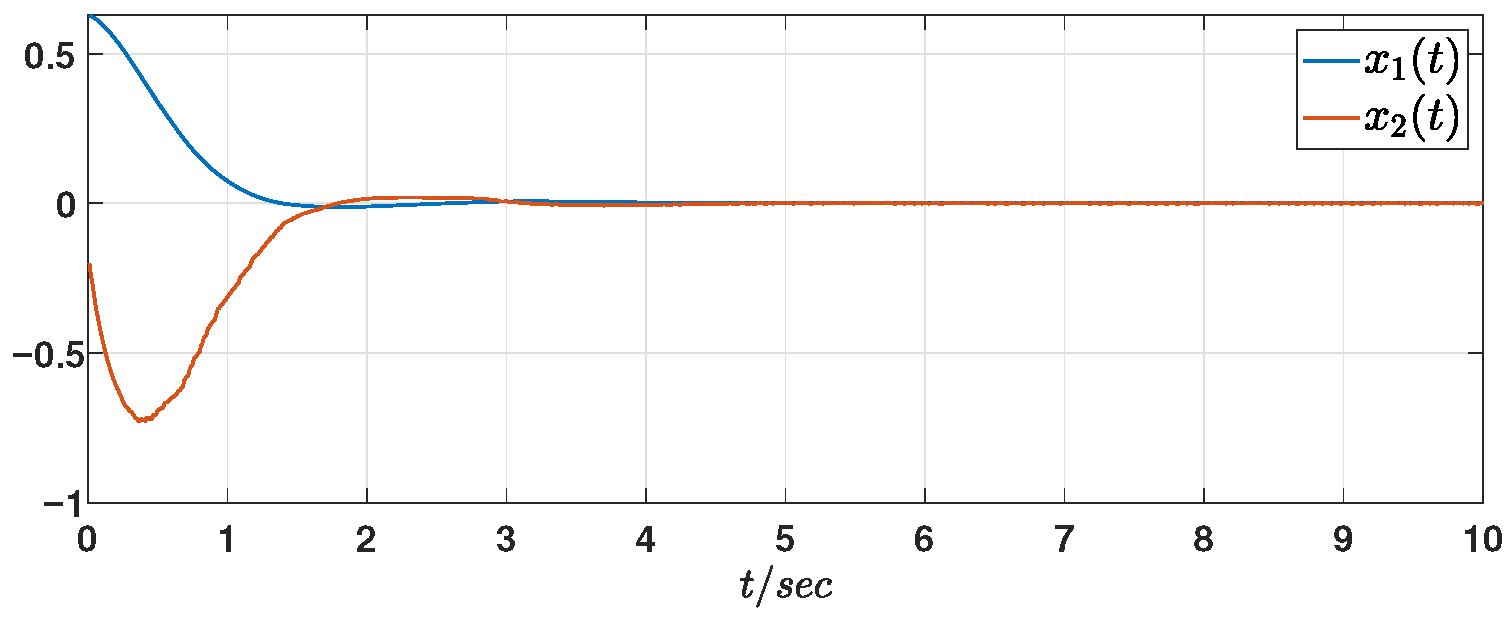
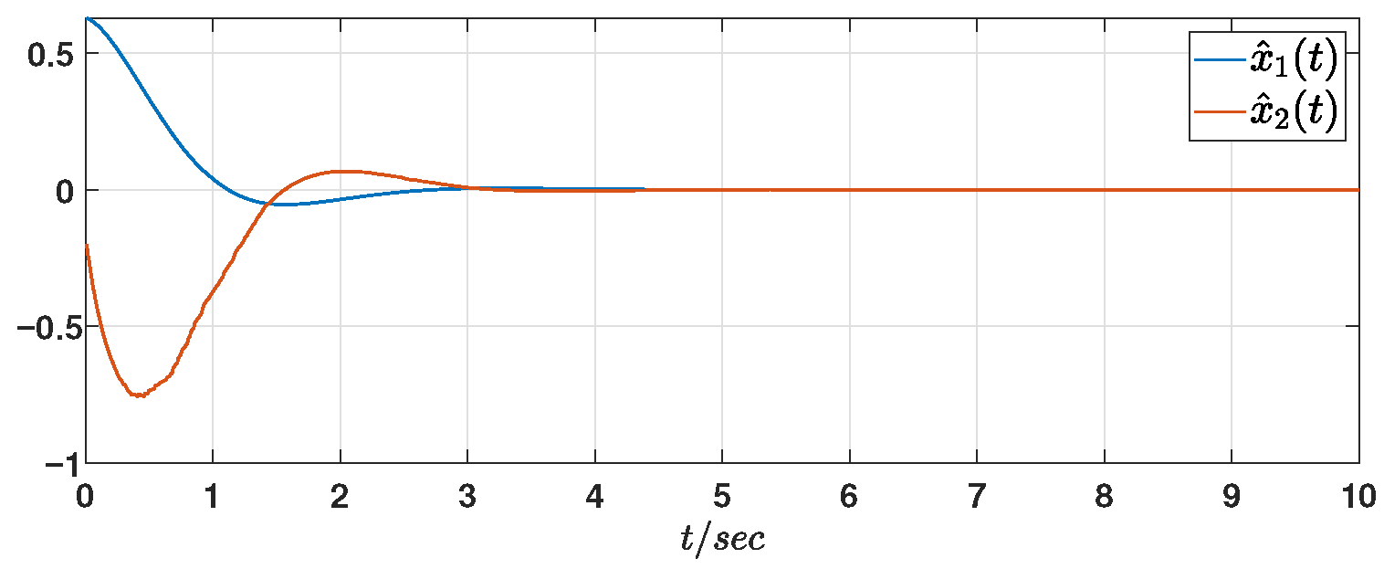
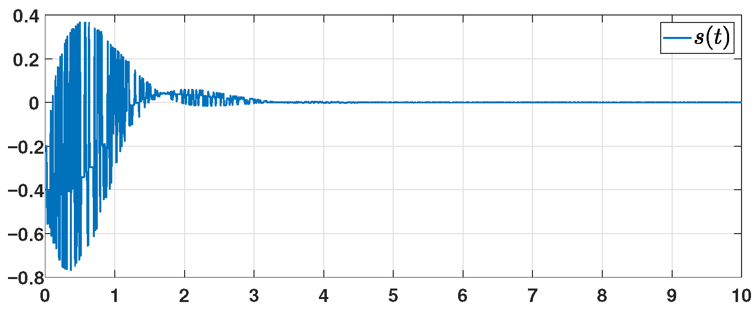
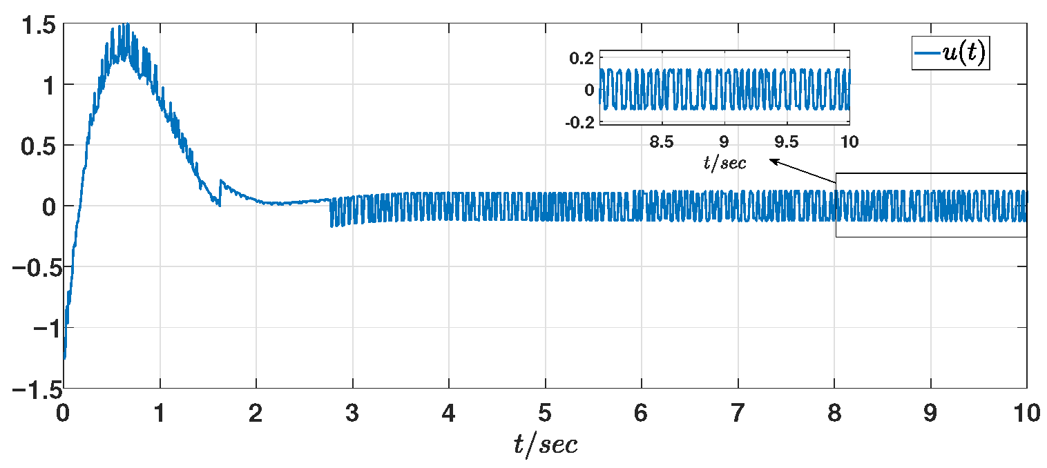
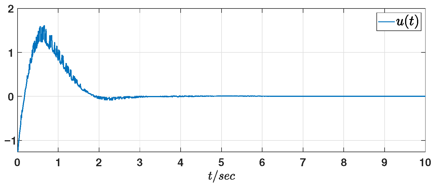
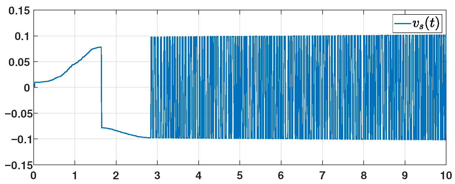
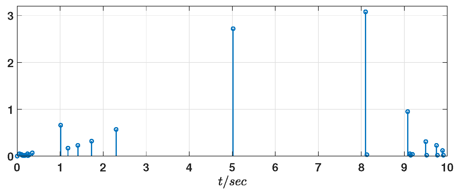
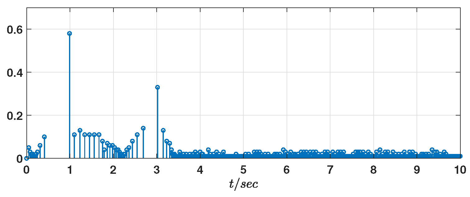
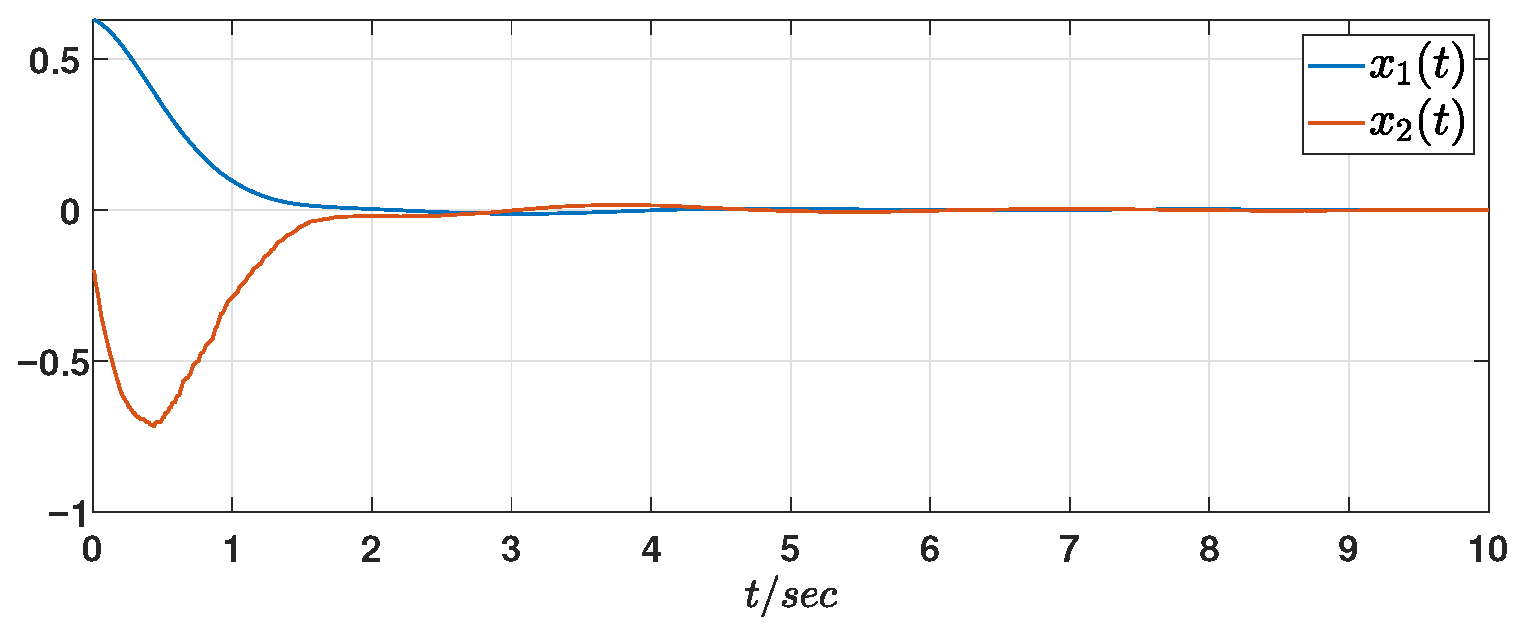
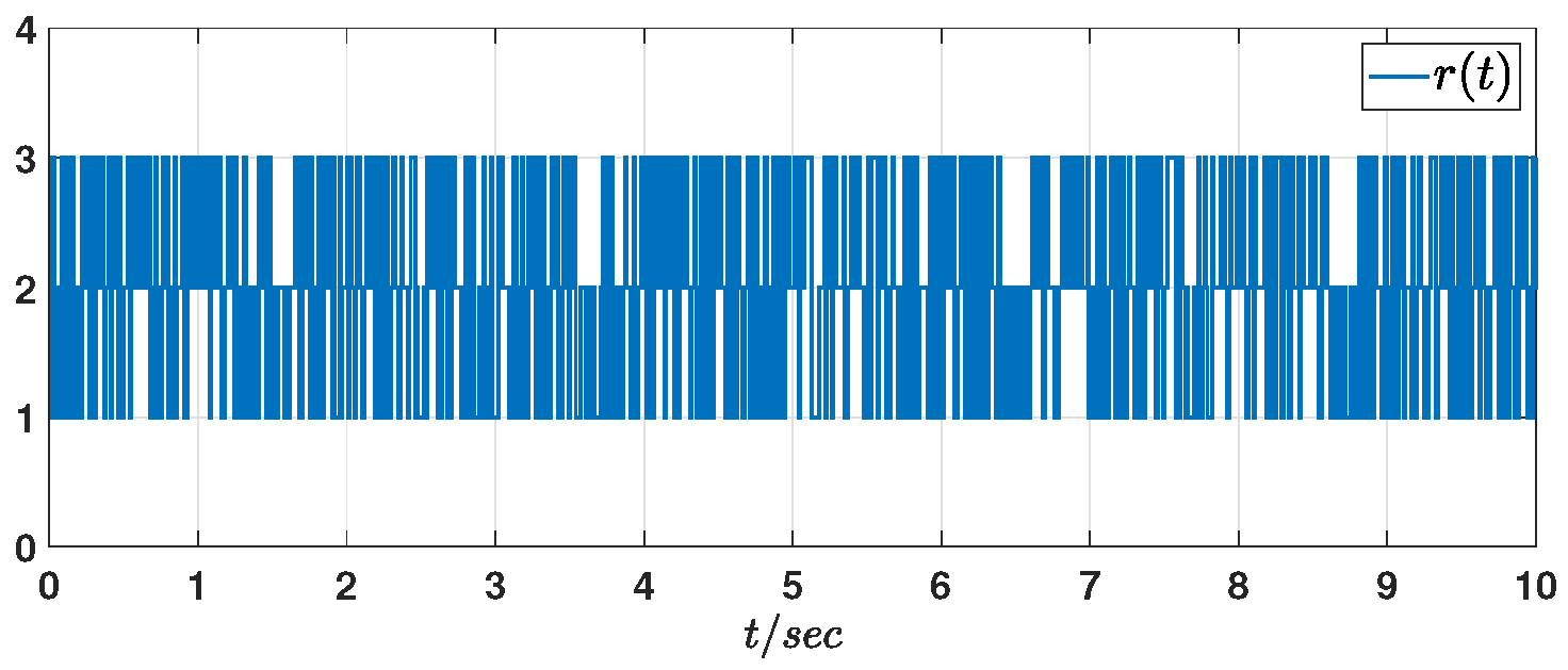
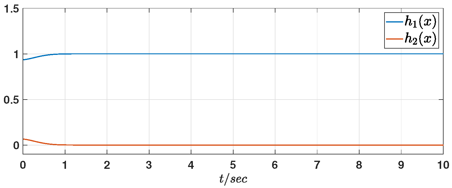
For simulation, set initial conditions as $x(0)=\widehat{x}(0)={[0.2\pi -0.2]}^T$. The parameters are chosen as $ϵ=\epsilon =0.01$, $\delta =0.1$, $\theta =0.5$, and $\psi (x(t),t)=0.1sin(x_1(t))$ represents the nonlinear function. The adaptive laws follow Equation (18), with parameters $c=10$ and $\Phi =I$. For the implementation of the neural network, the centers are set as $\mu =\left[\begin{array}{ccccc}-0.5& -0.25& 0& 0.25& 0.5\\ -0.5& -0.25& 0& 0.25& 0.5\end{array}\right]$, and the widths are given by $\sigma =[0.20.20.20.20.2]$. Simulation results are illustrated in Figure 1, Figure 2, Figure 3, Figure 4, Figure 5, Figure 6, Figure 7, Figure 8, Figure 9 and Figure 10. Figure 1 shows the evolution of the jumping modes. Figure 2 presents the fuzzy membership functions. Figure 3 and Figure 4 depict the state responses of the original system (1) and the observer system (6), respectively. The dynamic behavior of the sliding manifold is depicted in Figure 5. Variations in the control input signal are shown in Figure 6, which exhibits a severe chattering effect. To mitigate this issue, the switching signal $sgn(s(t))$ is replaced with $s(t)/(\parallel s(t)\parallel +0.01)$. As a result, the curve of the quasi-control input, shown in Figure 7, demonstrates a significant reduction in the chattering effect. Operational characteristics of the compensation mechanism are captured in Figure 8. Event-triggered instants and inter-event durations governed by the dynamic ETC strategy (5) are documented in Figure 9, in which 31 triggering events are detected. For comparison, a static ETC mechanism is also considered, in which the internal variable $\varpi (t)$ in Equation (5) is omitted. The corresponding result is shown in Figure 10, where 583 triggering events are observed. This comparison clearly demonstrates that the dynamic ETC mechanism achieves longer average event intervals, thereby improving network efficiency by nearly ${\displaystyle \frac{583-31}{583}}\approx 95\%$ over the observed interval. To make the comparison more transparent, we add the average inter-event time $\overline{\tau }={\displaystyle \frac{T_f-T_0}{N_{\mathrm{trig}}}}$, where $T_0=0$ and $T_f=10$ s denote the initial and final simulation times. Hence, ${\overline{\tau }}_{\mathrm{dyn}}=10/31\approx 0.323\mathrm{s},{\overline{\tau }}_{\mathrm{sta}}=10/583\approx 0.017\mathrm{s}.$ Consequently, the system requires fewer updates and communications, significantly reducing the number of triggering events and conserving communication resources.

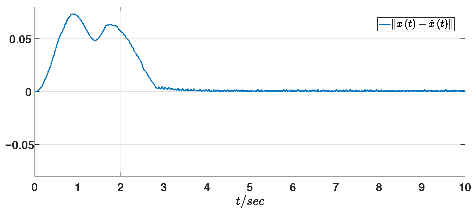
Furthermore, to evaluate the robustness of the neural compensator-based SMC, a simulation is conducted under the condition where no neural compensator is implemented. The resulting state response of the original plant, affected by unknown nonlinearities, is shown in Figure 11. Compared with the response shown in Figure 3, the proposed neural compensator-based SMC exhibits superior performance in terms of faster response, improved transient behavior, and better steady-state characteristics. Meanwhile, Figure 12 provided the variation trajectory of the $L2$-norm value of the system error, greatly improving the reliability and verifiability of the simulation.

Remark 4.

The communication load reduction is primarily due to the dynamic event-triggered structure, while the NN compensator modifies the closed-loop dynamics, but does not enter the triggering inequality, and therefore, it influences the event sequence only indirectly.

Remark 5.

The proposed dynamic event-triggered observer-based neural SMC method has significantly outperformed conventional SMC and non-event-triggered benchmark approaches across multiple aspects. By estimating unmeasurable premise variables through a state observer and reconstructing input matrices, it has overcome traditional SMCs’ strict requirements on measurable variables and specific input matrix structures. The incorporation of an RBF neural network-based online adaptive compensation mechanism has effectively suppressed unknown nonlinear disturbances, eliminating traditional SMCs’ dependence on disturbance boundaries and conservative gain selection. The dynamic event-triggered mechanism has extended the average triggering interval from 0.017 s in static mechanisms to 0.323 s, reducing the communication load by approximately $95\%$. The established LMI stability conditions have enabled handling of generally uncertain TRs, enhancing robustness in Markov jump systems. This method has demonstrated superior comprehensive control performance, robustness, and resource efficiency under multiple challenges.

5. Conclusions

This study proposed an event-triggered observer design methodology for neural SMCs in nonlinear T-S fuzzy MJSs with unmeasurable premise variables. To support observer synthesis, a dynamic ETC mechanism integrated with a neural network-based compensator was developed. An integral sliding surface was constructed to establish the coupled dynamics between the sliding mode and observation error, based on estimated premise variables. Building on this framework, novel stochastic stabilization conditions were derived, incorporating $H_{\infty }$ disturbance attenuation under uncertain TRs. In addition, a fuzzy adaptive SMC strategy was formulated to ensure finite-time convergence to the desired sliding surface. The effectiveness and practicality of the proposed approach were demonstrated through numerical simulations involving an industrial robotic manipulator. In the future, we will focus on relaxing theoretical assumptions, developing more efficient algorithms, and exploring more complex systems in which the TRs are highly uncertain or time-varying.

References

1. Takagi, T.; Sugeno, M. Fuzzy identification of systems and its applications to modeling and control. IEEE Trans. Syst. Man Cybern. 1985, SMC-15, 116–132. [Google Scholar] [CrossRef]
2. Zhao, N.; Zhao, X.; Zong, G.; Xu, N. Resilient event-triggered filtering for networked switched T-S fuzzy systems under denial-of-service attacks. IEEE Trans. Fuzzy Syst. 2023, 32, 2140–2152. [Google Scholar] [CrossRef]
3. Mimoune, K.; Hammoudi, M.; Hamdi, W.; Mimoune, S. Observer design for Takagi–Sugeno fuzzy systems with unmeasured premise variables: Conservatism reduction using line integral Lyapunov function. ISA Trans. 2023, 142, 626–634. [Google Scholar] [CrossRef]
4. Wu, Y.; Hu, S.; Li, W. Exponential stability of stochastic Takagi–Sugeno fuzzy systems under intermittent dynamic event-triggered control. IEEE Trans. Fuzzy Syst. 2022, 30, 1648–1659. [Google Scholar] [CrossRef]
5. Mao, D.; Ma, Y. Finite-time mixed H and passivity analysis for Takagi–Sugeno fuzzy system with time-varying delays and actuator faults. Commun. Nonlinear Sci. Numer. Simul. 2023, 116, 106770. [Google Scholar] [CrossRef]
6. Kchaou, M.; Mubeen Tajudeen, M.; Syed Ali, M.; Rajchakit, G.; Shanthi, G.; Cao, J. Asynchronous H control for IT2 fuzzy networked system subject to hybrid attacks via improved event-triggered scheme. Inf. Sci. 2024, 666, 120390. [Google Scholar] [CrossRef]
7. Zhuang, G.; Xia, J.; Feng, J.; Wang, Y.; Chen, G. Dynamic compensator design and H admissibilization for delayed singular jump systems via Moore-Penrose generalized inversion technique. Nonlinear Anal. Hybrid Syst. 2023, 49, 101361. [Google Scholar] [CrossRef]
8. Jiang, B.; Karimi, H.; Yang, S. Observer-based adaptive sliding mode control fo nonlinear stochastic Markov jump systems via T-S fuzzy modeling: Applications to robot arm model. IEEE Trans. Ind. Electron. 2021, 68, 466–477. [Google Scholar] [CrossRef]
9. Jiang, B.; Niu, F.; Wu, Z.; Qiu, J. Robust adaptive sliding mode security control of Markov jump cyber-physical systems with stochastic injection attacks through event-triggered-based observer approach. IEEE Trans. Syst. Man Cybern. Syst. 2025, 55, 3679–3692. [Google Scholar] [CrossRef]
10. Liang, X.; Bao, D.; Yang, Z. State evaluation method for complex task network models. Inf. Sci. 2024, 653, 119796. [Google Scholar] [CrossRef]
11. Wang, F.; Long, L. Switched-observer-based event-triggered adaptive fuzzy funnel control for switched nonlinear systems. IEEE Trans. Fuzzy Syst. 2022, 30, 1773–1787. [Google Scholar] [CrossRef]
12. Kchaou, M.; Jerbi, H.; Toual, B.; Kouzou, A. Non-fragile mixed H/passive-based asynchronous sliding mode control for nonlinear singular Markovian jump systems. Int. J. Syst. Sci. 2022, 53, 447–467. [Google Scholar] [CrossRef]
13. Wang, J.; Huang, Y.; Xie, X.; Yan, H.; Shen, H. Optimal control for fuzzy Markov jump singularly perturbed systems: A hybrid zero-sum game iteration approach. IEEE Trans. Fuzzy Syst. 2024, 32, 6388–6398. [Google Scholar] [CrossRef]
14. Wang, J.; Wu, J.; Shen, H.; Cao, J.; Rutkowski, L. Fuzzy H control of discrete-time nonlinear Markov jump systems via a novel hybrid reinforcement Q-Learning method. IEEE Trans. Cybern. 2023, 53, 7380–7391. [Google Scholar] [CrossRef]
15. Utkin, V.I. Sliding Modes in Control and Optimization; Springer Science & Business Media: Berlin/Heidelberg, Germany, 2013. [Google Scholar]
16. Tu, W.; Dong, J. Improved robust reduced-order sliding mode fault-tolerant control for T-S fuzzy systems with disturbances. Fuzzy Sets Syst. 2023, 464, 108481. [Google Scholar] [CrossRef]
17. Mani, P.; Joo, Y.H. Fuzzy logic-based integral sliding mode control of multi-area power systems integrated with wind farms. Inf. Sci. 2021, 545, 153–169. [Google Scholar] [CrossRef]
18. Sun, X.; Zhang, L.; Gu, J. Neural-network based adaptive sliding mode control for takagi-sugeno fuzzy systems. Inf. Sci. 2023, 628, 240–253. [Google Scholar] [CrossRef]
19. Kchaou, M.; Jerbi, H. Reliable H and passive fuzzy observer based sliding mode control for nonlinear descriptor systems subject to actuator failure. Int. J. Fuzzy Syst. 2021, 24, 105–120. [Google Scholar] [CrossRef]
20. Jiang, B.; Wu, Z.; Karimi, H.R. A distributed dynamic event-triggered mechanism to HMM sliding mode observer and H control of Markov jump systems. Automatica 2022, 142, 110357. [Google Scholar] [CrossRef]
21. Palanimuthu, K.; Kim, H.S.; Joo, Y.H. T-S fuzzy sliding mode control for double-fed induction generator-based wind energy system with a membership function-dependent H-approach. Inf. Sci. 2022, 596, 73–92. [Google Scholar] [CrossRef]
22. Zhu, J.; Zhuang, G.; Xia, J.; Xie, X. Dynamic memory event-based adaptive sliding mode control for networked nonlinear implicit hybrid systems under random spoofing attacks and data-buffer-aided mechanism. IEEE Trans. Control Netw. Syst. 2025, 12, 967–979. [Google Scholar] [CrossRef]
23. Yang, Y.; Niu, Y.; Lam, H.K. Sliding-mode control for interval type-2 fuzzy systems: Event-triggering WTOD scheme. IEEE Trans. Cybern. 2023, 53, 3771–3781. [Google Scholar] [CrossRef]
24. Jiang, B.; Gao, C. Decentralized adaptive sliding mode control of large-scale semi-Markovian jump interconnected systems with dead-zone input. IEEE Trans. Autom. Control 2022, 3, 1521–1528. [Google Scholar] [CrossRef]
25. Li, F.; Liu, Z.; Jiang, B. Adaptive finite-time fuzzy fractional sliding mode control for uncertain QUAV with actuator faults and slung load. IEEE Trans. Aerosp. Electron. Syst. 2025, 61, 3046–3058. [Google Scholar] [CrossRef]
26. Zong, G.; Wang, Y.; Niu, B.; Su, S.F.; Shi, K. Event-triggered adaptive NN tracking control for nonlinear systems with asymmetric time-varying output constraints and application to an AUVs. IEEE Trans. Veh. Technol. 2025, 74, 413–424. [Google Scholar] [CrossRef]
27. Xu, X.; Kao, Y.; Du, Z.; Zhao, X. Observer-based adaptive sliding mode control for Markovian jumping fuzzy systems with fractional brownian motions. IEEE Trans. Fuzzy Syst. 2024, 32, 2153–2163. [Google Scholar] [CrossRef]
28. Ge, X.; Han, Q.L.; Zhang, X.M.; Ding, D. Dynamic event-triggered control and estimation: A survey. Int. J. Autom. Comput. 2021, 18, 857–886. [Google Scholar] [CrossRef]
29. Wang, T.; Zong, G.; Zhao, X.; Xu, N. Data-driven-based sliding-mode dynamic event-triggered control of unknown nonlinear systems via reinforcement learning. Neurocomputing 2024, 601, 128176. [Google Scholar] [CrossRef]
30. Wu, Y.; Guo, Z.; Xue, L.; Ahn, C.K.; Liu, J. Stabilization of complex networks under asynchronously intermittent event-triggered control. Automatica 2024, 161, 111493. [Google Scholar] [CrossRef]
31. Ning, P.; Hua, C.; Li, K.; Meng, R. Event-triggered control for nonlinear uncertain systems via a prescribed-time approach. IEEE Trans. Autom. Control 2023, 68, 6975–6981. [Google Scholar] [CrossRef]
32. Zhang, Z.; Niu, Y. Sliding mode control of interval type-2 T-S fuzzy systems with redundant channels. Nonlinear Dyn. 2022, 108, 3579–3593. [Google Scholar] [CrossRef]
33. Wu, J.; Peng, C.; Yang, H.; Wang, Y.L. Recent advances in event-triggered security control of networked systems: A survey. Int. J. Syst. Sci. 2022, 53, 2624–2643. [Google Scholar] [CrossRef]
34. Zhuang, G.; Zhu, Q.; Xie, X.; Xia, J. Event-based H fuzzy control for implicit hybrid AVS systems embedding acceleration characteristic under random deception and DoS attacks. IEEE Trans. Autom. Sci. Eng. 2025, 22, 6154–6167. [Google Scholar] [CrossRef]
35. Shen, H.; Zhao, W.; Cao, J.; Park, J.H.; Wang, J. Predefined-time event-triggered tracking control for nonlinear servo systems: A fuzzy weight-based reinforcement learning scheme. IEEE Trans. Fuzzy Syst. 2024, 32, 4557–4569. [Google Scholar] [CrossRef]
36. Guan, C.X.; Fei, Z.Y.; Feng, Z.G.; Shi, P. Stability and stabilization of singular Markovian jump systems by dynamic event-triggered control strategy. Nonlinear Anal. Hybrid Syst. 2020, 38, 100943. [Google Scholar] [CrossRef]
37. Boukas, E. Stabilization of stochastic singular nonlinear hybrid systems. Nonlinear Anal. Theory Methods Appl. 2006, 64, 217–228. [Google Scholar] [CrossRef]
38. Wang, Y.; Xie, L.; de Souza, C.E. Robust control of a class of uncertain nonlinear systems. Syst. Control Lett. 1992, 19, 139–149. [Google Scholar] [CrossRef]
39. Wu, H.N.; Cai, K.Y. Mode-independent robust stabilization for uncertain Markovian jump nonlinear systems via fuzzy control. IEEE Trans. Syst. Man Cybern. Part B Cybern. 2006, 36, 509–519. [Google Scholar]
Figure 1. The Markov process.
Electronics 14 04758 g001
Figure 2. The membership functions.
Electronics 14 04758 g002
Figure 3. State response of original system.
Electronics 14 04758 g003
Figure 4. State response of observer.
Electronics 14 04758 g004
Figure 5. The sliding surface function s ( t ) .
Electronics 14 04758 g005
Figure 6. Control input u ( t ) .
Electronics 14 04758 g006
Figure 7. Quasi-control input u ( t ) .
Electronics 14 04758 g007
Figure 8. The curve for compensator.
Electronics 14 04758 g008
Figure 9. The triggering instants and interval under dynamic ETC mechanism.
Electronics 14 04758 g009
Figure 10. The triggering instants and interval under static ETC mechanism.
Electronics 14 04758 g010
Figure 11. State response of original system under non-neural SMC.
Electronics 14 04758 g011
Figure 12. The variation in L 2 -norm value of error.
Electronics 14 04758 g012