Signal Surface Augmentation for Artificial Intelligence-Based Automatic Modulation Classification

Abstract

Automatic modulation recognition has regained attention as a critical application for cognitive radio, combining artificial intelligence with physical layer monitoring of wireless transmissions. This paper formalizes signal surface augmentation (SSA), a process that decomposes signals into informative subcomponents to enhance AI-based analysis. We employ Bivariate Empirical Mode Decomposition (BEMD) to break signals into intrinsic modes while addressing challenges like adjacent trends in long sample decompositions and introducing the concept of data overdispersion. Using a modern, publicly available dataset of synthetic modulated signals under realistic conditions, we validate that the presentation of BEMD-derived components improves recognition accuracy by 13% compared to raw IQ inputs. For extended signal lengths, gains reach up to 36%. These results demonstrate the value of signal surface augmentation for improving the robustness of modulation recognition, with potential applications in real-world scenarios.

1. Introduction

1.1. Context

In the ever-evolving landscape of wireless communications, automatic modulation recognition (AMR) stands as a pivotal domain, strategically positioned at the intersection of signal processing, communication engineering, and artificial intelligence (AI). Automatic modulation classification (AMC), a sub part of AMR, refers to the automated process of identifying and categorizing the modulation schemes employed in captured signals. This capability holds paramount importance in the context of modern communication systems, where the efficient recognition of modulation types is essential for tasks ranging from spectrum monitoring and signal classification to adaptive signal processing.

The fundamental principle of AMR lies in its ability to discern the unique characteristics embedded within modulated signals, unraveling the distinctive fingerprints left by different modulation schemes on the received waveform. By harnessing advanced signal processing techniques, statistical analysis, and machine learning algorithms, AMR not only enables the automatic identification of modulation types but also contributes significantly to the optimization of communication system performance. Indeed, software-defined radios dynamically adjust their modulation according to external factors [1]. Accurate detection helps reduce control header overhead and minimizes unnecessary exchanges. The relentless advancement of communication technologies, including the appearance of diverse modulation schemes and signal complexities, underscores the ongoing importance of AMR in ensuring robust and adaptive communication networks.

1.2. State of the Art

AMC has long been a subject of interest, with notable contributions, including a foundational reference book authored by Zhu and Nandi [2]. Traditionally, two primary modulation classification approaches have prevailed: the decision–theoretic approach and the feature-based approach. However, the landscape of AMC has experienced a revitalization with the emergence of deep learning architectures. Recent surveys such as those presented in [3,4] provide a comprehensive overview of various AMC methods, encompassing both traditional and contemporary classification approaches. To the best of the authors’ knowledge, the application of Bivariate Empirical Mode Decomposition (BEMD) in telecommunications signals, proposed in this work, is a relatively uncommon practice, with minimal representation in recent surveys and the literature.

Yet, as demonstrated by the authors of [5], decomposing the IQ (in phase and in quadrature) signal using BEMD before feeding the result into a convolutional neural network (CNN) enhances feature extraction and improves classification accuracy. However, while BEMD decomposition effectively extracts scales, it is slow and computationally intensive. In this context, “scale” denotes the intrinsic time-frequency characteristics of each decomposed component, with fine scales corresponding to high-frequency, short-duration features and coarse scales to low-frequency, long-duration variations. There is thus a trade-off to make between an increase in classification rate and decomposition time, which depends on the complexity of the decomposition method.

The contributions of this paper are multifaceted. First, the authors’ previous research is validated using a more realistic, publicly available dataset. Second, the algorithmic implementation of the BEMD decomposition is enhanced for greater efficiency and accuracy. Lastly, two new concepts are introduced: signal surface augmentation (SSA) and adjacent trends (ATs). SSA is the action of decomposing the original signal into distinct components, therefore expanding the feature space to provide the AI model with a richer, more informative input for improved recognition performance. Adjacent trends refer to scales that emerge in longer waveforms but lack meaningful information. The improved algorithm mitigates the impact of these trends, thereby reducing the number of input nodes required and shortening the training time of the network. This combination of SSA and AI effectively increases the available surface, unfolding the signal into an expanded and more informative feature space.

To achieve this objective, the following sections of this article first provide detailed information on the databases used, the methodology employed, and the architecture designed for this study (Section 2). In Section 3, the concept of signal surface augmentation is introduced. Section 4 presents the fundamentals of BEMD decomposition, followed by the description of different enhancements. Finally, the results are presented and discussed in Section 5.

2. Insights into the Employed IQ Databases

2.1. O’Shea’s RadioML2016a Dataset

In the pursuit of classifying a wide range of modulations, the foundation lies in having a comprehensive IQ samples database of modulated signals. For this purpose, the adopted dataset in the authors’ previous publication [5] is O’Shea’s renowned RadioML2016a dataset [6], which also serves as a reference dataset in this paper. This publicly available dataset comprises complex-valued IQ samples, each spanning 128 samples and encompassing a diverse range of radio signal modulations. It has become a staple in research focused on automatic modulation classification and Machine Learning (ML) for signal processing, facilitating performance comparisons in the field [7,8].

The RadioML2016a dataset serves as a valuable resource for researchers and developers actively engaged in crafting new algorithms for radio signal classification. The dataset encompasses single-carrier modulations like, e.g., GFSK (Gaussian Frequency Shift Keying), 64QAM (Quadrature Amplitude Modulation), WBFM (WideBand Frequency Modulation), and QPSK (Quadrature Phase Shift Keying). With a total of 11 modulation schemes and signal-to-noise ratios ranging from −20 dB to 18 dB in 2 dB increments, it provides a dataset of 220,000 waveforms, with each waveform consisting of 128 samples.

O’Shea’s dataset [6,9], is often considered the gold standard for telecommunication signals in the field of this paper. Despite the acknowledged flaws and curiosities [10], such as the SNR dB values [11], the use of variance instead of standard deviation, and the error in the noise amplitude calculation (a factor of 2), it remains freely accessible. Additionally, its widespread use in previous studies makes performance comparisons possible.

2.2. Spooner’s CSPB.ML.2018 Dataset

The CSPB.ML.2018 Dataset [12] also used in this paper is employed in [13,14]. In [13], CAPsule networks (CAP) are combined with raw IQ data, whereas [14] investigates their integration with Cyclic Cumulant (CC) features, which are extracted through blind estimation using Cyclostationary Signal Processing (CSP). These CC features are subsequently employed for training and classification within the CAP framework. The dataset has also been used in [15,16] for automatic modulation recognition.

This paper also utilizes the dataset to validate the advantages of decomposing the signal before injecting it into the AI architecture, as well as to assess how the methodology performs with long data sequences. The dataset comprises 112,000 waveforms featuring eight modulation types: BPSK (Binary Phase Shift Keying), QPSK (Quadrature Phase Shift Keying), 8PSK, ${\displaystyle \frac{\pi }{4}}$-DQPSK (Differential Quadrature Phase Shift Keying), 16QAM (Quadrature Amplitude Modulation), 64QAM, 256QAM, and MSK (Minimum Shift Keying). It exclusively includes digital single carrier modulations. Each waveform is associated with a file containing nine parameters: signal index, signal type, base symbol period, carrier offset, excess bandwidth, up and down sampling factors, in-band signal-to-noise ratio (SNR) in dB, and noise spectral density in dB.

The reasoning for expressing noise spectral density in dB rather than in units like W/Hz or dBW/Hz stems from the assumption that, for this dataset and most signal-processing applications, the signals are treated as if the sampling rate is unity, $f_s=1$. Under this assumption, the variance of the noise sequence, ${\sigma }_n^2$, is equivalent to the spectral density $N_0$ in Watts/Hz:

$$R_n^0\left(0\right)={\sigma }_n^2={\int }_{-1/2}^{1/2}{N}_{0}df=N_0$$

(1)

In this context, the noise variance is unity by default, which implies that the noise spectral density is also unity, as $f_s=1$. This approach is particularly useful in RF signal processing, where sampled data is common. By assuming $f_s=1$, both code and equations for processing the data can be written more conveniently. Scaling by the physical value of the sampling rate is then applied at the end, when reporting time or frequency, to reflect real-world measurements.

Regarding the sampling factor, the actual symbol rate of the signal in the file is calculated using the base symbol period $\left(T_0\right)$, the upsample factor (U), and the downsample factor (D):

$$f_{sym}={\displaystyle \frac{1}{T_0}}\ast {\displaystyle \frac{D}{U}}.$$

(2)

Table 1. CSPB.ML.2018 Dataset Parameters [12].

Parameter	Range/Values
Modulations	BPSK, QPSK, ${\displaystyle \frac{\pi }{4}}$-DQPSK, 8PSK,
	MSK, 16QAM, 64QAM, 256QAM
Base symbol period	1–15 samples
Carrier freq. offset (norm.)	$[-{10}^{-3}, {10}^{-3}]$ cycles sample−1
Roll-off factor	0.1–1
SNR	−2 to 12.8 dB
Up/down sampling	(1,1), (3,2), (4,3) → (10,9)
Noise spec. density	0 dB
Signal length	32,678 samples
Number of waveforms	112,000

lists the parameter ranges of the dataset. The waveforms have a length of 32,768 samples. This extended length is a deliberate choice by the creator, who focuses on cyclostationary features. The increased number of samples is essential for extracting Cyclic Features (CFs). This characteristic not only allows for in-depth analysis of the impact of decomposition on large datasets but also presents an opportunity to enhance automatic modulation recognition.

The synthetic dataset used in this study is intentionally generic and does not assume a fixed sampling frequency. The signals are represented as normalized IQ vectors, and the effective sampling rate scales with the modulation bandwidth, which typically yields between one and fifteen samples per symbol. Because the dataset is normalized and does not explicitly model channel effects, the absolute sampling frequency is not required for training or evaluation. The signals contained in the database may therefore represent either narrowband or wideband scenarios, including satellite communication links, although spread spectrum techniques are not included. For context, widely used datasets such as the narrowband dataset of O Shea and collaborators operate at sampling frequencies on the order of one megahertz (see Ref. [9]). Under these conditions, the SSA approach appears insensitive to the sampling parameters. However, its behavior on real-world RF signals cannot yet be predicted since additional noise sources and channel impairments depend explicitly on the bandwidth and on the sampling frequency. The underlying principles of SSA remain the same, and BEMD decomposition can still be applied. When the algorithm is unable to extract meaningful structure from the signal, the corresponding content is naturally absorbed into the final intrinsic mode function, that is, the residual component.

2.3. Dataset Comparison

Both datasets are generated synthetically: CSPB.ML.2018 using MATLAB (R2018a) and RadioML2016a through GNURadio (V 3.7.9). Both employ a Nyquist filter for digital modulations, with varying roll-off factors for CSPB.ML.2018 and a fixed roll-off factor for RadioML2016a of 0.35.

Table 2. Dataset comparison.

Characteristic	O’Shea [6]	Spooner [12]
Modulations	11	8
Analog	yes	no
# samples per waveform	128	32,768
Applied CFO	Yes std: 0.01 max: 500 in Hz	yes
Varying symbol length	no	yes
SNR [dB]	−20 to 18 (erroneous)	−2 to 12.8
# waveforms	220,000	112,000
File type (binary)	1 .pkl	28 .tim
Flaws	yes, reported	unknown
Widely adopted	yes	not yet

compares the key characteristics of both datasets. It is important to note that Spooner’s CSPB.ML.2018 dataset does not include analog modulations, such as amplitude and frequency modulations. This omission is not critical, as modern communications primarily rely on digital methods, and analog modulations can often be more easily identified through amplitude and phase deviation measurements. Additionally, the CSPB.ML.2018 dataset offers significantly more samples per waveform, and there is greater variation in roll-off factors and Carrier Frequency Offset (CFO). The CSPB.ML.2018 dataset avoids excessively low (negative) SNR values, which aligns with realistic scenarios. Extremely low SNR levels would render signal detection impossible, making such conditions unrealistic for practical applications. Additionally, the dataset includes high order digital modulations, such as 256QAM, which, when combined with OFDM, aligns it more closely with modern requirements like 5Gs enhanced Mobile Broadband eMBB use cases.

3. Signal Surface Augmentation

In this section, we begin by defining the concepts of signal surface augmentation and data shape, which are the core concepts of this article. We then clarify what SSA does not cover and what it should not be confused with. After that, we address the problem of data overdispersion, and finally, we highlight the main advantages of using SSA.

In a nutshell, SSA is a framework where, instead of feeding the raw signal directly into a network, we first expand the input signal surface by decomposing the signal. The more meaningful the decomposition and the better the resulting scales, the more effectively the network can absorb relevant information. By offering more opportunities to extract features, SSA improves classification performance without leading to overfitting.

3.1. Understanding Data Shape

The data shape inherently depends on the nature of the signal and the measurement process. It represents the structure of the measured signal and serves as the foundation for defining the input requirements of an AI architecture.

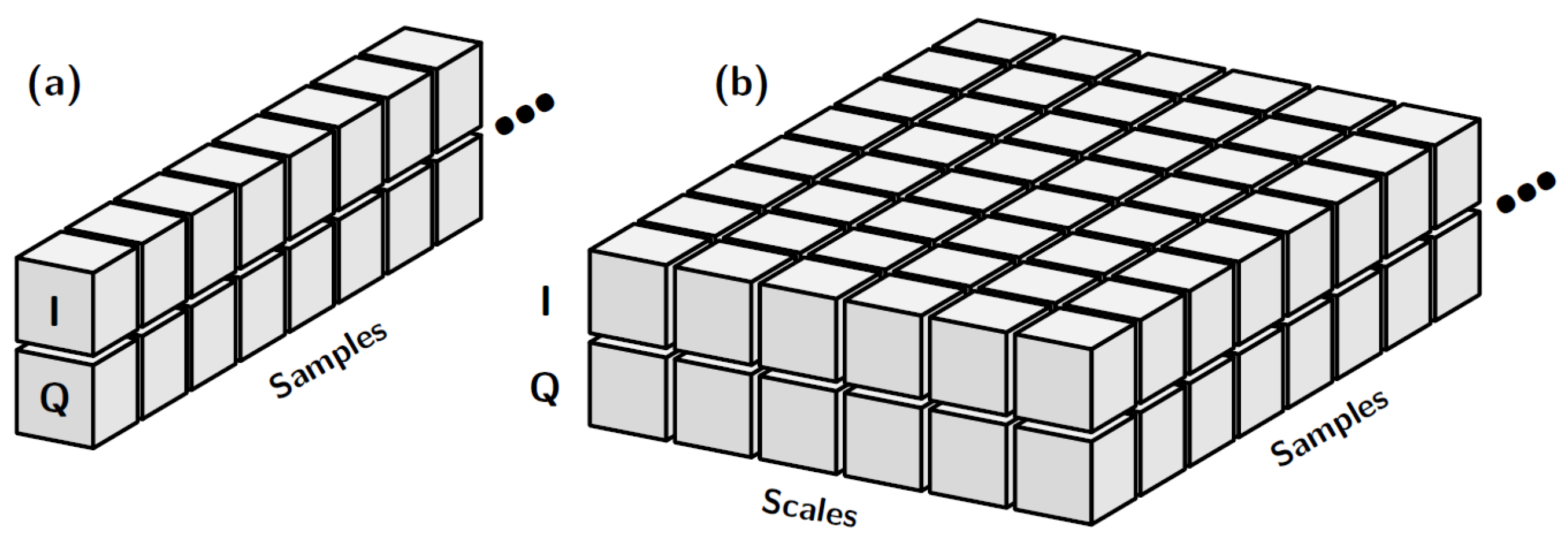
In this paper specific case, the data shape is typically multidimensional (see Figure 1b), encompassing three primary dimensions:

• Length: Represents time or the number of samples in the data.
• Height: Corresponds to the number of rows which, for an IQ signal, typically consists of two rows, one for the in-phase (I) component and one for the quadrature (Q) component (see Figure 1a).
• Depth: Indicates the number of channels or scales, which is often 1 but may vary depending on the analysis context (e.g., the number of decomposed scales in a multi-scale representation).

Defining the data shape is crucial to ensure compatibility with the AI model’s input requirements, enabling proper feature extraction and efficient processing. For IQ signals, this structured representation allows the model to leverage both the temporal characteristics of the data and the distinct properties of its I (In-phase) and Q (Quadrature) components.

Before data can be introduced into an AI architecture, it must undergo preprocessing to ensure it conforms to the correct data type and input shape required by the ML model. Many of the most powerful AI architectures have been designed primarily for tasks like image analysis, segmentation, or natural language processing (NLP), including generative AI applications. As a result, the data often needs to be transformed to align with these architectures.

For image-based models, this typically involves converting the data into a format resembling an image, such as a full three-channel RGB image with a specific resolution, or a single-channel matrix (greyscale image). For NLP models, the data might instead be transformed into vectors via tokenization. This preprocessing step is crucial to bridge the gap between the original dataset and the input requirements of these advanced AI systems.

In telecommunications, the most commonly used measurement is the IQ signal, a form of complex data that is typically represented as a 2 by x matrix (see Figure 1a, where x denotes the number of saved samples per waveform. However, to leverage the aforementioned AI architectures, the IQ signal must be transformed to fit the required input shape.

One approach involves creating square or rectangular image-like representations of the signal using techniques such as Fast Fourier Transform (FFT), waterfall spectrograms, eye diagrams, vector diagrams (constellation plots), and others. These methods effectively change the representation of the data to make it compatible with image-based architectures.

Alternatively, if the same IQ signal is used without such transformations, the architecture itself must be adapted. This entails modifying the input layer to accommodate the raw signal format and retraining the model entirely. In this scenario, transfer learning requires significant adaptation, as directly using a pretrained model becomes infeasible without extensive modifications.

3.2. What SSA Is Not

3.2.1. Multi-Scale Network Architectures

Multi-scale convolutional neural network-based methods involve processing input data through multiple pathways, each applying different kernel sizes to extract features at varying scales. These multi-scale features are then combined within the network, as demonstrated in works such as [17,18]. Alternatively, scaling can also be achieved through wavelet-based encoder–decoder architectures, as explored in [19].

In multi-scale CNNs, scaling is achieved by varying the kernel sizes, which effectively analyze the input signal within windows of different dimensions. This approach contrasts with signal surface augmentation, where scaling is performed through a meaningful signal decomposition process prior to introducing the data into the network. By decomposing the signal beforehand, SSA provides a structured and interpretable method for scaling, which enhances the network’s ability to extract relevant information without relying solely on in-network operations like kernel-based scaling.

3.2.2. Multimodal Fusion Approach

Multimodal refers to the integration and processing of data or information from multiple modes or types of input variables. A mode, in this context, refers to a distinct way of representing information, such as text, images, audio, video, or sensor data. Multimodal systems combine and analyze these different types of data to improve understanding, decision-making, and user experience. Multimodal systems aim to mimic how humans process and combine diverse information sources such as vision and sound at the same time, leading to more intuitive, accurate, and capable technologies. Unlike the multimodal approach, which involves multiple different data types, the SSA approach of this paper considers multiple modes within the same data, as it is a decomposition of a single data type.

3.2.3. Only Increasing the Number of Parameters in the First Expansion Layer

Increasing the input shape typically results in more trainable parameters at the beginning of the architecture. Conducting an empirical comparison using the architectures from [6] as a reference and extending the methodology presented in our previous work [5], we compare an original IQ model with 2,830,427 trainable parameters to a 3D-shaped BEMD model with 2,835,803 trainable parameters, revealing a slight increase in parameters. To further explore the concept of data presentation that we refer to as signal surface augmentation, we consider adjusting the number of filters in the first convolutional layer:

• Increasing the number of filters in the original architecture from 256 to 300 raises the trainable parameters to 2,851,723 but does not improve accuracy.
• Reducing the filters in the BEMD model from 256 to 200 decreases the parameters to 2,807,523, resulting in a slight absolute accuracy drop of 0.4%. This value is small, as it falls within the standard deviation of various cross-validation trainings, which is just under 1%.

In this example, while the IQ approach has more trainable parameters compared to the decomposition method, it yields worse results. The decomposition method is more effective at extracting features. Interestingly, the number of parameters in the input layer has minimal impact on the final accuracy.

3.2.4. Data Augmentation

Data augmentation [20] is a technique used to artificially expand a dataset by applying transformations such as rotation, scaling, flipping, or adding noise. It helps improve model generalization, especially in machine learning and deep learning, by making the model more robust to variations in data. Our approach does not increase the dataset by altering existing data; instead, it enhances feature visibility through decomposition.

3.3. Data Overdispersion: The Inversed Bottleneck Issue

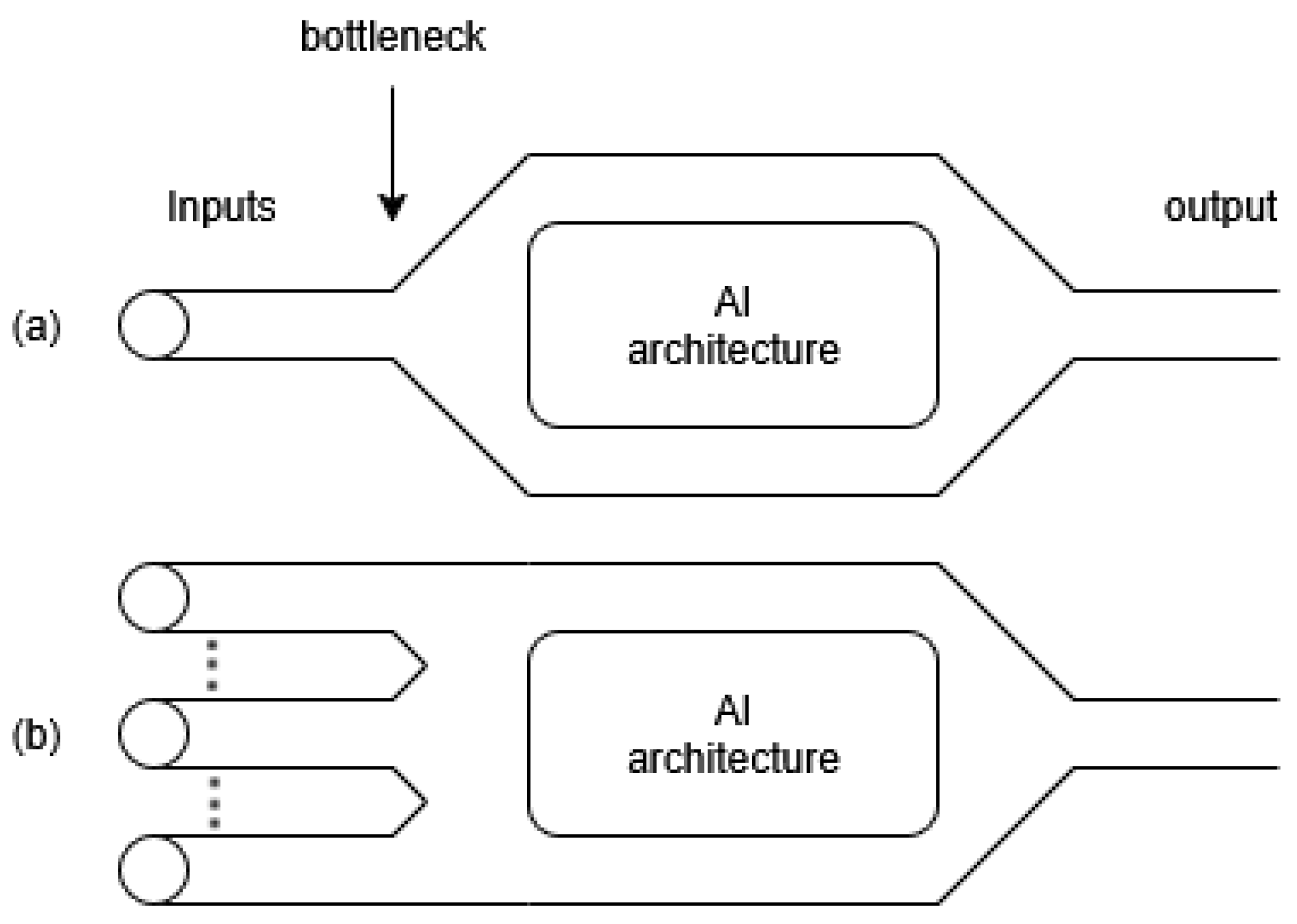
In artificial intelligence, the relationship between neural network design and input data is crucial to achieving optimal performance. One of the primary challenges in this domain is balancing model size with the nature of the input data. Overparameterization, for example, arises when a neural network has more parameters than necessary relative to the data available. This imbalance often leads to inefficiencies, as the network’s large capacity remains underutilized. A related issue, underutilized capacity, refers to scenarios where large models are applied to small datasets, resulting in wasted resources and the inability to fully leverage the network’s potential.

A new concept related to these ideas and introduced in this work is data overdispersion, which arises as a consequence of overparameterization and underutilized capacity. This phenomenon occurs when input information is spread too thinly across the network, making it difficult to maintain meaningful signal propagation. The dispersion of data causes the model to lose focus on the most critical patterns, diluting their significance and hindering effective learning.

When the network is disproportionately large compared to the input data, several challenges emerge. For instance, meaningful patterns in the data may become diluted as they are spread across too many neurons, weakening the network’s ability to amplify the most relevant features. Additionally, excessive capacity can lead to overfitting, where the model memorizes specific patterns rather than generalizing effectively to unseen data. Moreover, applying a large network to small data is computationally inefficient, as the added complexity does not provide proportional benefits and may even amplify noise, reducing the model’s reliability.

To address these challenges, researchers use a variety of techniques. Regularization methods, such as dropout or weight constraints, are common strategies to prevent overfitting by limiting the model’s ability to focus excessively on specific data points. Another approach is to design optimized architectures that align with the scale and complexity of the input data, ensuring that the network’s capacity is efficiently utilized. In some cases, data augmentation techniques such as cropping, rotation, or synthetic data generation can increase the amount of training data, helping to balance the relationship between model size and input. However, data augmentation is not always feasible, particularly for specialized or constrained datasets. For instance, datasets in fields like medical imaging, rare signal modulation types, or specific industrial sensor readings often cannot be artificially expanded due to their unique or highly specific characteristics.

Ultimately, the balance between model size and input data plays a vital role in building efficient and effective neural networks. Addressing issues like overparameterization, underutilized capacity, and data overdispersion is critical for achieving robust performance, especially in scenarios with limited data. By tailoring architectures, employing regularization, and augmenting data where possible, we can ensure that AI systems are both powerful and resource-efficient.

In Vision Transformers (ViTs), the process differs significantly. A large image is divided into smaller patches, which are then used to apply attention mechanisms. This approach allows the model to focus on various parts of the image simultaneously.

In contrast, telecommunications IQ signals present a different challenge; instead of extracting smaller patches from a larger dataset, we use SSA to decompose the IQ data into meaningful scales. This decomposition increases the size of the input, providing more granular information for the model to process. This process is not as straightforward as patch selection in ViTs as the data is transformed into multiple scales that add complexity to the input structure.

3.4. SSA

By combining all of these concepts, we can address data overdispersion while improving information extraction through the application of signal surface augmentation. In this process, we leverage decomposition scales to transform the data shape, effectively increasing its surface area for better analysis by AI architectures (see Figure 2).

The data shape is expanded using a decomposition technique, in this case, bivariate empirical mode decomposition. This method separates the input signal into intrinsic mode functions (IMFs), and when all of these IMF scales are summed, they reconstruct the original signal (see Equation (3)). This ensures that no information is lost during decomposition while also enabling a more nuanced representation of the data.

Additionally, this approach aligns well with the capabilities of classical convolutional neural networks. CNNs operate across all input channels, making them particularly effective for analyzing the decomposed scales. By assigning different weights to each scale during training, the architecture can prioritize the most informative parts of the data, amplifying relevant features and filtering out less useful ones. This dynamic weighting further enhances the model’s ability to extract meaningful patterns from the input.

The findings in Section 3.2 and Section 3.2.3 indicate that while changes in the initial input shape minimally impact the overall number of parameters in large architectures, significant accuracy gains are driven by the additional information within each channel of the data tensor. The increase in accuracy is not due to a rise in the number of trainable nodes in the input layers; this increase is negligible compared to the overall architecture size. Rather, the true advantage lies in the data shape achieved through decomposition, which enhances the architecture’s learning effectiveness.

Interestingly, although the initial information remains the same (IQ samples), providing the AI architecture with a ’larger canvas’, created via a number of dependent representations of the IQ signal, leads to a noticeable increase in final accuracy. We term this phenomenon “increasing the data or the signal surface”.

Indeed, decomposing the signal or applying spectral filtering, similar to techniques used with RGB images, can enhance the visibility of important information before filters extract the most valuable features.

The CNN kernels progressively extract higher-level and more abstract features as the depth of the network increases. This is wanted in image classification as kernels in the early layers of a CNN typically extract low-level features such as edges, textures, and simple patterns and also reduce the sizes of the intermediate outputs. If the telecommunication signals have high variability and contain fine-grained details, there is a risk that these initial layers might not capture all the necessary nuances, potentially leading to a loss of important information for modulation classification.

A common solution involves employing smaller kernel sizes in the early layers to enhance the capture of fine details and high-frequency variations, making it easier to detect subtle changes in the signal, while increasing the number of convolutional layers early in the network helps progressively capture detailed features, ensuring that crucial nuances in the signal are preserved.

These techniques are computationally more expensive but can be improved by using filtering techniques and multi-scale convolutional approaches can help capture features at different resolutions. This involves processing the signal at multiple scales to ensure that both fine and coarse features are captured effectively.

Instead of integrating them directly into the AI architecture, considerably increasing its size, we prepare them in advance by creating a 3D signal containing the scales. By processing the input data at multiple resolutions or scales, the network captures a wide range of features, from small, fine grained details to larger, more abstract patterns.

Integrating information from different scales enables the network to build a more comprehensive understanding of the input data. To achieve this, we construct a higher-dimensional input tensor, applying the approach directly at the data level rather than modifying the architecture itself. Again, we refer to this process as signal surface augmentation.

Signal surface augmentation can be used with any decomposition. However, we found two attributes that should be included in the chosen decomposition for the case of a standard CNN architecture and a multidimensional (3D) tensor:

• It should be possible to retrieve the original signal from the decomposed elements (e.g., such as adding the decompositions together).
• The number of extracted elements should be kept to a manageable quantity; we obtain good results with six to eight scales. Excessively large numbers of elements or nodes place additional demands on the hardware, as complex decompositions can be time-consuming and resource-intensive as well as increase training time.

The following section provides a detailed explanation of the selected decomposition algorithm in this paper and the subsequent improvements implemented.

4. An Improved Bemd Version for AMC

4.1. Empirical Mode Decomposition (EMD)

Huang et al. [21] introduced empirical mode decomposition (EMD) as the first part of a process for spectral analysis of time series. This approach does not need an a priori defined basis but uses data-driven basis functions. It is nowadays increasingly used in various domains, mainly for biomedical applications such as EEG (ElectroEncephaloGram), ECG (ElectroCardioGram) analyses, or natural phenomena analyses such as atmospheric, oceanic, or seismic studies. It is also used for mechanical applications (vibrations) and in image and speech processing [22].

The EMD methodology is suitable for non linear and non-stationary signals that are typical features of real telecommunication signals [23,24].

The decomposition mechanism, also called sifting, consists in decomposing the input signal $s\left(t\right)$ into a finite number M of IMFs such that the signal can be expressed as

$$s\left(t\right)=\sum _{i=1}^M{IMF}_i\left(t\right)+r\left(t\right)$$

(3)

where $r\left(t\right)$ is the residue which may or may not have a linear trend.

4.2. Bivariate Empirical Mode Decomposition (BEMD)

However, EMD is limited to univariate, real-valued data, whereas many modern datasets are bivariate, for example, complex signals such as baseband telecommunications signals demodulated via an IQ demodulator. As a result, researchers have worked on extending EMD to handle bivariate and even multivariate data types. This issue has received great interest in the scientific community, and a plethora of methods have been proposed for multivariate EMD decomposition [25,26,27,28,29,30].

In the context of this paper, telecommunication data series are primarily represented as complex IQ samples, which necessitate the use of bivariate empirical mode decomposition. This is particularly relevant in the realm of software-defined radio, where signals are inherently processed as IQ samples to preserve both amplitude and phase information.

BEMD decomposes a signal into components representing slower and faster oscillations. In the case of complex-valued signals, such as IQ data in telecommunications, these oscillations correspond to variations in amplitude and phase, which can be visualized as time-dependent rotating trajectories in the IQ plane.

These rotating components are extracted using the envelopes’ mean, requiring the signal’s projection onto various directions (N), or planes. After projection, the standard EMD method is applied to the 2D signal, allowing the extraction of finer details like amplitude and angular frequency. In our approach, we transform the initial 2D signal tensor into a 3D tensor by placing the separated IMFs into different channels, which is then used as input to the AI architecture.

The used algorithm [27], illustrated in Algorithm 1, presents the pseudocode for one sifting process in the BEMD method. This algorithm processes the complex IQ signal, denoted by $x\left(t\right)$, using a set of N projection angles ${\phi }_k$ (where $k=1,2,\dots ,N$). The projections of $x\left(t\right)$ onto these angles are given by $p_{{\phi }_k}\left(t\right)$. The pairs $(t_j^k,x(t_j^k))$ represent the time positions (or samples) and the local maxima points of the signal at those samples. The interpolated envelope curve, constructed from the maxima points for each projection angle ${\phi }_k$, is represented by $e_{{\phi }_k}\left(t\right)$. Finally, the mean trajectory of all the envelope curves is denoted by $m\left(t\right)$. 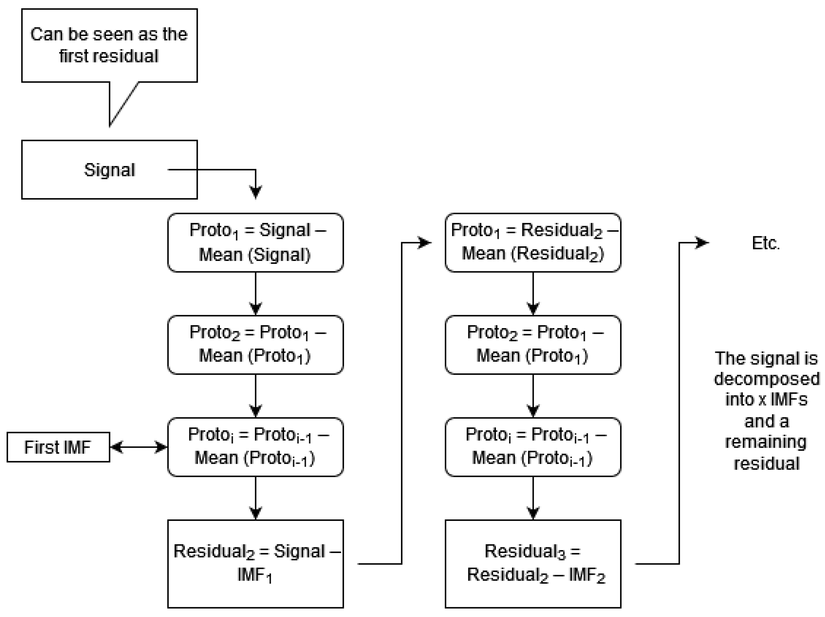The overall sifting process is further illustrated in Figure 3.

Algorithm 1 The used BEMD algorithm from [27]—case of 1 sifting

for  $1\le k\le N$  do         Project the complex valued signal $x\left(t\right)$ on direction ${\phi }_k$ (Plane P)         $\to p_{{\phi }_k}\left(t\right)=Re(e^{-i{\phi }_k}x\left(t\right))$           Extract the locations $\left[t_j^k\right]$ of the maxima of $p_{{\phi }_k}\left(t\right)$         Interpolate the set $(t_j^k,x(t_j^k))$ to obtain the envelope curve in direction ${\phi }_k:e_{{\phi }_k}\left(t\right)$ end for Compute the mean of all envelope curves $m\left(t\right)={\displaystyle \frac{1}{N}}{\sum }_k{e}_{{\phi }_k}\left(t\right)$ Subtract the mean

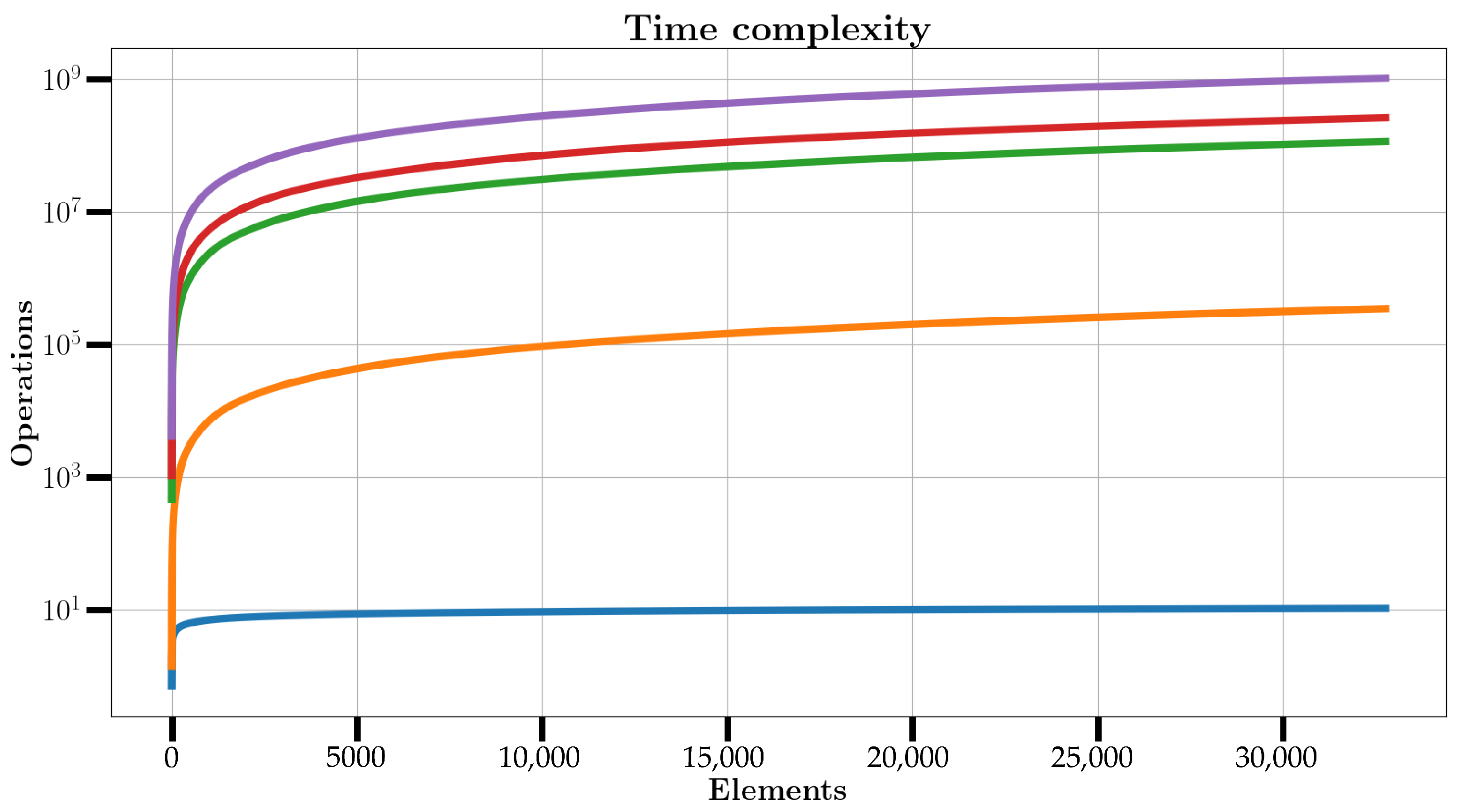
Figure 4 presents a graphical representation of the complexities: $log\left(n\right)$ is shown in blue, $nlog\left(n\right)$ is shown in orange, EMD complexity is shown in green, BEMD complexity using 4 projections is shown in red, and the purple curve shows the complexity using 16 projections. The complexities of EMD and BEMD have thus the same evolution than the FFT but with a larger multiplicative factor. However, the number of projections P in BEMD may considerably increase the calculation time.

Figure 4 presents a comparative analysis of the time complexity for several computational algorithms as a function of the number of elements processed. The plot employs a logarithmic scale on the y axis to effectively illustrate the growth rates of the operations required by each method. The blue curve represents logarithmic complexity denoted as log(n), which exhibits minimal growth even as the input size increases. This behavior is characteristic of highly efficient algorithms such as binary search, where the computational demand remains low regardless of the dataset size. The orange curve corresponds to linearithmic complexity expressed as n log(n), a pattern commonly observed in algorithms like the Fast Fourier Transform FFT. Although more computationally intensive than logarithmic complexity, its subquadratic growth ensures that it remains feasible for large datasets. The green curve depicts the complexity of the classic EMD algorithm. While EMD shares the same asymptotic growth as FFT, it involves a larger multiplicative factor, resulting in higher computational requirements for equivalent input sizes. The red and purple curves illustrate the complexity of the BEMD algorithm using 4 and 16 projections, respectively. BEMD extends the EMD approach by using multiple projections, which adds computational overhead. With 4 projections, as used in this research, the complexity remains comparable to EMD but diverges more significantly as the number of elements increases. When 16 projections are used, the computational demand rises substantially, as evidenced by the steeper ascent of the purple curve. This visualization highlights the scalability of algorithms with subquadratic growth, emphasizing their suitability for large-scale applications. It also underscores the trade-off in BEMD between accuracy, which improves slightly with more projections ([31]), and computational cost, which increases correspondingly. Although the constant factors of EMD and BEMD are larger than those of the FFT, their asymptotic complexity remains comparable, and BEMD offers a more expressive multicomponent decomposition that often warrants the additional processing effort.

4.3. Enhancements in the BEMD Implementation

Building upon our streamlined implementation from [5], we have integrated additional optimizations into the code. Specifically, we omitted symmetry extensions at the signal borders, which are conventionally used to mitigate edge effects and ensure accurate envelope calculations during the sifting process. Instead, our approach relies on capturing additional sampling points and truncating the boundaries, effectively avoiding cubic interpolation artifacts. This eliminates the need for symmetry extensions in real-world software-defined radio (SDR) applications.

Furthermore, the stopping criterion for the inner loop was modified, employing a fixed number of siftings instead of a Cauchy-type or Rilling’s improved stopping criterion [28]. This adjustment simplifies the process by reducing the number of sifting loops and thus leads to a notable reduction in the overall decomposition time. We also reduced the dataset precision from float64 to float32, yielding lower memory consumption and faster computation with no observable loss in classification accuracy.

Additionally, in the dataset aggregation process, we have opted for a more efficient approach. Instead of utilizing the modular (and algorithmically appealing) method of generating data slices and merging them, we now create a single large and empty tensor. Replacing each data slice individually helps mitigate the challenges posed by Python (version 3.14 at the time of writing) modules like NumPy, which tend to duplicate the entire dataset of tensors during decomposition, thus doubling the needed RAM memory. Moreover, we observed a phenomenon that we term adjacent trends (see Section 4.5). This effect can be mitigated by strengthening a constraint in the stopping criteria (see Section 4.4). Finally, when possible, we chose the Python tuples data type over the list data type, as tuples are immutable objects, consuming less memory and functioning as faster lookup tables.

Through the described optimizations, our decomposition approach not only reduces the discrepancy between training and validation accuracy, indicating a lower tendency to overfit, but also provides a significant time advantage in terms of decomposition time.

4.4. Stopping Criteria

When employing cubic interpolation in the extraction algorithm for the IMFs, an additional computational verification is required to ensure that the residual contains at least three extrema points. These extrema are essential for accurate interpolation and proper IMF decomposition. If the residual lacks sufficient extrema, indicating it closely resembles a linear trend, the decomposition algorithm is terminated.

The typical stopping criteria is

$$n_{min}+n_{max}\le 3$$

(4)

with $n_{min}$ being the number of detected minima points and $n_{max}$ being the number of maxima points.

On the contrary, when dealing with larger waveforms containing a greater number of samples, the decomposition generates an excess of IMFs.

This outcome is undesirable for AI classification because increasing the number of IMFs in the input results in a significant rise in initial weights at the CNN input layer. Consequently, the decomposition process in terms of time and memory, along with the subsequent training phase, may exceed the hardware capacity, especially on constrained systems.

Therefore, to avoid this issue without declining the information of the IMFs too much, a more constrained stopping criteria has been created:

$$n_{min}\le 3\mathrm{or}{n}_{max}\le 3$$

(5)

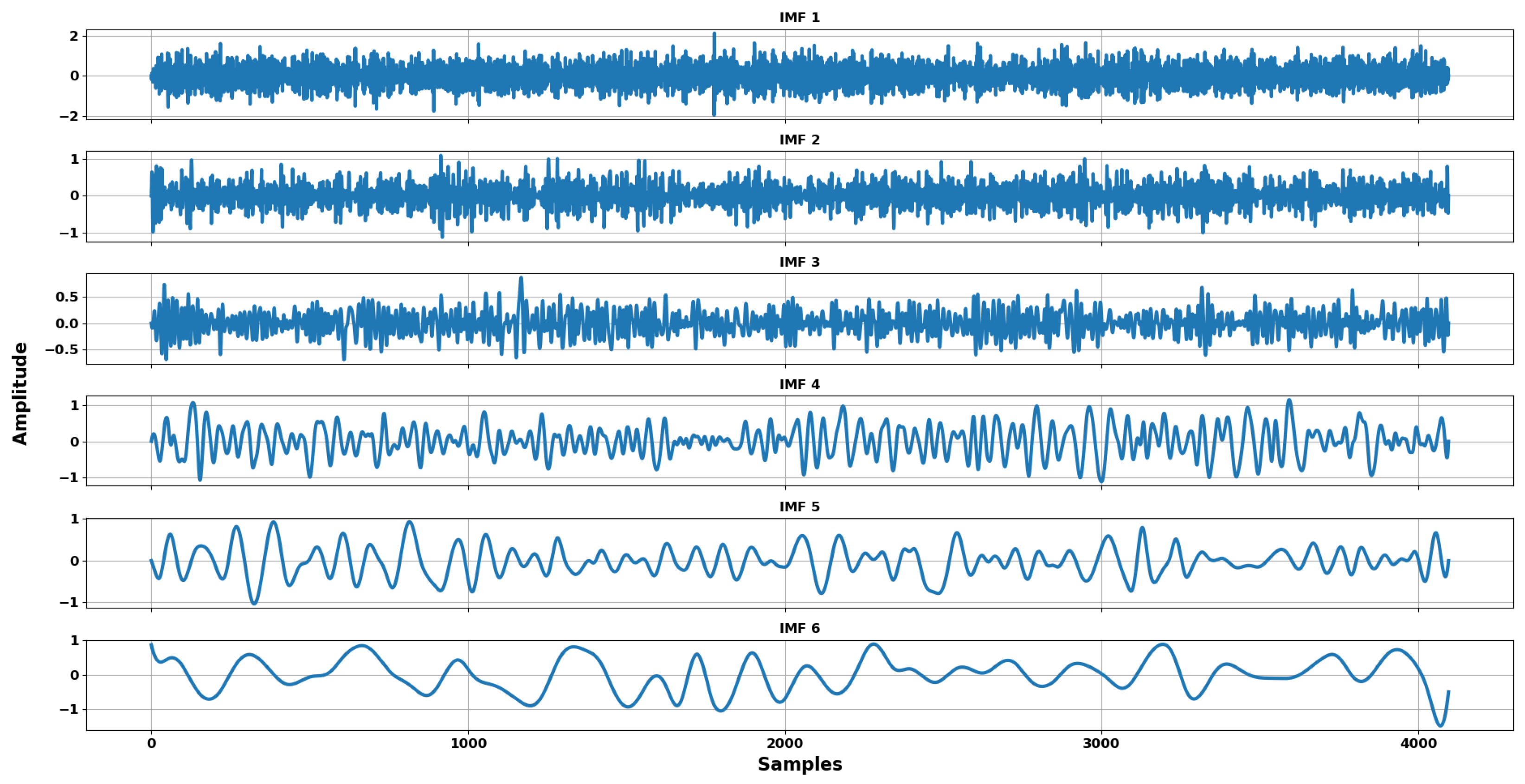
It provides a smaller, more manageable number of IMFs, enhances IMF quality, and has fewer adjacent trends (see Section 4.5). Figure 5 displays the six IMFs extracted from a DQPSK signal with an SNR of approximately 10 dB. As the IMF index increases, the number of oscillations decreases, illustrating the scale-separation property of the BEMD decomposition.

4.5. Limiting Adjacent or Secondary Trends

One characteristic commonly observed in empirical mode decomposition is the presence of a linear trend in the last intrinsic mode function, also called the residual. Upon applying the decomposition to datasets with higher sample counts, we observed that the last few IMFs often lack significant information or exhibit minimal oscillations. Typically, these IMFs manifest as subtle curves, closely resembling a straight line. This behavior is particularly pronounced in telecom IQ signals, which naturally oscillate around zero due to the inherent symmetry of IQ constellations. Consequently, the final trend or trends remain nearly flat, unlike in financial market data, where trends often show clear upward or downward drifts. We refer to these IMFs as adjacent or secondary trends.

The notion of adjacent trends is empirical, motivated by the observation that multiple low-energy IMFs with similar, minor fluctuations add little value to the CNN. Such components mainly introduce redundancy and can obscure more informative structures in higher-energy IMFs. As a possible criterion, one may classify as adjacent any IMF whose energy contribution falls below about 5% of the total signal energy and that shows no significant peaks or deviations. By adjusting the decomposition parameters, these low-energy IMFs can be merged into a single, more meaningful residual component. This preserves the essential information while reducing computational and memory costs, with a negligible impact on model performance.

Ideally, the goal is to obtain a decomposition in which the oscillatory behavior decreases in frequency with an increasing IMF order, and the residual reduces to a linear trend. With the improved code and stricter stopping criteria, we also mitigate the influence of adjacent trends. In our case, we extract approximately 10 to 20% fewer slightly curved intrinsic mode functions (IMFs) that lack relevant information and are unnecessary for the training of the AI architecture.

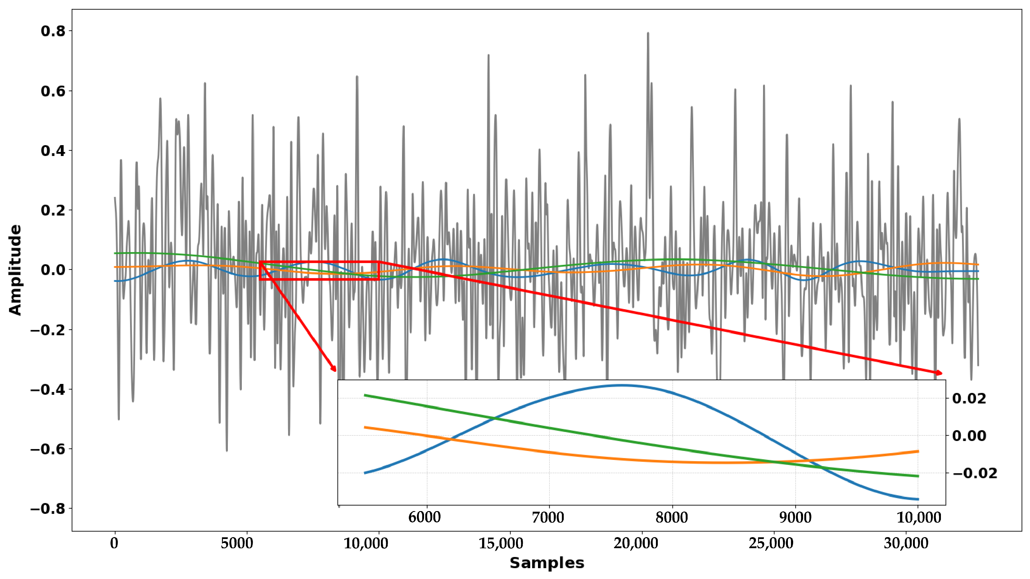
Similarly, fewer adjacent trends result in a reduced tensor size, leading to less data to store and fewer weights to train. This reduction translates into shorter training and decomposition times without compromising the integrity of the information. Figure 6 presents the real parts of the last three IMFs extracted using the original G. Rilling method [27], while the gray curve represents the last IMF obtained with our approach. It is evident that our method yields a component with higher energy and more pronounced oscillations in contrast to the original method, which mainly captures low-amplitude trends.

Examples of the number of extracted IMFs, as well as their corresponding energy levels depending on the modulation type and decomposition method, can be found on our GitHub [32].

4.6. Comparison of IMF Extraction Methods via Mean Percentage Vector (MPV)

To evaluate the efficiency of the proposed IMF extraction method, we compare both the number of extracted intrinsic mode functions (IMFs) and their energy distribution with those obtained from the baseline approach, Rilling’s method [27]. For each signal, IMFs are obtained using both methods, and the energy percentage of each IMF relative to the original signal is computed. The Mean Percentage Vector (MPV) is derived by averaging these energy percentages across all signals.

Let N denote the number of signals in the dataset, and let $M_i$ represent the number of IMFs extracted for the i-th signal. The energy percentage of the j-th IMF for the i-th signal is denoted as ${\mathrm{perc}}_{i,j}$. The MPV is then calculated as

$${\mathrm{MPV}}_j={\displaystyle \frac{1}{N}}\sum _{i=1}^N{\mathrm{perc}}_{i,j}$$

where ${\mathrm{MPV}}_j$ is the mean energy percentage of the j-th IMF across all signals. This metric provides a concise representation of the typical energy distribution of IMFs in the dataset. As shown in

Table 3. Comparison of IMF Extraction Methods.

Method	Decomposition Time (s)	Number of IMFs	MPV (%)
Rilling	4.73	5 IMFs: 2 6 IMFs: 34 7 IMFs: 4	IMF 1: 26.22 IMF 2: 14.29 IMF 3: 11.78 IMF 4: 16.13 IMF 5: 13.40 IMF 6: 16.17
Proposed (Cubic)	1.15	4 IMFs: 1 5 IMFs: 36 6 IMFs: 3	IMF 1: 28.55 IMF 2: 15.89 IMF 3: 17.59 IMF 4: 26.77 IMF 5: 34.63 IMF 6: 4.00

, the improved method extracts fewer IMFs on average yet concentrates a greater proportion of the signal’s energy in the initial components. This indicates that the improved method achieves a more compact and informative decomposition, capturing the dominant modes more effectively. As a note, the Mean Percentage Vector (MPV) represents the average energy contribution of each IMF across all signals in the dataset. Because individual signals may decompose into different numbers of IMFs, the sum of the MPV values can exceed 100 percent. This is expected and indicates the average distribution of energy across signals, not the total energy of a single signal. It is a valid metric for comparing decomposition methods.

5. Results and Discussion

The computations presented in this study were performed on the Dragon2 High Performance Computing (HPC) cluster. Hosted by the University of Mons (UMONS) and integrated into the Consortium des Équipements de Calcul Intensif (CÉCI) [33], Dragon2 is optimized for long running and resource-intensive simulations and data processing. The cluster features 17 compute nodes, each equipped with dual Intel Skylake 16 core Xeon 6142 processors operating at 2.6 GHz. Most nodes provide 192 GB of RAM and two nodes offer 384 GB of RAM. In addition, two GPU accelerated nodes, each fitted with two NVIDIA Tesla V100 GPUs, enable parallel and accelerated computing. Communication between nodes is supported by a 10 Gigabit Ethernet interconnect, and the Slurm job scheduler allows a maximum job duration of 21 days, which is suitable for extended simulations and data processing tasks.

Although the Dragon2 cluster provides substantial computational resources, multiprocessing of the BEMD algorithm remains difficult because the algorithm is inherently iterative and recurrent. For this reason, multiprocessing was not used in this work. In addition, all computations, including CNN training and BEMD processing, were performed on CPU nodes without the use of GPU acceleration in order to maintain a constrained and reproducible software environment. The effective performance of these nodes is comparable to that of a standard commercial laptop equipped with an Intel Skylake processor operating at 2.60 GHz and a maximum of 24 GB of RAM. Working under these controlled conditions ensured that all experiments could be repeated reliably and that model training was performed under identical computational settings.

At the current stage, BEMD is not suitable for real-time AMC applications because of its recursive and iterative structure. Even though the processing time of the algorithm has been reduced compared with earlier work, it is not expected to reach real-time performance, especially at higher sampling rates. BEMD remains a viable approach for offline analysis of sensitive or high-quality recorded data where computational latency is less critical. In contrast, the SSA concept can be implemented using alternative algorithms that meet real time constraints. Although the complete pipeline has not yet been deployed on embedded hardware, such implementations are feasible and are part of ongoing research.

The AI module for this study is implemented using TensorFlow, leveraging its powerful tools for deep learning. The training process is constrained to a maximum of 100 h, with an early stopping mechanism integrated to optimize computational efficiency. The early stopping mechanism employs a patience parameter of 10, halting training if no improvement in accuracy or loss function is observed over 10 consecutive epochs.

As previously mentioned, the architecture is based on convolutional neural networks, which are feed-forward neural networks. The core of CNNs lies in their convolutional layers, which convolve feature maps from previous layers using trainable kernels or filters. In this implementation, the convolutional layers are complemented by fully connected (dense) layers, functioning as Multilayer Perceptrons (MLPs) that are directly connected to the preceding layers.

Key elements of the architecture include ReLU (Rectified Linear Unit) activation functions, dropout layers to prevent overfitting, and flattening operations to transition between CNN and dense layers. Notably, pooling layers are omitted due to the small height of the input data and the need to retain all critical information, avoiding the potential loss associated with averaging operations [24].

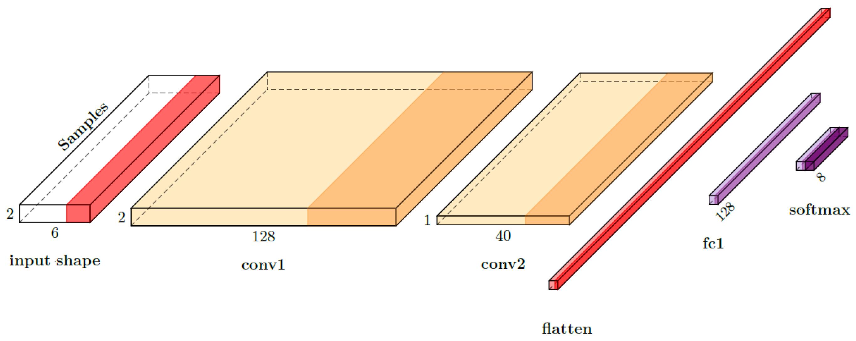
The specific configuration begins with a convolutional layer (conv1) comprising 128 filters of size 1 × 3, followed by a second convolutional layer (conv2) with 40 filters of size 2 × 3. The final dense layer, sized at 8 to correspond to the number of possible modulation classes, incorporates a softmax activation function to produce the output probability distribution. This architecture uses only half the number of parameters compared to the model presented in [5] and is derived from the structure proposed in [9]. The model preserves the same proportional ratio of nodes as in the original architectures but employs fewer absolute nodes because our input representations contain significantly more samples than those in O’Shea’s dataset. This design choice allows us to control computational cost while maintaining performance.

This configuration is illustrated in Figure 7 and detailed in

Table 4. CNN Architecture Summary.

Layer Type	Kernel/Units	Activation
Input	(batch size, 2, samples, 6)	–
Conv2D	(1, 3), 128	ReLU
Dropout	50%	-
Conv2D	(2, 3), 40	ReLU
Dropout	50%	-
Flatten	–	–
Dense	128	ReLU
Dropout	50%	-
Dense (output)	8	Softmax

. The CNN architectures were designed using PlotNeuralNet [34] for visual clarity and documentation.

Using the original O’Shea dataset, the baseline model employing IQ samples and a CNN across all SNR values and modulation types achieves an overall classification accuracy of 51.8%. When applying the cubic spline method with fixed sifting iterations of three and four projections, eight IMFs (compared to six in this study), and a waveform length of 128 samples (the maximum in that dataset), the accuracy improves to 53.86%, representing an increase of around 2.1% in overall classification accuracy. The improvement is more pronounced at higher SNR values, reaching 4.4% at 12 dB.

In earlier work based on O’Shea’s 128-sample dataset, the maximum number of IMFs obtainable using Rilling’s improved stopping criterion (see Ref. [28] with threshold1 = 0.05, threshold2 = 0.5, $\alpha =0.05$) was eight, which was adopted as the baseline; signals yielding fewer IMFs were zero-padded accordingly. In the newer CSPB.ML.2018 dataset, the substantially longer waveforms allow for the extraction of up to approximately 20 IMFs. To preserve consistent input dimensions and maintain feasible memory requirements for sequences of up to 32,000 samples, the architecture in this study is therefore restricted to six IMFs. This number is therefore not an inherent optimal value, but rather the result of limits imposed by memory constraints and maximum input size. No convergence instabilities attributable to the decomposition depth were observed, although a dedicated analysis was not performed. This aspect may further depend on the specific CNN configuration (e.g., conventional vs. separable convolutions) and remains a subject of ongoing investigation. In this work, classical 2D CNN layers have been used.

In

Table 5. Classification results in overall validation accuracy (%).

Data-Length (Samples)	Original IQ	SSA BEMD IQ
128	50.4	54.2
256	56.5	58.4
512	62.2	70.0
1024	58.2	73.0
2048	65.2	76.5
4096	46.6	77.4
8192	46.8	76.2
16,384	47.2	70.6
32,768	47.0	75.2

, the results, except for the last three rows, are obtained via the mean validation accuracy of a 10 K-fold training setup. The last three rows, however, are averaged over three or fewer independent training sessions, as model convergence for these long data sequences is particularly challenging, especially given the limited capacity of the small AI model used. It is worth noting that the classical IQ method saturates at around 45% accuracy, while the absence of convergence in our setup would yield a baseline accuracy of 12.5% (random chance for eight possible modulation classes), which are always rejected and not taken into account in averaging. Despite these challenges, our method demonstrates improved classification performance on the validation data as well as a higher likelihood of convergence. To ensure consistency with the baseline method, only 50% of the data was allocated for training, with the remaining 50% reserved for validation.

The impact of data length on classification performance, as shown in Table 5, provides key insights for our CNN architecture of fixed size. When the decomposed signal is used as input, validation accuracy consistently surpasses that of the original IQ signal for all sample lengths. The original IQ input shows a clear saturation point, with accuracy peaking at 65.2 percent for 2048 samples before declining for longer sequences. Conversely, the BEMD-SSA combination delivers a minimum absolute accuracy improvement of 20 percent and sustains strong performance even as sample length increases, achieving a peak of 75.2 percent at 32,768 samples. This indicates that the decomposed representation effectively addresses the performance degradation observed with longer inputs when raw IQ data is used. However, we observe that convergence becomes progressively more challenging as the waveform length increases. An important consideration is the computational cost associated with increasing sample length. For our network, doubling the number of samples has a much larger impact on model size and resource demands than doubling the number of input channels, such as IMFs. While increasing channels mainly influences the first convolutional layer by expanding kernel depth and the number of learnable parameters per filter, longer samples extend the input feature map across all layers. This affects every convolutional operation, leading to a higher memory footprint and computational load throughout the entire CNN pipeline, given the fixed kernel size and filter count. Thus, the decomposed input not only improves accuracy but also presents a more efficient approach for handling longer sequences within our architecture constraints.

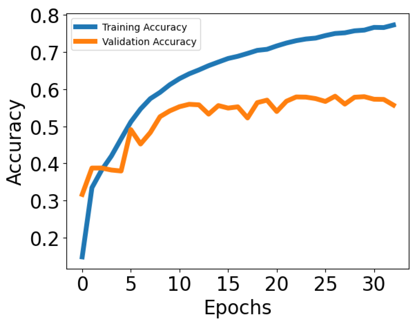
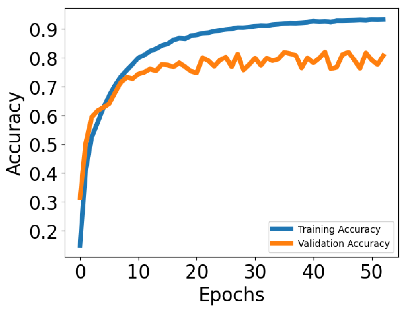
Figure 8 and Figure 9 illustrate the training and validation accuracy for the classical IQ approach and our BEMD approach, respectively. Training accuracy quantifies the model performance on the samples used during optimization, while validation accuracy evaluates the performance on separate unseen samples and therefore indicates the model’s ability to generalize. Notably, our method exhibits a significantly smaller gap between training and validation accuracy, indicating reduced overfitting. Additionally, the validation accuracy is higher and converges more rapidly compared to the classical approach.

6. Conclusions

This work demonstrates that signal surface augmentation combined with Bivariate Empirical Mode Decomposition provides a significant improvement in automatic modulation recognition by expanding the effective data surface presented to convolutional neural networks. The proposed enhancements to the BEMD process, namely optimized stopping criteria, reduced adjacent trends, and improved memory handling, yield more informative decompositions and consistently higher classification accuracy across all waveform lengths tested, including long sequences.

However, the approach also presents certain constraints. Despite the implemented optimizations, BEMD remains computationally demanding and is not yet suitable for real-time AMC operation. In addition, all evaluations were performed on synthetic datasets that, while realistic, do not fully capture the variability of real RF environments, and the fixed number of extracted IMFs was limited by memory considerations rather than by an intrinsic optimum. The lightweight CNN architecture used here provides a fair comparison between IQ and SSA-based inputs but does not exploit the full potential of more advanced deep learning models.

Overall, the results confirm that SSA is a promising and scalable preprocessing strategy that can substantially improve the robustness of modulation recognition. Future work will focus on accelerating SSA-compatible decompositions, validating the method on real measured signals, and exploring alternative multi-scale representations to further broaden its applicability in modern communication systems.