Article

Beyond “One-Size-Fits-All”: Estimating Driver Attention with Physiological Clustering and LSTM Models

by
Juan Camilo Peña
1,
Evelyn Vásquez
1,
Guiselle A. Feo-Cediel
1,
Alanis Negroni
2 and
Juan Felipe Medina-Lee
2,*
1
Department of Electrical and Computer Engineering, Faculty of Engineering, University of Puerto Rico, Mayaguez Campus, Mayaguez, PR 00680, USA
2
Department of Computer Science and Engineering, Faculty of Engineering, University of Puerto Rico, Mayaguez Campus, Mayaguez, PR 00680, USA
*
Author to whom correspondence should be addressed.
Electronics 2025, 14(23), 4655; https://doi.org/10.3390/electronics14234655
Submission received: 9 September 2025 / Revised: 20 October 2025 / Accepted: 22 October 2025 / Published: 26 November 2025
(This article belongs to the Special Issue Wearable Sensors for Human Position, Attitude and Motion Tracking)

Abstract

In the dynamic and complex environment of highly automated vehicles, ensuring driver safety is the most critical task. While automation promises to reduce human error, the driver’s role is shifting to that of a teammate who must remain vigilant and ready to intervene, making it essential to monitor their attention level. However, a significant challenge in this domain is the considerable inter-individual variability in how people physiologically respond to cognitive states, such as distraction. This study addresses this by developing a methodology that first groups drivers into distinct physiology-based clusters before training a predictive model. The study was conducted in a high-fidelity driving simulator, where multimodal data streams, including heart rate variability and electrodermal activity, were collected from 30 participants during conditional-automated driving experiments. Using a time-series k-means clustering algorithm, the researchers successfully partitioned the drivers into clusters based on their physiological and behavioral patterns, which did not correlate with demographic factors. Then, a Long Short-Term Memory model was trained for each cluster, which achieved similar predictive performance compared to a single, generalized model. This finding demonstrates that a personalized, cluster-based approach is feasible for physiology-based driver monitoring, providing a robust and replicable solution for developing accurate and reliable attention estimation systems.

1. Introduction

Safety in autonomous driving scenarios has become a constantly growing field of research in recent years [1,2], reflecting a growing interest in understanding the human factors that influence this activity. An important element is the reaction time of the drivers, which largely depends on maintaining an adequate level of attention [1,3,4,5]. This relationship between attention and reaction time is particularly relevant in situations where drivers temporarily divert their attention from driving [6], since a reduction in attention increases response time and increases the risk of incidents when regaining control of the vehicle [6,7], making it essential to have methods that allow monitoring and anticipating the driver’s attention level [1,7,8,9].
Methods proposed in the literature for determining attention levels still pose key challenges. Image-based approaches struggle to interpret data when dynamic conditions, such as weather, lighting, or ambient motion, are present. In contrast, physiological data allow direct assessment of the driver’s internal state without relying on external factors. However, these types of signals present high individual variability [1,9,10,11], since the human body’s reactions to mental stress are highly subjective and depend on the characteristics of each person [8,9]. This variability makes it challenging to build universal models and raises the need for approaches capable of handling such heterogeneity.

1.1. Similar Studies

The use of recurrent neural networks, particularly Long Short-Term Memory (LSTM), has established itself as a robust method for analyzing and predicting time series in driver monitoring. Several studies have used LSTM-based models to estimate driver states such as distraction or attentional engagement from physiological data [12]. For example, ref. [13] evaluated distraction and drowsiness in a simulator with 45 participants, using pulse blood volume, breathing, conductance, and cutaneous temperature signals. They compared traditional classifiers with an LSTM network and found that deep spacetime representations outperformed classical methods. Likewise, ref. [14] proposed an architecture with attention and Bidirectional LSTM (BILSTM) to predict performance in takeover situations during automated driving; this approach, which integrated indicators of the driver’s state, the traffic environment, and personal attributes, surpassed other comparative algorithms, showing the effectiveness of explicitly modeling the temporal dependence on these predictions. However, these works demonstrate the potential of LSTM-based architectures, but they generally train a single model on grouped data from all participants, implicitly assuming homogeneity across subjects.
Physiological sensing in driving and related human–machine interaction scenarios increasingly relies on sequential models to capture the dynamics of the subject’s electrocardiogram (ECG) and electrodermal activity (EDA). LSTM architectures are a natural fit for these data due to their ability to model long-range temporal dependencies and nonstationarity in autonomic responses. Recent studies show that Bayesian optimization can efficiently tune LSTM hyperparameters and thereby improve accuracy and robustness on physiological tasks; for example, Bayesian optimization has been used to adjust BILSTM learning rates and hidden sizes for ECG classification, and to optimize LSTM-based lead transformation models intended for wearable or reduced-lead settings [15,16]. Bayesian optimization has also proven valuable in other fields beyond biosignals, where spatiotemporal LSTM variants optimized by BO have advanced driver-state and control prediction problems such as steering-angle estimation, further underscoring the interplay between sequence models and sample-efficient hyperparameter search [17].
There are reported studies that have emphasized not only the usefulness of physiological data, but also their substantial variability between subjects, as individuals may react differently to the same stimulus [1,9,10,11]. In the context of driving, ref. [1] developed a multisensor system that simultaneously recorded EEG, ECG, and EDA-SPR signals during manual and autonomous driving scenarios in a simulator device. From these signals, they extracted blink frequency and beta-band power from EEG, heart rate from ECG, and RMS measures from EDA-SPR. Their results showed that manual driving elicited greater attentional engagement than autonomous driving, demonstrating that these physiological indicators reliably reflect the driver’s perceived level of attention. In addition to physiological signals, behavioral indicators such as the hands on wheel (HOW) can be a valuable indicator of the driver’s level of attention and willingness to regain control of the vehicle [18,19]. Research on partial collaborative systems has shown that keeping hands on the wheel improves monitoring behavior and recovery performance during automated command transitions [19].
In other application domains, hybrid approaches combining clustering techniques with LSTMs have been explored to improve model efficiency and accuracy. For example, in ref. [20], k-means clustering was applied to air quality time series to predict the average daily concentration of particles with a diameter less than 10 μ m in Malaysia, reducing the number of models and the total training time. Similarly, ref. [21] proposed a scheme based on time-series clustering and sequence-to-sequence LSTM models for forecasting electrical load in homes, achieving notable improvements in efficiency and accuracy.

1.1.1. Research Gap and Contributions

While recent advanced data-driven methods have shown promising results in processing complex physiological time series for driver-state estimation, a challenge persists: inter-individual variability in physiological responses to cognitive states. Drivers exhibit unique patterns in their heart rate, electrodermal activity, and other physiological signals even under similar levels of distraction or vigilance. Most deep-learning-based studies train these models on aggregated data from diverse participants, often overlooking explicit segmentation or adaptation to individual differences. This typically results in either per-person model training (which is sometimes impractical due to a lack of enough data and cold-start problems [22]) or reliance on demographic factors that may not truly capture underlying psychophysiological similarities. Consequently, a significant gap remains in developing scalable, effective methodologies that explicitly account for inherent physiological differences among drivers to group them. This approach would enable the training of more specialized, accurate predictive models. Specifically, the literature lacks a comprehensive strategy that systematically integrates physiological time-series clustering as a preliminary, adaptive step before training deep learning models for personalized, precise attention level prediction in autonomous driving contexts.
The main contribution of this study is the introduction of a novel methodology that systematically groups drivers into different clusters based on their physiological and behavioral time-series patterns, moving beyond generic or demographically driven classifications. By aggregating data from multiple individuals who exhibit similar underlying psychophysiological response patterns, the trained models can learn more generalizable and robust representations of attention within each cluster. This approach mitigates data scarcity for any individual, reduces the computational burden of managing countless unique models, and provides a scalable solution for adding new drivers by assigning them to an appropriate pre-trained cluster. Furthermore, we empirically discuss the capabilities of customized models applied to the identified physiological clusters, representing a notable advancement over conventional global models. This work provides practical evidence that intrinsic physiological patterns, rather than broad demographic factors, are more relevant for determining how individuals exhibit and process varying levels of attention, offering insight for the design of adaptive and personalized driver-monitoring systems.

1.1.2. Approach

Our approach integrates two key steps: (i) using a time-series k-means algorithm to group participants according to their unique physiological and behavioral patterns; and (ii) training cluster-specific LSTM models to capture more representative dynamics of attention. This alternative methodology, which uses signals such as ECG, EDA, and hands-on-wheel data as features, effectively complements global and personalized approaches by providing a practical, replicable solution that accounts for inter-individual variability. To evaluate the strategy’s effectiveness, its performance was compared with three alternative scenarios: a global model trained on all participants, models trained on principal component analysis (PCA)-based clusters, and models trained on clusters defined by demographic characteristics.

1.1.3. Research Questions and Hypotheses

Having analyzed the methods used for monitoring a driver’s attention level, it was observed that the grouping of physiological signals has rarely been considered a preparatory step for predictive attention models. Therefore, this study is based on the following research questions:
  • R1: Does clustering of physiological time series using time-series k-means offer an advantage in predicting the level of attention compared to global or random clustering?
  • R2: Can it be shown that membership in the obtained clusters does not directly depend on demographic variables such as age, gender, or years of experience, but instead on the observed physiological and behavioral dynamics?
To answer these questions, this study proposes an experimental design in which physiological signals (ECG and EDA) are collected, a clustering scheme is employed, and cluster-specific LSTM models are trained. The results are then compared against two reference conditions: (i) a global model trained on all participants and (ii) models trained on randomly generated clusters.
Consequently, this study investigates the following hypotheses:
  • H1: Cluster-specialized models, defined using time-series k-means, achieve higher predictive performance than global models and models trained with random clustering.
  • H2: Participant assignment to clusters is not explained by demographic characteristics, but by physiological and behavioral patterns.
The structure of this work is organized as follows: Section 2 describes in detail the implemented methods used in this study, including a description of the driving simulation experimental environment and the different scenarios designed, as well as the structure of the testing protocol, the technologies and equipment used, and the characterization of the participants. Next, Section 3 details the preprocessing methodology, which covers the initial data processing, the preprocessing of physiological characteristics, attention levels, and the hands-on-wheel metric, as well as the application of time-series k-means clustering, the design of the LSTM architecture, and Bayesian hyperparameter optimization. The results are presented in Section 4, including the findings from the clustering process, Bayesian optimization, and LSTM models. Subsequently, Section 5 discusses the performance of the LSTM models and the identified clusters. Finally, Section 6 summarizes the main findings and proposes future directions to strengthen the applicability of physiology-based clustering in real-life driving scenarios.

2. Methodology

The experimental study was conducted in a controlled driving simulation environment that allowed the incorporation of various scenarios, enabling engagement with different automated modes and attention levels. The aim was to simulate realistic urban and semi-urban driving scenarios with sudden events that required the driver to regain control, while systematically capturing multimodal data to assess reaction time, distraction level, and behavioral performance.
Throughout the test sessions, a structured experimental protocol was applied to a group of 30 participants, with their physiological signals and attentional states continuously recorded as they engaged in various driving situations. During the experiment, unexpected events were introduced to trigger takeover requests (TORs), including unsafe pedestrian crossings, traffic-impeding vehicles, and the sudden appearance of lane-blocking obstacles, enabling real-time evaluation of drivers’ reactions and physiological responses. To capture individual variability, the collected physiological data were used to generate participant clusters through unsupervised learning techniques. Based on these clusters, two machine learning training strategies were implemented and compared: (i) a global model, trained on the entire dataset as if the population were homogeneous, and (ii) segmented models, trained independently for each cluster.
Subsequently, the clusters were analyzed based on similarities in physiological parameter patterns to identify distinct behavioral trends and improve the interpretability of driver responses. Finally, the performance of both modeling strategies was compared based on their classification accuracy and their ability to adapt to the participants’ physiological diversity.
The remainder of this section outlines the test protocol’s structure, the experimental setup, the technologies and equipment employed, the data collected, and the characteristics of the participant group involved in the study.

2.1. Structure of the Test Protocol

To guarantee the quality and integrity of the physiological and attentional data collected during simulated driving tests, a structured experimental protocol was implemented. A total of N S = 30 participants were subjected to this procedure, which was organized into four distinct phases, as shown in Figure 1.
In the first phase, the functionality and connectivity of all critical systems were verified. This includes the devices listed in Section 2.2, which are responsible for data acquisition and logging.
The second phase focused on introducing the participants to the experiments. Individuals were presented with the informed consent form and received detailed instructions regarding the experiment. After consent was granted, the research team proceeded with the calibration and placement of physiological sensors.
The fourth phase of the protocol was dedicated to executing the main experiment. This phase begins with 5 min of rest to establish baseline data for each subject, followed by a 5 min experimental stage of manual driving practice in the environment. The primary objective of this practice is to allow participants to familiarize themselves with the sensitivity of the simulator’s controls—brake, accelerator, and steering wheel—and to understand the interaction with the human–machine interface.
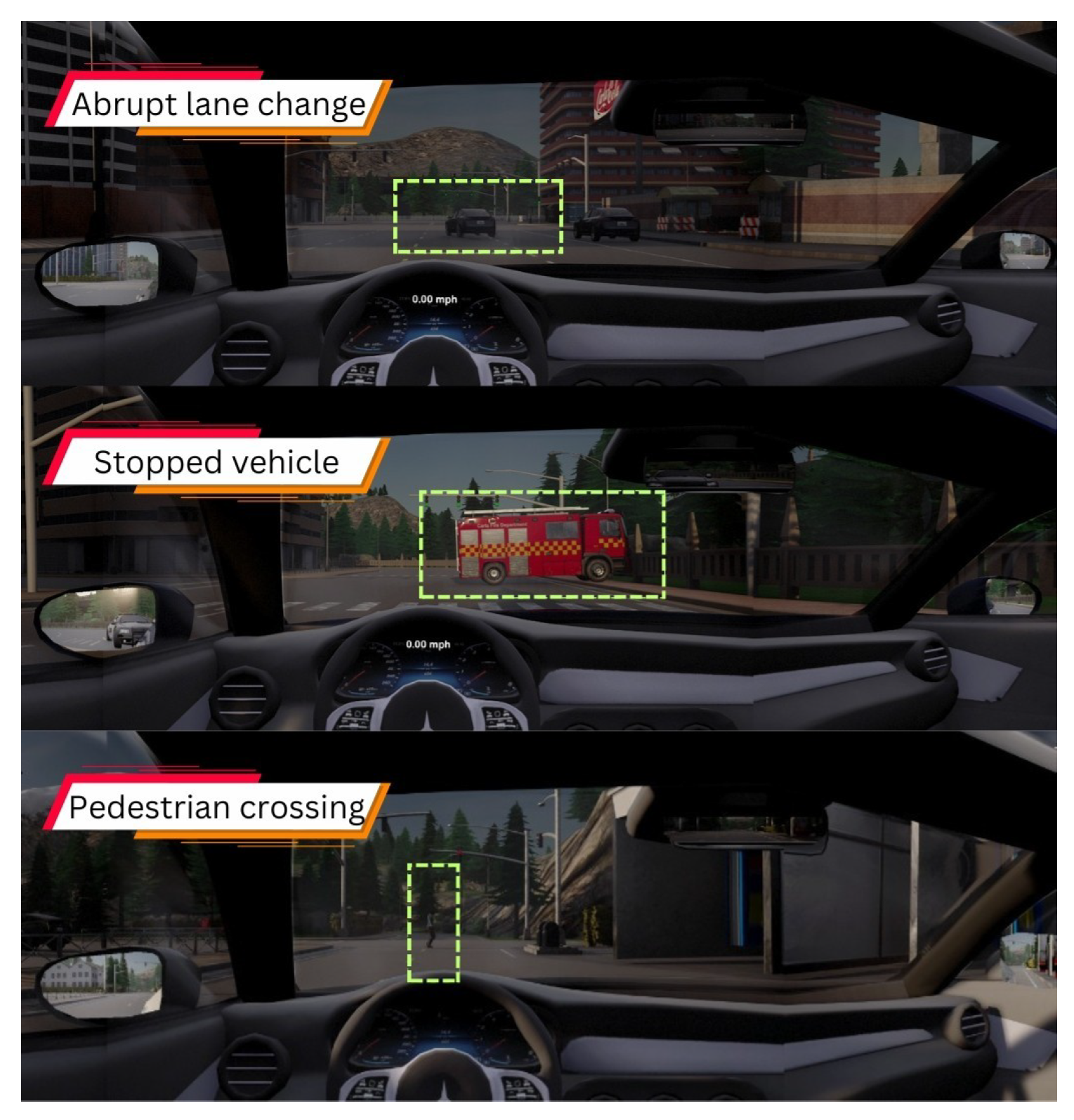
Following this familiarization period, participants undertook experimental tests to perform takeover requests during autonomous driving segments. When a takeover maneuver was required, an audible and visible alert on a tablet positioned next to the steering wheel prompted the participant to assume control. Once the critical situation was avoided, the human had to return the vehicle to autonomous driving mode. The experiments are comprehensively detailed in Table 1, which summarizes the experimental setup used in the study and provides an overview of the key characteristics of each evaluated scenario. The experiments were conducted on two different maps in the CARLA (Car Learning to Act) version 0.9.15 simulator to analyze participant behavior under increasingly complex conditions. The table includes information on the urgency levels of TORs (low, medium, and critical) and the concentration levels evaluated for each. The scenarios included sudden lane changes, pedestrian crossings, road obstructions, traffic accidents, and dynamic moving obstacles, designed to induce varying degrees of cognitive load and attention demands. Some of these scenarios are illustrated in Figure 2. The hazardous objects in the scenes are highlighted with green boxes: a sudden lane change, a fire truck in the middle of the road, and a sudden pedestrian crossing. Additionally, the table provides the approximate time of each TOR activation and the total duration of each experimental session, offering a comprehensive overview of the test design, sequence, and complexity.
To systematically evaluate the participants’ attention levels during driving experiments, a dual-task experimental paradigm was implemented, combining the primary driving simulation with secondary tasks. To induce varying levels of cognitive load, participants interacted with a mobile word search application at predefined stages of the experiment. This task simulated realistic driver distraction and provided a richer dataset for characterizing fluctuations in attention levels, complementing the primary performance metrics collected.
In parallel, a visual attention assessment was integrated into the driving environment. Geometric figures—circles, squares, triangles, and stars—were projected onto the side screens in distinct colors (red, green, blue, yellow, violet, and cyan) at 20 s intervals, each displayed for 2.5 s. Participants were instructed to respond by manipulating a switch lever to indicate whether the star stimulus appeared on the upper (Figure 3a) or lower region (Figure 3b) of the respective screen. This action evaluated their level of attention and generated a detailed record in the Attention Logs, which will be described in Section 3.4. This procedure allowed for continuous, time-resolved assessment of visual detection performance and attentional engagement. Similar approaches have been successfully applied in driver workload studies, where secondary visual tasks combined with psychophysiological markers provide reliable indicators of attention allocation and cognitive state [23].
Additionally, takeover requests were introduced to evaluate participants’ readiness to regain control during automation disengagement events. TORs were triggered seven seconds before a critical scenario, communicated via a tablet-based human–machine interface (HMI). Participants were required to press the “Take Control” button on the touchscreen to manually navigate around the obstacle and subsequently reactivate autonomous mode after clearing the hazard. These TOR events, combined with concurrent visual and mobile tasks, generated a multimodal dataset that linked attentional performance and physiological indicators.

2.2. Technologies and Equipment Used

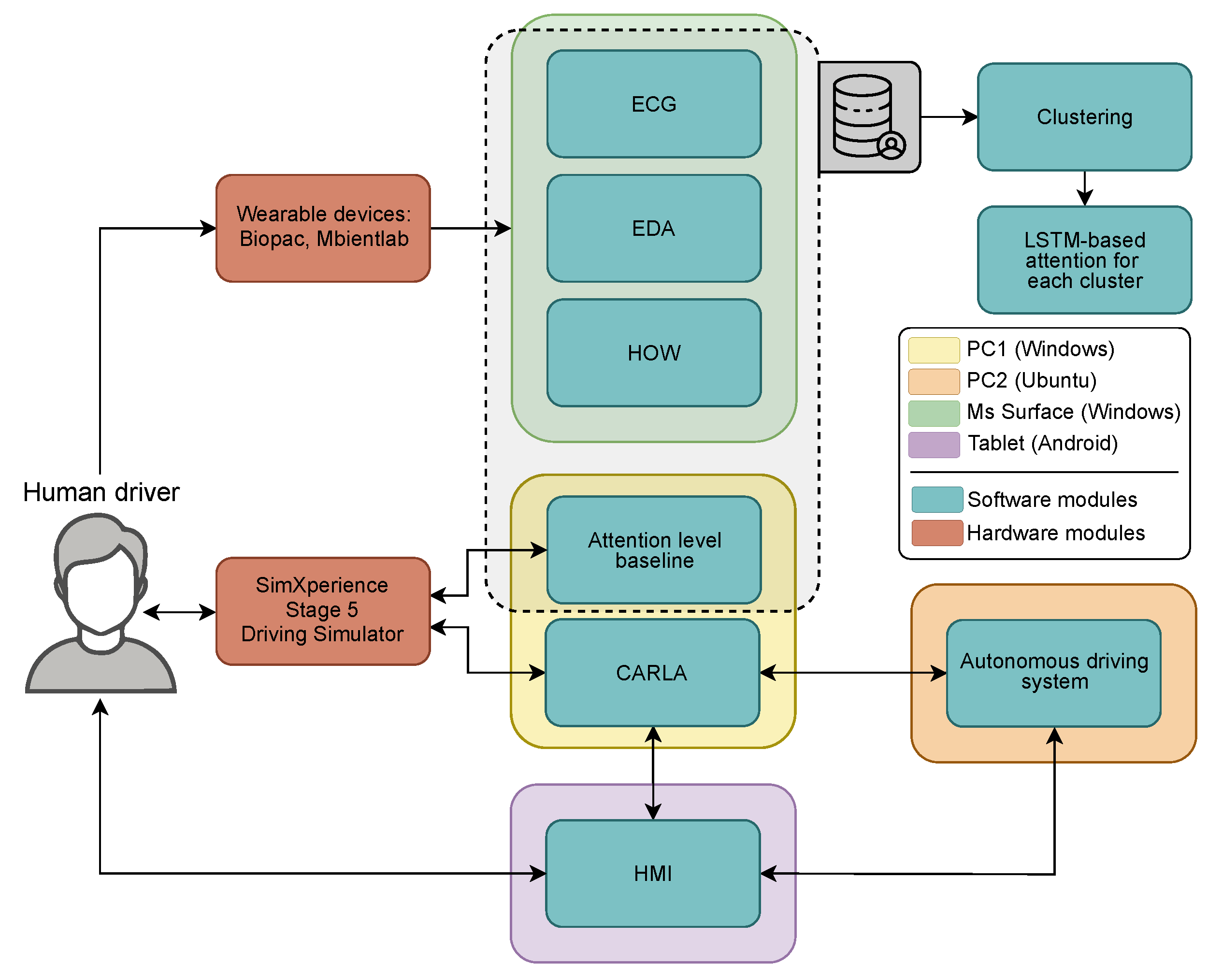
This section describes the complete experimental setup used in this work, integrating software, wearable sensors, and computational systems. Figure 4 provides an overview of the entire architecture, illustrating the interaction between simulation tools, physiological monitoring devices, and computing platforms, and summarizes the multi-stage experimental framework designed to capture the complexity of the interaction between humans and vehicles in autonomous driving. Each module, from vehicle control to physiological detection, was developed to interact systematically, enabling analysis of the user’s attention dynamics and interaction with the experiment.
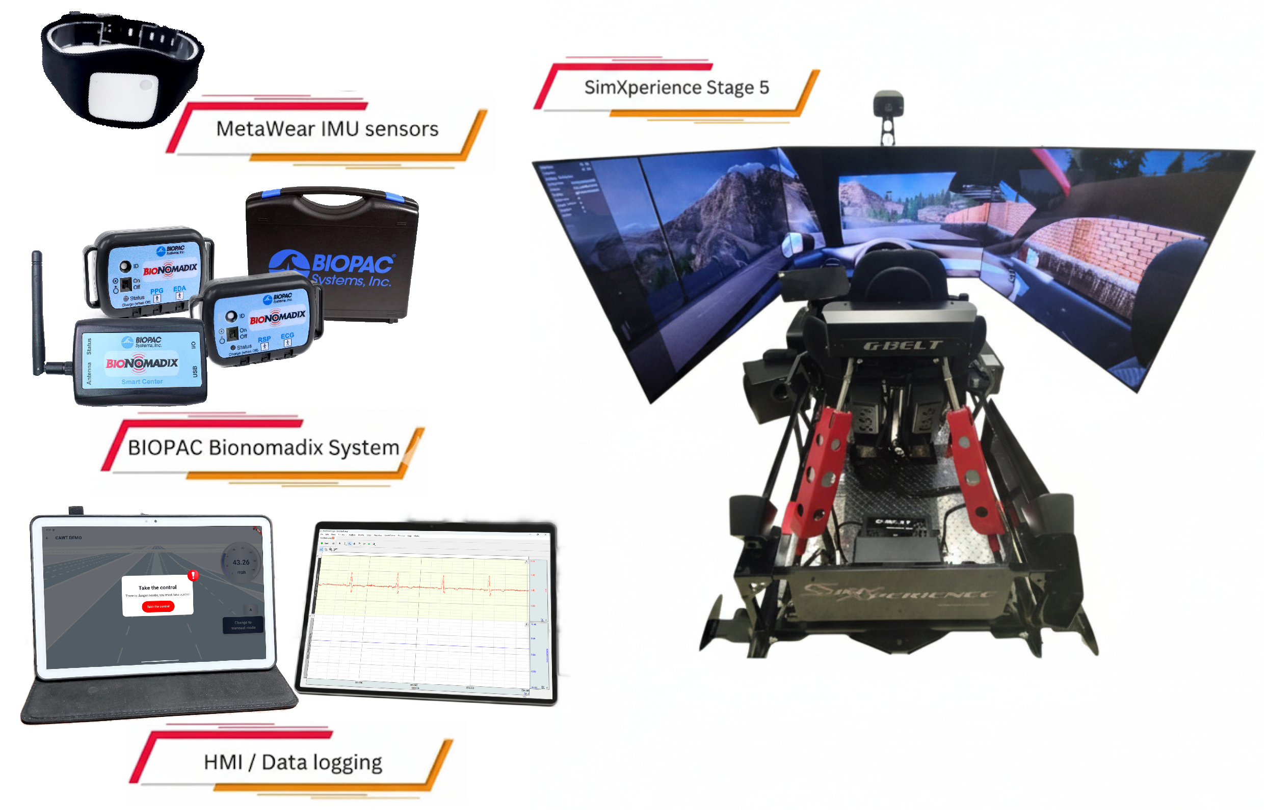
The experiments were conducted using the SimXperience Stage 5 simulation platform (SimXperience, Akron, OH, USA), which incorporates a multi-axis motion system, surround sound, and feedback from the steering wheel and seat. This setup aims to increase drivers’ immersion in the physical sensations of real-life driving, allowing them to experience acceleration, braking, and cornering with high fidelity. Using an environment with these characteristics is essential for ensuring that the physiological responses recorded in the ECG and EDA accurately reflect driving conditions similar to those in a real-life environment [24,25]. Figure 5 illustrates the whole experimental setup, including the driving simulator, the human–machine interface for control interaction, the MetaWear IMU sensors for motion tracking, and the Biopac Bionomadix system (BIOPAC Systems, Inc., Goleta, CA, USA) for physiological signal acquisition (a demonstration video of the system is available at https://www.youtube.com/watch?v=Xa7oBMYvrkg (accessed on 19 October 2025).). This integrated platform enabled synchronized collection of multimodal data streams necessary for evaluating driver behavior and physiological responses under semi-automated driving conditions.
The experiments were conducted in CARLA, an open-source simulator designed to support the development, training, and validation of autonomous systems in highly configurable virtual environments. CARLA is powered by the Unreal Engine 4.26.2 graphics engine, which enables high-fidelity rendering and realistic physics. It supports a wide range of sensor modalities (e.g., cameras, LiDAR, IMU, GPS) and environmental conditions (e.g., lighting, weather), making it a widely adopted tool in the autonomous vehicle research community. More details about CARLA and its documentation can be found in [26].
The experimental environment was built using CARLA towns 4 and 5, which provide diverse urban and semi-urban settings. These maps were digitized in the lanelet2 format [27], allowing the autonomous driving system to navigate them with precise definitions of lane geometries, regulatory elements, and routing logic.
While the combination of the SimXperience Stage 5 motion platform and the CARLA simulator provides a high-fidelity, immersive, and highly controllable environment, essential for the safe and repeatable investigation of human-automation teaming scenarios, it is important to acknowledge certain limitations that may impact the validity of our findings. The simulated environment cannot fully replicate the unpredictable complexities of real-world traffic, the detailed sensory input from genuine vehicle dynamics, or the full spectrum of environmental conditions (e.g., unexpected glare, complex weather) that influence a driver’s behavior and physiological state. Moreover, participants’ conscious awareness of being in a simulation, however realistic, might subtly alter their risk perception, engagement levels, or propensity to intervene compared to real-world driving. Nevertheless, the ability of our setup to precisely and safely induce hazardous conditions, along with its capacity for multimodal physiological data collection in a controlled setting, provides a valuable, ethically sound platform for systematically exploring the fundamental dynamics of human–AI interaction under critical scenarios.
Physiological monitoring was conducted using the Biopac BioNomadix system (Goleta, CA, USA), a wireless wearable device capable of capturing physiological signals at a sampling rate of 2000 Hz, enabling high-resolution continuous data acquisition. This setup included:
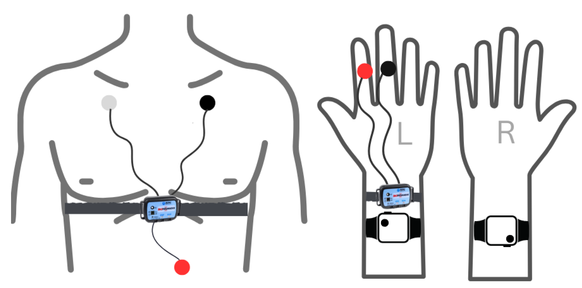
  • Electrocardiogram (ECG): Data were acquired using Biopac Bionomadix wireless device RSP&ECG (Model BN-RSPEC-TGED-T) sensors, placed on the chest in a Lead I configuration. These sensors were connected via BN-EL45-LEAD3 cables to electrodes pre-gelled with conductive gel. The red, black, and white electrodes corresponded to the positive (E+), negative (E), and ground (GND) inputs, respectively (Figure 6 chest placement).
  • Electrodermal Activity (EDA): Measurements were taken using a Bionomadix PPG&EDA (Model BN-PPGED-T) sensor. This sensor, connected via a BN-EDA25-LEAD2 cable, utilized electrodes affixed to the index and middle fingers of the left hand (Figure 6 hand placement).
To detect if the driver has their hands on the steering wheel, two inertial motion tracking MetaWear IMU sensors were positioned on both wrists to collect 3-axis accelerometer data, 3-axis gyroscope data, and Quaternion orientation values (Figure 6 hand placement).

2.3. Description of Data Acquisition and Computational Equipment

A Microsoft Surface tablet was used to acquire physiological data using AcqKnowledge (v6.0), a BIOPAC data acquisition and visualization software. To replicate realistic self-driving behavior during the experiment, CARLA was integrated with a state-of-the-art autonomous driving system [28], which controlled the vehicle’s trajectory, speed, and reaction to traffic scenarios in the virtual environment. This autonomous driving system was executed on a 15.6 Dell Precision 5570 mobile (Dell Technologies Inc., Round Rock, TX, USA) workstation equipped with an Intel Core i7-12800H vPro processor, 32 GB DDR5 4800 MHz RAM, and an NVIDIA RTX A1000 GPU with 4 GB GDDR6 dedicated memory. On the other hand, the CARLA simulator was running on an Alienware Aurora R16 desktop computer (Dell Technologies Inc., Round Rock, TX, USA) with an Intel Core i9-14900F processor (24 cores, 32 threads, base 2.0 GHz), 32 GB DDR5 RAM, 2 TB SSD storage, and an NVIDIA GeForce RTX 4070 SUPER GPU with 12 GB GDDR6 dedicated memory. Additionally, a separate touchscreen Google Pixel tablet (Google LLC, Mountain View, CA, USA) (10.95 LCD, 2560 × 1600 resolution, 267 ppi) served as the HMI device.
A multimodal dataset was collected during each experimental session to comprehensively assess driver behavior, physiological state, and attentional performance during TOR scenarios. The data acquisition system was designed to synchronize and log high-resolution information from various sources, enabling robust training and evaluation of machine learning models.
The core data streams include the following:
  • Physiological Signals (ECG and EDA): The signals were acquired in real time. Data were streamed continuously during the experiment and stored in raw .csv format for offline analysis. A custom-designed graphical interface was used for live monitoring, buffering, and data export.
    Signal processing and feature extraction were performed using NeuroKit2 (v0.2.11) (Python) and supplementary MATLAB (R2020b, Update 7) routines. The preprocessing pipeline included noise reduction, signal normalization, and event detection—specifically R-peak identification for ECG and skin conductance response (SCR) peak detection for EDA. Signals were segmented into fixed-length windows (1 min), and features were extracted to quantify physiological states associated with stress, arousal, and cognitive workload.
    The extracted features include widely used psychophysiological metrics. For example, RMSSD (Root Mean Square of Successive Differences) and SDNN (Standard Deviation of NN intervals) are time-domain indicators of heart rate variability (HRV), commonly associated with parasympathetic nervous system activity and emotional regulation. Similarly, the LF/HF ratio (Low-Frequency to High-Frequency power ratio) is a frequency-domain HRV metric frequently used as a marker of sympathetic–vagal balance. In electrodermal activity, SCL (skin conductance level) reflects tonic arousal, while SCR (skin conductance response) quantifies phasic responses to discrete stimuli or cognitive shifts. These features serve as core inputs for downstream modeling of driver attention and state classification. For a more detailed overview of the physiological metrics and their interpretation, see [29,30,31].
  • Inertial Motion Data (IMU): MetaWear sensors (MbientLab Inc., San Jose, CA, USA) on both wrists recorded accelerometer, gyroscope, and quaternion values from both wrists at  10 Hz. This data enabled hands-on-wheel detection, processed via LSTM-based deep learning models. The IMU logs were labeled with binary contact states and exported as structured CSV files. More details on this model can be found in [32].
  • Attention Logs: As illustrated in Figure 3, participants responded to visual stimuli through a gear-shift lever, with each interaction automatically recorded in .json files including both response time and accuracy. Each recorded response was subsequently scored and categorized into discrete attention levels—focused, semi-distracted, or distracted. These attention labels were then resampled and temporally synchronized with the physiological signals at 1s intervals to facilitate data fusion and training processes.
  • Simulator and Vehicle State Logs: The simulator environment recorded continuous data on vehicle trajectory, speed, TOR events, traffic objects, and user control inputs. These logs were structured via a Lightweight Communications and Marshaling (LCM) framework and timestamped for alignment.
All data files were time-synchronized using UNIX timestamps and exported in standardized CSV and JSON formats. The final dataset comprises both raw and processed versions of each modality, enabling flexible downstream analysis and integration. This rich dataset supports supervised model training, attention-state classification, and the development of a real-time driver-monitoring system. Table 2 details the characteristics extracted from each process.

2.4. Participants

The experimental protocol was conducted with N S = 30 volunteer participants, following a public call for participation distributed among the university community. Interested individuals contacted the research team and completed the informed consent process in accordance with institutional ethical protocols. The sample consisted of a balanced mix of individuals, representing a diverse range of ages, genders, and driving experiences. Specifically, 63.3% of participants identified as male and 36.7% as female. Their ages ranged from 22 to 71 years, with a mean of 36 and a standard deviation of 12.7, reflecting a diverse adult population.
Driving experience varied considerably across participants, ranging from 0.6 to 55 years, with a mean of 14.95 years and a median of 8.5 years. This variability enabled the analysis to capture the behavioral and physiological responses of both less- and more-experienced drivers. Only 13.3% of participants reported prior experience with autonomous vehicle systems, making the findings particularly relevant for those facing real-time takeover situations for the first time.
Participants were divided equally into two experimental groups (GR1 and GR2), each comprising 50% of the total sample. Both groups presented similar demographic characteristics, ensuring a balanced distribution of variables such as gender, age, driving experience, and prior experience with autonomous vehicles. Table 3 provides detailed descriptive statistics.
Each group was exposed to a different attention level configuration, as described in Table 4. This attention-state configuration was chosen for each group and experiment to simulate realistic and varied situations that could arise in conditioned autonomous driving. This configuration enables analysis of how changes in attention level, whether gradual or sudden, affect the driver’s physiological response to critical events, such as a traffic accident. This intentional variability in the data helps assess the physiological responses of different profiles to cognitive changes.

3. Data Processing and Modeling Framework

This section details the end-to-end modeling pipeline. First, the dataset is organized and standardized by curating features and applying global min–max normalization to the physiological channels (HOW remains binary). Second, this section explains how the attention target was defined for participants during the experiment. Third, subject grouping is derived with time-series k-means based on physiological parameters to form coherent clusters. Finally, an LSTM sequence-to-label architecture is specified and its hyperparameters are tuned via Bayesian optimization.

3.1. Physiological Feature Preprocessing

A multimodal dataset was created combining peripheral physiological features extracted from raw electrocardiogram and electrodermal activity with a binary driver interaction signal indicating hands on wheel. For each subject s i S , i = { 1 , , N s } , continuous ECG and EDA streams were segmented into non-overlapping windows of 1 s to derive a set of 29 physiological features in a time interval t = [ 0 , T i ] , with T i being the duration of all the driving experiments for subject i combined. In parallel, the HOW channel was sampled at 1 Hz and encoded as h t { 0 , 1 } (0: no hands on the wheel; 1: hands on the wheel). Let N F = 30 be the feature dimensionality (29 physiological features plus HOW). Each row at time t is therefore an N F -dimensional feature vector
z i t = x i t h i t , x i t R 1 × 29 , h i t { 0 , 1 } , z i t R 1 × N F .
where x i t R 29 are the physiological features and h i t the HOW indicator for the subjects s i .
To mitigate inter-subject amplitude variability while keeping feature scales comparable, a global min–max normalization was applied to the 29 physiological features and mapped them to [ 1 , 1 ] :
x ˜ j = 2 x j min ( x j ) max ( x j ) min ( x j ) 1 , j = { 1 , , 29 } ,
leaving the binary HOW feature unscaled. This [ 1 , 1 ] scaling is standard in physiological affect/stress modeling because it bounds the dynamic range and speeds up optimization [33,34].

3.2. ANOVA

To identify the physiological features most strongly associated with variations in driver attention, a one-way ANOVA was conducted between the two attention classes. This statistical test quantifies the extent to which each feature exhibits significant differences between the two conditions, providing an interpretable measure of discriminative power. Features with lower p-values indicate greater statistical relevance to the classification task, guiding subsequent comparisons and the selection of machine learning models. The ranked features according to their p-values are summarized in Table 5.

3.3. Feature Selection

In the dataset selection stage, feature dimensionality was determined through the clustering strategy described in Section 3.5 and by training the models detailed in Section 3.6.2. Based on the comparative performance across different configurations, it was concluded that using 30 features yields the most consistent and robust results, as summarized in Table 6.

3.4. Attention Level Preprocessing

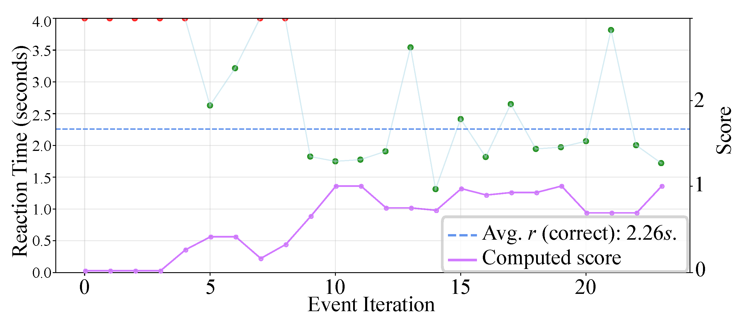
A data preprocessing pipeline was designed using the responses recorded to each attention stimulus during the experiments. It should be noted that each stimulus was presented at 20-s intervals, giving the participant a maximum of 4 s to select the correct option. The results obtained for Subject 6 are shown in Figure 7, where the red dots reflect the stimuli without response or incorrect responses, and the green dots represent correct responses. Additionally, the average correct response time for this subject was 2.26s. According to this group and the experiment (Group 1, experiment 2), the suggested attention setting for this driver corresponded to distracted–focused–focused (see Table 4).
To transform the raw responses into labels suitable for the model, a preprocessing pipeline was designed with four main steps: (1) calculate the characteristic reaction time of each subject from the correct responses, (2) determine, in each trial, if the response occurred within the individual reference time, (3) apply a penalty when the selection was incorrect, or there was a late response with respect to its individual reference, and (4) define the final attention labels at two levels: focused and distracted.
First, each reaction time r n , i (bounded to the interval [ 0 , R T max ] seconds, with R T max = 4 ) is normalized with respect to the individual average r ¯ , ensuring that the score reflects the relative performance of the driver rather than the overall speed of the group, as detailed in Equation (2):
r ¯ i = 1 N A n = 1 N A r n i score ( r n i , r ¯ ) = R T max r n i R T max r ¯ i .
where N A is the number of attention level evaluations requested during the experiment.
Once the individual yield is calculated, each attempt is labeled by a variable Y i n , where i denotes the subject and n denotes the attempt. This variable can take three values: correct where the star was selected in adequate time, incorrect where a different figure was chosen, or failed where no response was recorded within 4 s, as shown in Equation (3).
y i n = 0 = missed , score ( r i n , r ¯ ) = correct , α · score ( r i n , r ¯ ) = incorrect ,
where α = 0.5 is a weighting coefficient introduced to penalize incorrect responses. This choice ensures that errors, even if produced with fast reaction times, contribute less to the overall score than correct answers, but are not entirely disregarded; this computed score can be seen reflected in Figure 7, where each response is compared with its score for each stimulus.
From y i n , two attention levels are defined in Equation (4):
a i n = y i n < τ = distracted , y i n τ = focused ,
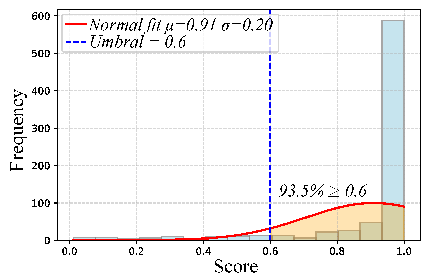
where the threshold τ = 0.6 was established by analyzing the distribution of scores obtained only from correct answers, which is illustrated in Figure 8. This distribution is visualized by the light blue histogram bars, which indicate the frequency of each score. Fitting a Gaussian function (orange line with μ = 0.91 σ = 0.20 ) to showed that 93.5 % of the values were above the threshold, which is represented by the dashed blue vertical line at τ = 0.6 and highlighted by the orange shaded area. This value enabled distinguishing between correct answers associated with high concentration (higher scores) and those slower than the average response time, which could indicate a lower level of sustained attention. It also balanced the proportions of instances labeled as focused and distracted to avoid bias towards a single class.
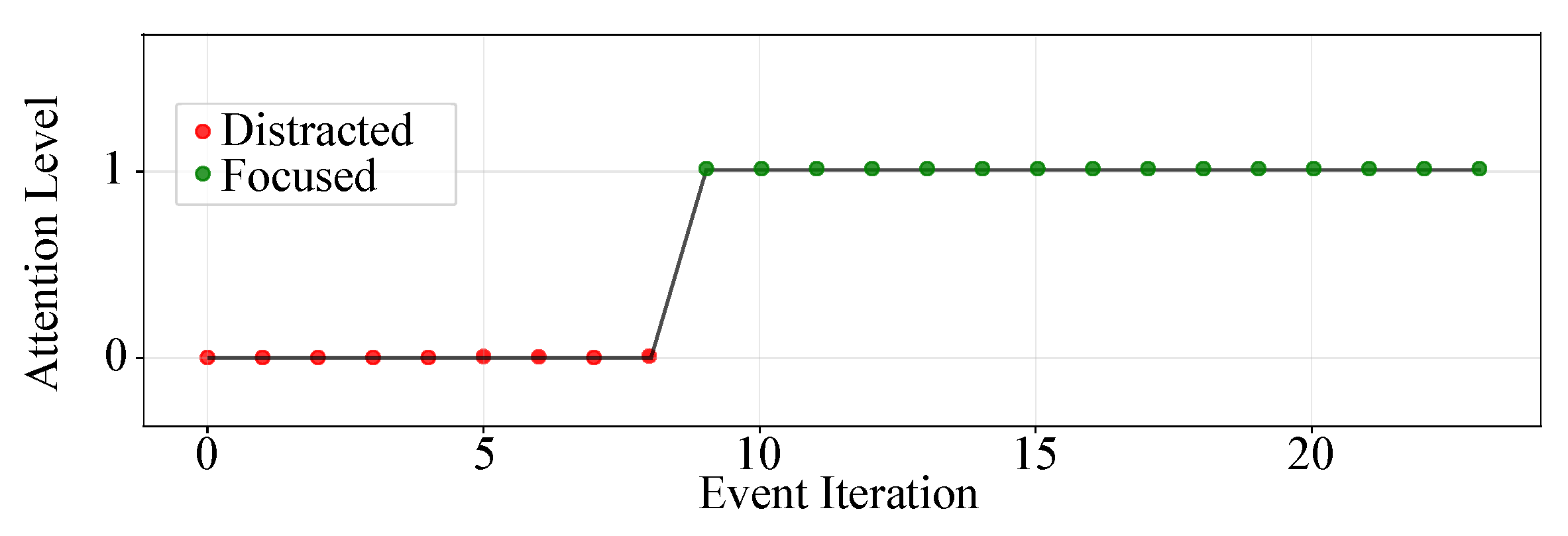
In this way, each attempt is categorized at one of two levels of attention: focused when the answer was correct and in adequate time, or distracted when the answer was late, incorrect, or nonexistent. This scheme ensures that the data are consistent, equivalent, and aligned with the cognitive relevance of each moment, as illustrated in Figure 9.

Hands-on-Wheel Prediction Feature Preprocessing

The hands-on-wheel (HOW) signal was incorporated as an auxiliary feature derived from a previously developed LSTM-based detector [32].
Let b = 0 , 1 , 2 , index samples with t b = b · 0.1 s . Define the HOW label h b { 0 , 1 }  as
h b = 1 , if hands are on the wheel at t b , 0 , otherwise .
Due to the LSTM’s 10 Hz output rate, the HOW stream was downsampled to 1 Hz to match the 1 s resolution of the physiological dataset: each 1 s window averages its ten samples and thresholds the mean at 0.5 to yield a binary label (1 = hands on wheel, 0 = otherwise).
The resulting data was aligned by timestamp, and the HOW series was appended as an additional column to the feature matrix used for model training.

3.5. Time-Series k-Means Clustering

To analyze each driver’s behavior, a time-series clustering strategy was employed, as it leverages the sequential structure of the data and yields more representative groupings than strategies based on single values, such as classic k-means [35]. In particular, the time-series k-means algorithm was used, which transforms the sequences into a set of clusters defined by centroids that represent similar temporal patterns [20].
Before applying the clustering algorithm, each series was normalized to the range [−1, 1]. Then, the data from experiments 1 and 2 for each subject were combined to form a time series, as shown in Equation (5).
x ^ t i x = 2 · x t i x min i S x t i x max i S x t i x min i S x t i x 1
where x t i x is the value of the feature (x) for subject (i) at time (t), and x ^ t i x represents the normalized value. The operators min ( x t i x ) and max ( x t i x ) represent the global minimum and maximum found for the feature, respectively. These were calculated considering all subjects i S and all times t. Comparability between characteristics with different magnitude ranges is ensured this way.
In this study, drivers completed the experiments at different time intervals, generating sequences of varying lengths. For this reason, instead of using a Euclidean distance metric, dynamic time warping (DTW) was chosen, a measure that allows aligning time series of different durations or with possible distortions on the time axis, although its computational cost is higher.
The k-means clustering algorithm seeks to assign data to clusters and position centroids such that the sum of all squared distances is as small as possible [36], as shown in its objective equation:
J i = min { u i k } i = 1 N S x = 1 N F 1 k = 1 N K u i k x ^ t i x c t k x 2 ,
where x ^ t i x is the normalized value of the physiological parameter x for subject i at time t, c t k x is the corresponding value of the centroid of cluster ς K , with K denoting the set of N k clusters. Finally, u i k is the membership indicator, which takes the value 1 if subject i belongs to cluster ς k , k [ 1 , , N k ] and 0 otherwise. In this context, the objective function measures the total cost of clustering. It is obtained by minimizing the sum of the squared distances between the subjects’ series and the centroids of their respective clusters.
One of the most commonly used strategies for determining the optimal number of clusters is the elbow plot, which identifies the point at which the inertia (the sum of squared intra-cluster distances) stops decreasing significantly. On the other hand, the silhouette score, which measures how compact and separated the clusters are, reaches higher values when the data are well grouped and differentiated. In this work, both metrics are employed in a complementary manner: the elbow plot is used to determine the number of clusters, and the maximum value of the silhouette index confirms the final choice.
To validate this choice of N k , a strategy was implemented that simultaneously evaluates stability and silhouette in time-series clustering. The analysis is based on the clustering stability principle, which states that a partition is stable if it produces consistent results in the face of slight data perturbations [37]. This principle, widely demonstrated for the K-means algorithm, can be extended to TimeSeriesKMeans, given that both share a centroid-based nature [37]. Unlike supervised classification methods, where there is a “ground truth” that guides the evaluation, in unsupervised clustering, stability is considered a meta-principle that allows estimating the reliability and reproducibility of the structure found.
To generate perturbed versions of the original dataset N S , the bootstrap method is used, taking 80 %   ( λ = 0.80 ) of the data in B = 50 replicates. In each replicate b, a cluster C b is obtained.
The observed stability is calculated as the average distance between all pairs of obtained clusters, using the Adjusted Rand Index (ARI) based on the intersection of the data points that coincide in the two subsamples. The observed average instability is theoretically defined in Equation (7) [37].
Instab ( k , n ) = 1 b max 2 b , b = 1 b max d ( C b , C b ) ,
where a higher ARI value indicates greater stability and reproducibility between the obtained clusters. It is essential to normalize stability, as instability tends to increase systematically with the number of clusters (k). To correct this bias, a null baseline was used, obtained by repeating the stability calculation, comparing partitions with randomly shuffled labels but preserving the original cluster size.
From this adjustment, the final selection of K is based on two key metrics that assess the significance of the observed stability compared to this null model: the Stability Gap and the Z-score Stability. Thus, the Stability Gap is defined as the difference between the observed stability and the expected stability under the null model, as seen in Equation (8), while the Z-score Stability evaluates whether the actual stability is significantly greater than the null Equation (9). Finally, the value of K that produces the highest Z-score Stability is considered to be the most statistically significant number of clusters [37].
Stability Gap = mean obs mean null ,
Z - score Stability = ( mean obs mean null ) std null .
In this way, to define whether a new subject belongs to one of the defined clusters, the same processing flow applied during training is followed. First, physiological and behavioral signals are recorded during the experiments. Subsequently, the series are preprocessed and normalized to the range [−1, 1] to ensure compatibility with the original model’s scale. Finally, the normalized sequences are evaluated using the pre-trained TimeSeriesKMeans model, assigning each subject to the cluster whose centroid has the lowest dynamic time warping (DTW) distance. This procedure allows new individuals to be classified without retraining the model, preserving consistency with the original segmentation.
In addition to the time-series k-means-based strategy, an alternative approach combining principal component analysis and K-means was implemented. In this case, the physiological datasets were transformed using principal components analysis. This multivariate technique seeks to reduce the dimensionality of the data by identifying a set of uncorrelated components that account for most of the original variance [38]. This transformation allows the data to be represented in a lower-dimensional space, facilitating comparisons between subjects and the detection of overall similarity patterns. K-means was applied to this data reduction to perform clustering, using the principal components rather than the entire sequences. However, this strategy provides a general view of the data structure.

3.6. Model Architecture and Hyperparameter Optimization

This section describes the Long Short-Term Memory (LSTM) model architecture and the Bayesian optimization implemented in this study.

3.6.1. Random Forest and Support Vector Machine

Two classical machine learning models were evaluated for attention level classification: Random Forest (RF) and Support Vector Machine (SVM). The best configuration for the RF model was Splits = 25, Cycles = 150, and Learning rate = 0.01, which provided a stable balance between model complexity and performance. For the SVM model, the optimal configuration used a Radial Basis Function (RBF) kernel with BoxConstraint = 0.10 and KernelScale = 0.10, achieving consistent results across subjects.

3.6.2. Long Short-Term Memory Architecture

The attention level was modeled from physiological time series using an LSTM network, a recurrent architecture designed to capture short- and mid-term temporal dependencies in sequential data [39]. The suitability of LSTM-based pipelines for driver vigilance and drowsiness using peripheral physiology (e.g., ECG/respiration) has been demonstrated in recent work, supporting the choice of a temporal model for this task [40].
Figure 10 summarizes the end-to-end model. First, the physiological features are min–max normalized to [ 1 , 1 ] as detailed in Section 3.1. The normalized sequences are then processed by an LSTM-based sequence-to-label classifier with a last-step readout and a compact feedforward head, as depicted in the figure.
Windows were built at 1 Hz according to Welch PSD analysis, which showed that over 96% of the physiological features’ spectral power lies below 0.1 Hz, confirming that 1 Hz sampling effectively captures the relevant dynamics without oversampling. Accordingly, sequences of length L = 5 s with a stride of r = 1 s were used to capture short-term temporal dependencies while preserving sufficient temporal resolution.
For each subject ( s i ) with ( t = 1 , , T i ) one-second samples and feature vectors z i t R N F , the set of valid window start indices is
Q i = { 1 , 1 + r , 1 + 2 r , , T i L + 1 } .
Given any q Q i , the length-L window is defined as the concatenation of L consecutive time steps,
W i q = z i q , z i ( q + 1 ) , , z i ( q + L 1 ) R N F × L .
Windows are constructed for the combined experiments of each subject ( s i ) (two experiments per subject), so no window crosses subject or experiment boundaries.
The resulting sequences are processed by a unidirectional, causal LSTM with a last-step readout (Figure 10). A compact feedforward head then maps the sequence summary to two logits, which are converted to posterior class probabilities via a softmax. Batch normalization is applied at the network input to stabilize feature scales across subjects and sessions, and dropout is used around the recurrent and dense blocks to mitigate overfitting without inflating model size. Optimization was performed using categorical cross-entropy and the Adam algorithm over 30 epochs, with mini-batches of 64 and shuffling at every epoch.
To assess subject-independent performance, i.e., generalization across individuals, Leave-One-Subject-Out (LOSO) cross-validation was employed. This protocol is widely recommended in physiology-based affect and stress recognition because it mitigates optimistic bias associated with subject overlap and better reflects deployment to unseen users. Recent studies explicitly advocate for LOSO for fair evaluation in wearable physiology and emotion/stress modeling [34,41,42]. In particular, [43] demonstrated the necessity of LOSO for EEG-based disease diagnosis using a dataset of approximately 30 participants, showing that conventional k-fold cross-validation can substantially overestimate performance due to data leakage across subjects. Similarly, [44] employed a multi-input CNN-LSTM architecture for fear-level classification from EEG and peripheral physiological signals using a dataset of comparable size, emphasizing the importance of LOSO evaluation to ensure realistic cross-subject generalization. Following these recommendations, LOSO validation was applied in the present study to maximize the use of the available data while strictly preventing overlap between training and testing subjects. Accordingly, the reported results were aggregated to the arithmetic mean across all LOSO folds, with one fold per held-out subject.
After evaluating the three supervised models (Random Forest, SVM, and LSTM) with accuracies of 84.93%, 62.25%, and 95.12%, respectively, the LSTM model was selected for further analysis. Its superior performance indicates a better alignment with the temporal characteristics of the physiological data, making it the most appropriate approach for this study.

3.6.3. Bayesian Optimization

Deep learning models for time series, including LSTM architectures, are sensitive to hyperparameter choices (e.g., sequence length, hidden width, learning rate, dropout rate, and optimizer). Manual trial-and-error tuning across a large, multidimensional space is laborious and error-prone, and it often fails to identify strong configurations under realistic compute budgets. Evidence from time-series forecasting, as well as from driving and driver-state monitoring, indicates that automated hyperparameter search enhances performance and efficiency compared to manual heuristics, thereby mitigating degradation due to suboptimal settings [17,45,46].
In advanced driving assistance and autonomous driving contexts, training deep temporal models is computationally expensive. Prior studies report that Bayesian optimization can improve spatiotemporal LSTM models for steering prediction and driver monitoring by locating better hyperparameters with fewer trials than manual search [17,46]. These characteristics motivate a sample-efficient optimizer capable of handling noisy, non-convex objectives under limited evaluation budgets.
Building on this rationale, the end-to-end pipeline (windowing, normalization, and subject-aware validation) is formalized as a black-box objective. Bayesian optimization with an expected improvement family acquisition guides the selection of each costly training run, and the resulting hyperparameters are reported both at the global level and per cluster. This procedure replaces ad hoc heuristics with a reproducible search designed to target cross-subject generalization in physiological driver-state modeling [17,45,46,47,48].
Bayesian optimization was used to automatically select the hyperparameters of the LSTM classifier shown in Figure 10. The set of hyperparameters is
θ = { window size , LSTM layer units , fully connected units , dropout , learning rate } .
Window size defines the temporal length of each input sequence, LSTM layer units determine the number of hidden units in the recurrent layer, fully connected units specify the width of the projection layer, dropout controls the fraction of activations dropped during training, and learning rate sets the step size of the Adam optimizer.
The training and validation pipeline is treated as a black-box function O ( θ ) . For each candidate θ , the model is trained with reduced epochs and validated using subject-wise K-fold cross-validation. Let Acc m ( θ ) be the accuracy on fold m = [ 1 , , M ] . The objective is defined as the negative of the average accuracy across folds:
O ( θ ) = 1 M m = 1 M Acc m ( θ ) .
A Gaussian process surrogate is fitted to past evaluations { ( θ j , O ( θ j ) ) } . Based on this surrogate, the expected improvement plus acquisition function selects the next hyperparameter configuration by balancing exploration and exploitation. This iterative process continues until the evaluation budget is exhausted. The best observed configuration θ is then retrained with an enlarged epoch budget, and its accuracy is reported as the final result. Once the optimal configuration is found, the model is retrained with a larger epoch budget for reporting purposes. Random seed initialization was fixed when assigning subjects to folds to enhance reproducibility.
This protocol aligns with standard practice in physiological modeling and driver-state monitoring, where inter-subject variability is substantial [48,49].

4. Results

First, several machine learning models, RF, SVM, and LSTM, were compared to determine the most suitable architecture for the classification task. Once the optimal model was selected, the set of subjects was clustered based on their physiological profiles using the strategy described in Section 3.5 to obtain the optimal number of clusters and analyze the features of each of them. Then, the LSTM model is applied to each cluster. The performance of these cluster-specific models is evaluated by comparing them with that of a global model that includes all drivers in the dataset. First, the global model was trained using the original hyperparameters; second, Bayesian optimization was applied to the global model to obtain the global reference. Finally, the physiology-based clusters are also compared against non-physiological partitions; four additional cluster pairs were defined: sex (female, male), driving experience (experienced, novice), and two random pairs.

4.1. Clustering

Once the dataset with the normalized series was prepared, the optimal number of clusters was determined. To accomplish this, the inertia obtained by varying the number of clusters from N k = 1 to N k = 9 was evaluated, as illustrated in Figure 11a. This upper bound was chosen because the dataset comprised 30 participants, and allowing more than 9 clusters would result in very small groups with limited representativeness. The objective of this analysis was to identify the point at which the inertia stops decreasing significantly, thus avoiding excessive oversegmentation of the data and ensuring an appropriate balance between simplicity and representativeness of the clustering model.
Figure 11a shows that, for N k = 2 and N k = 3 , the inertia reaches relatively low values, while from N k > 3 , the reduction is no longer significant. For its part, the silhouette score (Figure 11b) shows a pronounced drop between N k = 2 and N k = 3 , remaining at considerably lower values for N k > 3 . However, the most determining criterion comes from the stability analysis in Table 7, which shows that N k = 2 presents the greatest consistency between executions (Figure 11c), indicating that the clustering structure is robust against perturbations of the dataset. Considering stability, silhouette, and inertia together, it is concluded that the optimal number of clusters for this dataset is N k = 2 , where the best balance between separation, compactness, and clustering reproducibility is achieved. Similarly, for the stability tests used for the dataset with noise in the physiological signals, an average stability was obtained for k = 2 of 0.88 , for k = 3 of 0.504 , and for k = 4 of 0.529 .
Once the optimal number of clusters was determined, the time-series k-means algorithm with DTW distance was applied, configured to divide the set into two groups ( N k = 2 ). The model described in Section 3.5 was trained for a maximum of 50 iterations, with a random state of 42 points to ensure stable, reproducible results. This procedure allowed each time series to be assigned a cluster label and, at the same time, to calculate the representative centroids of each group, from which Table 8 was obtained.
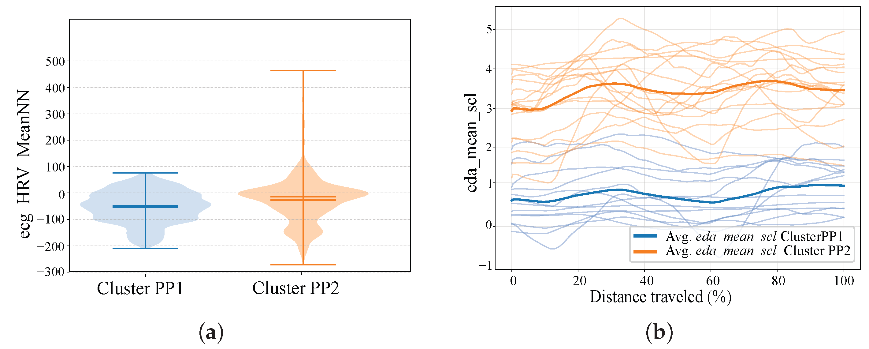
The clustering results identified two physiological parameter (PP) clusters (Cluster PP1 and Cluster PP2), allowing recognition of specific patterns associated with each group. An example of the physiological differences among clusters is depicted in Figure 12a. It shows how Cluster PP1 included subjects who, for the most part, presented negative mean heart rate variability values and low electrodermal conductance levels. This may indicate lower autonomic activation during the driving task for most of the subjects. In contrast, in Figure 12b, Cluster PP2 (orange line group) included participants with greater heterogeneity in their ECG values, some with elevated positive averages, and consistently higher EDA levels, reflecting a profile of greater physiological activation. Regarding demographic characteristics, both clusters included a mix of young men and women, indicating that age and driving experience were not directly associated with cluster membership. This suggests that the observed physiological dynamics primarily explain the cluster separation.

4.2. Results of Bayesian Optimization

The Bayesian optimization described in Section 3.6.3 was applied consistently at both the global and cluster levels. For all cases, the hyperparameters shown in Figure 10 served as the base configuration, and the procedure refined these settings to accommodate between-subject and subpopulation variability.
The hyperparameters are tuned as depicted in Table 9: (i) Window size (sequence length/temporal receptive field), (ii) LSTM units (recurrent hidden width), (iii) Dropout, (iv) Fully Connected Layers (projection width), and (v) Learning rate (searched on a logarithmic scale due to multiplicative effects). This design keeps the search expressive yet tractable for expensive sequence models.

4.3. LSTM Results

This subsection reports the LSTM results for the global model and for the cluster-specific models under a standard LOSO evaluation protocol. For each cluster, a separate Bayesian optimization was conducted within the same search space (LSTM layer units, fully connected units, dropout, learning rate) and with the same training protocol (Table 9).
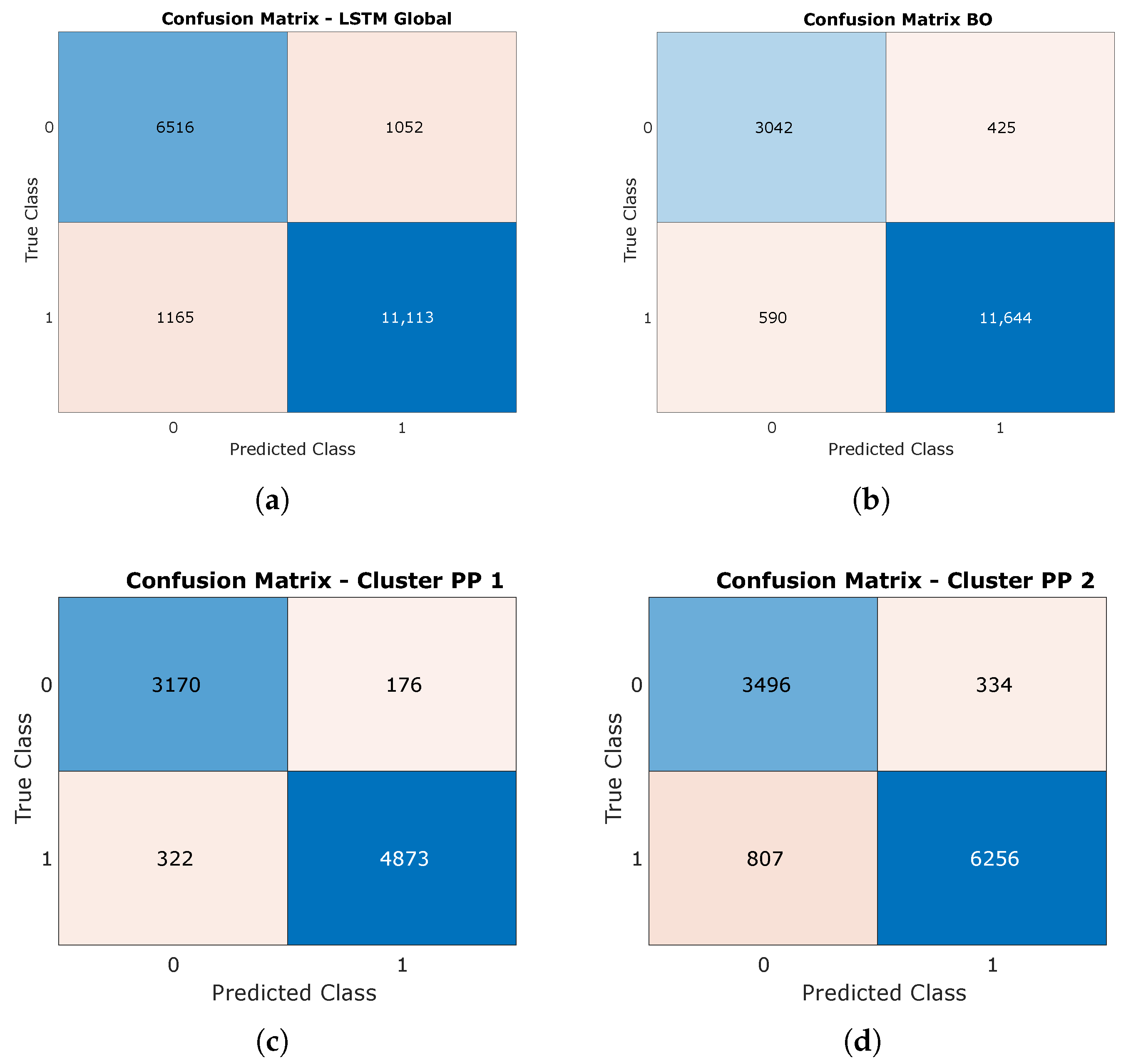
Results are presented at two levels. First, the confusion matrices and derived metrics for the global model are given, as well as clusters PP1 and PP2. Secondly, the percentage differences relative to the global baseline are described to quantify subject-wise changes attributable to cluster specialization.
Figure 13a shows the confusion matrix of the global LSTM before Bayesian optimization, yielding an overall accuracy of 88.83 % . From these counts, the per-class F 1 scores are 90.93 % for Attention (class 1) and 85.46 % for No-attention (class 0), with a macro F 1 of 88.20 % . Qualitatively, the model is stronger on class 1, with some class 0 samples misclassified as class 1.
Figure 13b shows the confusion matrix of the LSTM after Bayesian optimization. The pooled accuracy is 94.00%. From these counts, the per-class F 1 scores are 95.8% for Attention (class 1) and 85.7% for No-attention (class 0), yielding a macro F 1 of 90.8%. Compared with the pre-optimization model (accuracy 88.83 % , macro F 1 = 88.20 % ), both overall accuracy and macro F 1 show clear improvements, while the total misclassifications ( F P + F N ) slightly decrease from 1076 to 1015, confirming that the Bayesian-optimized configuration enhances class discrimination and overall generalization.
Figure 13c reports PP1 under pooled LOSO aggregation. The model achieves a global accuracy of 94.17%. Class-wise F 1 scores are 92.72% for class 0 (No-attention) and 95.14% for class 1 (Attention), yielding a macro F 1 of 93.93%. The small gap between classes suggests a well-balanced behavior.
Figure 13d summarizes PP2 in the same pooled setting. The model attains 89.53% global accuracy and records F 1 scores of 85.97% for class 0 and 91.64% for class 1, for a macro F 1 of 88.81%. Performance remains solid, with a clearer advantage on the Attention class relative to No-attention.
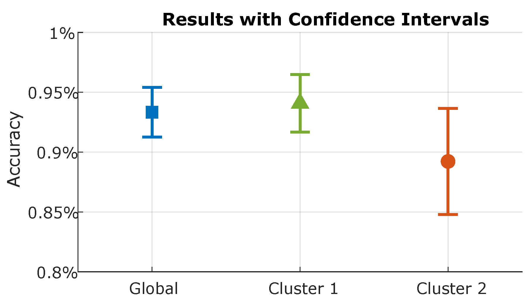
Figure 14 presents the mean subject-wise accuracy with 95% confidence intervals obtained under the LOSO validation scheme for the global model and the two cluster-specific models, together with the subject-matched comparison of each cluster relative to the global configuration. The global model (blue) reached an overall accuracy of 93.33% with a narrow confidence interval of ±2.08 percentage points, showing stable performance across all subjects. Cluster 1 (green) achieved 94.08% with a confidence interval of ±2.40 percentage points, while Cluster 2 (orange) reached 89.22% with a wider interval of ±4.44 percentage points. Although the global model exhibits the most stable average behavior, the cluster-based configurations capture subject-specific dynamics that can enhance performance within more homogeneous participant groups.
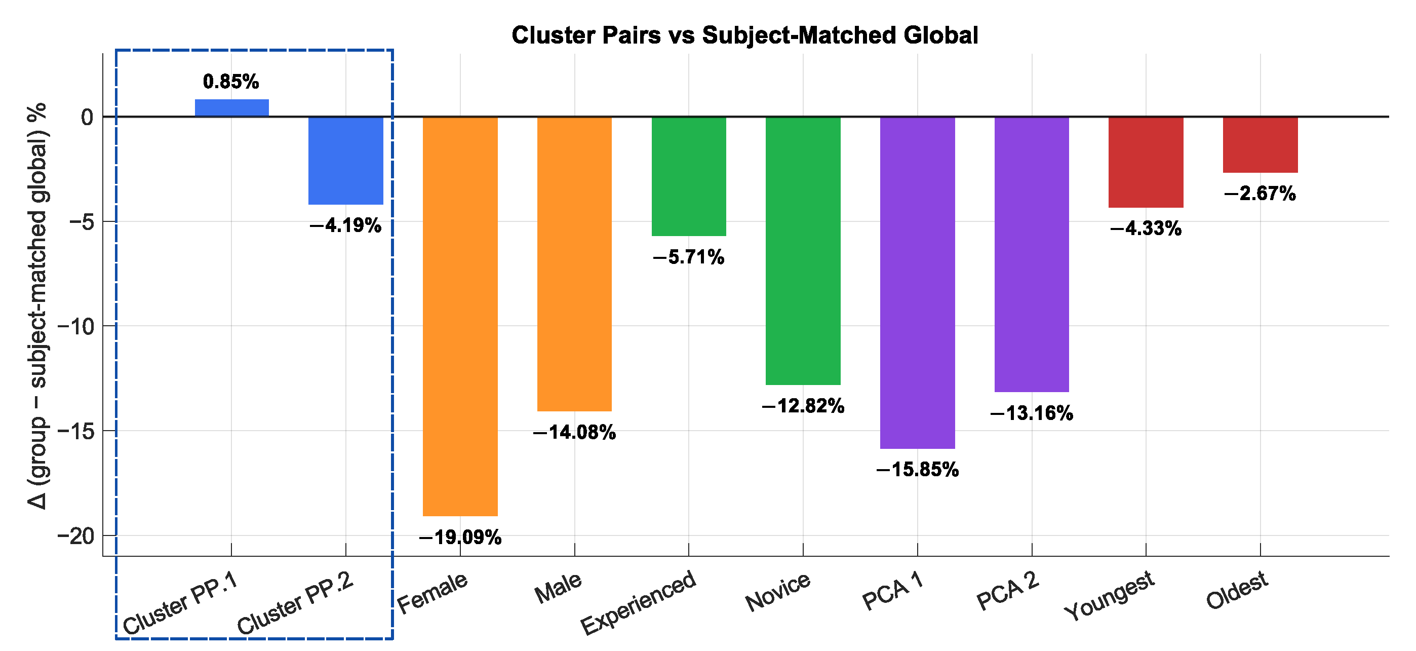
Figure 15 presents an analysis that compares each cluster against a subject-matched global reference. Each bar shows the difference in average LOSO accuracy for the subjects in that cluster when evaluated with their cluster model versus the same subjects evaluated with the global model. Positive values indicate that the cluster outperforms the subject-matched global reference; negative values indicate the opposite.
Colors denote partition families: blue corresponds to physiology-driven clusters, yellow to gender-based clusters, green to driving-experience clusters, purple to PCA-based clusters, and red to age partitions. Within each color, the two bars represent the two clusters that form the pair. The dashed blue rectangle highlights the physiology-driven pair, which achieves the best performance among the other partition families shown. The blue dashed square highlights the pair of clusters identified using the TimeSeriesKMeans method.
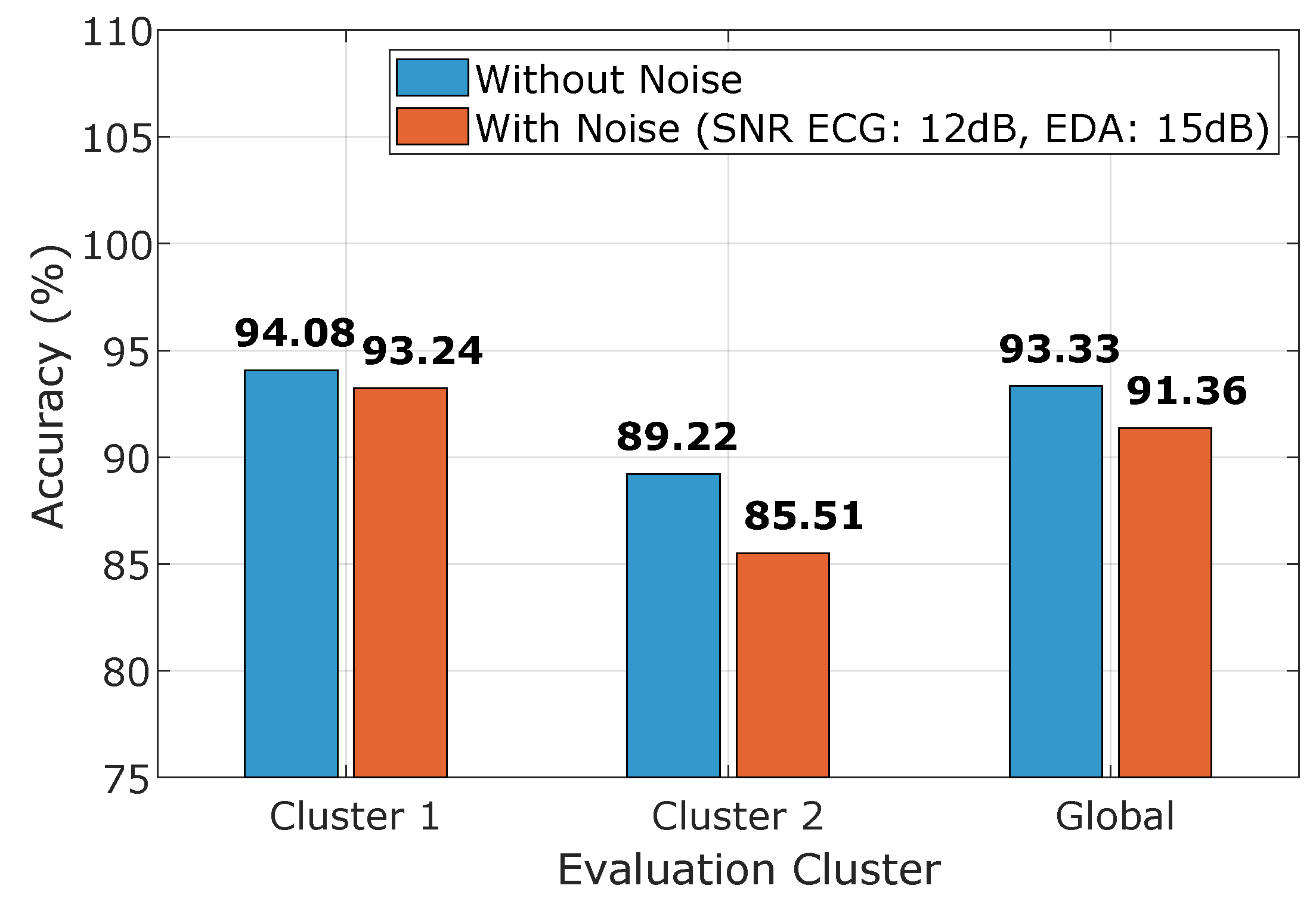
To evaluate the robustness of the LSTM model to signal noise, Additive White Gaussian Noise (AWGN) was systematically introduced to the ECG and EDA signals in the dataset. Based on the literature, a fixed Signal-to-Noise Ratio (SNR) of 12 dB was applied to the ECG signals. For the EDA signals, a fixed SNR of 15 dB was used, which falls within the range of low- to high-SNR conditions explored in previous studies [50,51,52]. After augmenting the dataset with this controlled noise, the performance of the LSTM model was evaluated using the same architecture as with the original, clean signals. The evaluation yielded nearly identical results as is shown in Figure 16, with accuracies of 93.24% for Cluster 1, 85.51% for Cluster 2, and a global accuracy of 91.36%.
Table 10 shows that the cluster-specific models present a lower computational load per physiological window compared with the global configuration. Cluster 1 and Cluster 2 reduce the total number of operations by approximately 25–27%, mainly in the recurrent (LSTM) component, which accounts for more than 98% of the total FLOPs in all models. Despite this reduction, both clusters maintain sub-millisecond inference times ( 0.10 ms per sample) and comparable throughput ( 9.6 9.7 k samples/s) to the global model while preserving an almost identical memory footprint ( 0.3 MB ). These results indicate that the cluster architectures provide a more compact and computationally efficient representation of physiological dynamics within groups of subjects sharing similar ECG and EDA characteristics.

5. Discussion

The decision to retain two clusters for the analysis was based on a balance between validating internal metrics and ensuring the stability of the clustering model. Joint analysis of the elbow graph (Figure 11a) and the silhouette index (Figure 11b) showed that N K = 2 simultaneously achieved a significant reduction in inertia and the maximum silhouette value, demonstrating a well-defined structure and a clear separation between physiological groups. This consistency is complemented by statistical criteria that ensure the stability and generalization capacity of the predictive model. In this configuration, the clusters maintain sufficient size and adequate internal variability.
Furthermore, the stability observed for k = 2 was maintained even when the physiological ensembles were generated with different levels of random noise. This result indicates that the separation between groups is not due to minor signal fluctuations or instrumental perturbations, but rather, it reflects a consistent physiological organization. In theoretical terms, this resistance to noise suggests that the centroids of both groups are sufficiently distant in feature space to maintain their statistical identity, even in the face of local variations in signal amplitude or temporal dynamics. Additionally, this stability analysis was repeated on the same dataset after introducing a controlled level of noise into the physiological signals.
It is important to analyze whether the dataset size also influenced the definition of the number of clusters. With a sample of this size, increasing k results in groups that are too small, with few subjects per category, reducing internal diversity and the likelihood of identifying consistent physiological patterns. Conversely, maintaining two clusters allows for a balance between group separation and the representativeness of the signals within each cluster. In the future, as the dataset expands and a more diverse sample becomes available, it will be necessary to re-evaluate the clustering structure. A larger number of participants could reveal additional physiological subgroups, allowing for a more detailed characterization of attentional responses and increasing the predictive capacity of the models. However, in the current context, empirical and statistical evidence clearly supports that K = 2 represents the most coherent, robust, and generalizable solution.
It is essential to highlight that the groups obtained do not match the demographic variables considered in the experiments, such as age, sex, or driving experience. This reinforces the idea that the separation is primarily due to physiological patterns. In this sense, the two clusters show apparent differences in stimulus reception; Cluster PP1 shows negative values for feature ecg_HRV_MeanNN and low levels of eda_mean_scl, suggesting a more stable profile but lower electrodermal activation. On the other hand, Cluster PP2 exhibits greater dispersion in ecg_HRV_MeanNN, with subjects reaching very high or very low values, accompanied by consistently higher eda_mean_scl levels. This pattern could indicate that participants in Cluster PP2 were more receptive to the experimental stimuli or experienced greater physiological activation, an aspect worth exploring in future studies. On the other hand, applying dimensionality reduction using PCA before clustering resulted in more clusters, but with lower physiological coherence. This is explained because PCA summarizes the signal information into values that represent its overall variance, without fully preserving the temporal structure or dynamic transitions.
The global LSTM optimized model establishes a firm reference, and the clustering experiments indicate that specialization yields selective benefits. One cluster consistently attains the highest subject-wise performance among the partitions considered. In contrast, its companion cluster averages below the global baseline, mainly because a small subset of participants within that group performs poorly. Demographic splits and random pairs do not match the best cluster.
The Bayesian optimization stages further indicate that each cluster benefits from different regions of the hyperparameter space, suggesting that model capacity, regularization, and sequence length interact with the temporal statistics of the cluster. This interaction helps explain why a single global setting cannot be optimal for all subjects and why cluster-specific tuning attains selective gains without relying on cluster size. The Bayesian optimization budget can be deepened by expanding the hyperparameter search space and increasing the iteration count, enabling a more thorough exploration of sequence length, hidden width, depth, dropout, learning rate, and fusion choices while keeping the evaluation procedure unchanged.
A limitation of this study is the number of participants, which may constrain the full representation of physiological diversity in the dataset. While the current results demonstrate consistent performance and meaningful clustering behavior, a larger sample size could further enhance cluster robustness and model generalization. Increasing the participant pool in future studies would allow a broader range of physiological variability, leading to more stable and representative clusters. In parallel, exploring architectures tailored to each cluster and conducting more extensive hyperparameter searches across sequence length, network depth and width, regularization, and fusion strategies may further enhance cluster performance without altering the evaluation protocol.

6. Conclusions

With respect to H1 (cluster models can optimize and improve the global baseline), the evidence supports the use of cluster specialization to raise subject-wise performance when the partition captures consistent physiological structure. Gains are not universal across all clusters, indicating that improvement is conditional on the quality of the grouping rather than guaranteed by mere partitioning.
Regarding H2 (physiology-based grouping can be superior to demographic or random partitions), the results favor clusters derived from physiological features over demographic or random splits. The advantage appears to arise from the structure in the ECG/EDA dynamics and the hands-on-wheel signal, rather than from group size or coverage, which explains why non-physiological partitions tend to reproduce the global behavior.
As a practical takeaway, clustering is a viable approach to improving attention estimation when subjects share compatible physiological dynamics, while the global model remains a safe fallback in other cases.

Author Contributions

Conceptualization, J.F.M.-L., J.C.P., and E.V.; methodology, J.F.M.-L., J.C.P., E.V., and G.A.F.-C.; software, J.C.P., E.V., and A.N.; validation, J.C.P., E.V., G.A.F.-C., A.N., and J.F.M.-L.; formal analysis, J.F.M.-L., J.C.P., E.V., and A.N.; investigation, J.F.M.-L., J.C.P., E.V., A.N., and G.A.F.-C.; resources, J.F.M.-L., J.C.P., E.V., and G.A.F.-C.; data curation, J.C.P., E.V., and A.N.; writing—original draft preparation, J.C.P., E.V., G.A.F.-C., and J.F.M.-L.; writing—review and editing, J.F.M.-L., J.C.P., E.V., A.N., and G.A.F.-C.; visualization, J.C.P., E.V., G.A.F.-C., A.N., and J.F.M.-L.; supervision, J.F.M.-L.; project administration, J.F.M.-L.; funding acquisition, J.F.M.-L. All authors have read and agreed to the published version of the manuscript.

Funding

This research received financial support from the NSF EPSCoR Center for the Advancement of Wearable Technologies (CAWT) under Grant No. OIA-1849243. It was also supported in part by the CAHSI–Google Institutional Research Program.

Institutional Review Board Statement

The study was conducted in accordance with the Declaration of Helsinki and approved by the Institutional Review Board of the University of Puerto Rico (protocol code 2024100041, 25 October 2024).

Informed Consent Statement

Informed consent was obtained from all subjects involved in the study.

Data Availability Statement

The data presented in this study are available on request from the corresponding author due to the privacy terms agreed with the Institutional Review Board.

Acknowledgments

During the preparation of this study, the authors used Python Neurokit2 for data processing, Matlab 2020 for training learning models, Python 3 for clustering and data visualization, and CARLA 0.9.15 for driving simulation. The authors have reviewed and edited the output and take full responsibility for the content of this publication.

Conflicts of Interest

The authors declare no conflicts of interest. The funders had no role in the design of the study; in the collection, analyses, or interpretation of data; in the writing of the manuscript; or in the decision to publish the results.

Abbreviations

The following abbreviations are used in this manuscript:
BILSTMBidirectional LSTM
BOBayesian optimization
CARLACar Learning to Act
DTWDynamic time warping
ECGElectrocardiogram
EDAElectrodermal activity
FRFrequency
HFHigh frequency
HMIHuman–machine interface
HOWHands on wheel
HRVHeart rate variability
IMUInertial motion data
LCMLightweight Communications and Marshaling
LFLow frequency
LSTMLong Short-Term Memory
LOSOLeave-One-Subject-Out
PCAPrincipal component analysis
PPPhysiological parameter
RMSSDRoot Mean Square of Successive Differences
SCLSkin conductance level
SCRSkin conductance response
SDNNStandard deviation of NN intervals
TORTakeover requests

References

  1. Aminosharieh Najafi, T.; Affanni, A.; Rinaldo, R.; Zontone, P. Driver attention assessment using physiological measures from EEG, ECG, and EDA signals. Sensors 2023, 23, 2039. [Google Scholar] [CrossRef] [PubMed]
  2. Veluchamy, S.; Michael Mahesh, K.; Muthukrishnan, R.; Karthi, S. HY-LSTM: A new time series deep learning architecture for estimation of pedestrian time to cross in advanced driver assistance system. J. Vis. Commun. Image Represent. 2023, 97, 103982. [Google Scholar] [CrossRef]
  3. Kashevnik, A.; Lashkov, I.; Ponomarev, A.; Teslya, N.; Gurtov, A. Cloud-based driver monitoring system using a smartphone. IEEE Sens. J. 2020, 20, 6701–6715. [Google Scholar] [CrossRef]
  4. Schwarz, C.; Gaspar, J.; Miller, T.; Yousefian, R. The detection of drowsiness using a driver monitoring system. Traffic Inj. Prev. 2019, 20, S157–S161. [Google Scholar] [CrossRef]
  5. Daza, I.G.; Bergasa, L.M.; Bronte, S.; Yebes, J.J.; Almazán, J.; Arroyo, R. Fusion of optimized indicators from Advanced Driver Assistance Systems (ADAS) for driver drowsiness detection. Sensors 2014, 14, 1106–1131. [Google Scholar] [CrossRef]
  6. SAE International. Taxonomy and Definitions for Terms Related to Driving Automation Systems for On-Road Motor Vehicles (Surface Vehicle Recommended Practice: Superseding J3016 sep 2016); Technical report; SAE International: Warrendale PA, USA, 2016. [Google Scholar]
  7. Gold, C.; Körber, M.; Lechner, D.; Bengler, K. Taking Over Control From Highly Automated Vehicles in Complex Traffic Situations: The Role of Traffic Density. Hum. Factors 2016, 58, 642–652. [Google Scholar] [CrossRef]
  8. Kumar, M.; Weippert, M.; Vilbrandt, R.; Kreuzfeld, S.; Stoll, R. Fuzzy evaluation of heart rate signals for mental stress assessment. IEEE Trans. Fuzzy Syst. 2007, 15, 791–808. [Google Scholar] [CrossRef]
  9. Noh, Y.; Kim, S.; Jang, Y.J.; Yoon, Y. Modeling individual differences in driver workload inference using physiological data. Int. J. Automot. Technol. 2021, 22, 201–212. [Google Scholar] [CrossRef]
  10. Nezamabadi, K.; Sardaripour, N.; Haghi, B.; Forouzanfar, M. Unsupervised ECG Analysis: A Review. IEEE Rev. Biomed. Eng. 2023, 16, 208–224. [Google Scholar] [CrossRef]
  11. Collet, C.; Clarion, A.; Morel, M.; Chapon, A.; Petit, C. Physiological and behavioural changes associated to the management of secondary tasks while driving. Appl. Ergon. 2009, 40, 1041–1046. [Google Scholar] [CrossRef]
  12. Shajari, A.; Asadi, H.; Alsanwy, S.; Nahavandi, S.; Lim, C.P. Leveraging Motion Platform Simulator for Detecting Driver Distraction: A CNN-LSTM Approach Integrating Physiological Signal and Head Motion Analysis. In Proceedings of the Neural Information Processing. ICONIP 2024, Auckland, New Zealand, 2–6 December 2024; Mahmud, M., Doborjeh, M., Wong, K., Leung, A.C.S., Doborjeh, Z., Tanveer, M., Eds.; Communications in Computer and Information Science. Springer Nature: Singapore, 2025; Volume 2284. [Google Scholar] [CrossRef]
  13. Papakostas, M.; Das, K.; Abouelenien, M.; Mihalcea, R.; Burzo, M. Distracted and Drowsy Driving Modeling Using Deep Physiological Representations and Multitask Learning. Appl. Sci. 2021, 11, 88. [Google Scholar] [CrossRef]
  14. Chen, L.; Li, D.; Wang, T.; Chen, J.; Yuan, Q. Driver Takeover Performance Prediction Based on LSTM-BiLSTM-ATTENTION Model. Systems 2025, 13, 46. [Google Scholar] [CrossRef]
  15. Li, H.; Lin, Z.; An, Z.; Zuo, S.; Zhu, W.; Zhang, Z.; Mu, Y.; Cao, L.; Prades García, J.D. Automatic electrocardiogram detection and classification using bidirectional long short-term memory network improved by Bayesian optimization. Biomed. Signal Process. Control 2022, 73, 103424. [Google Scholar] [CrossRef]
  16. Kumar, P.S.; Ramasamy, M.; Kallur, K.R.; Rai, P.; Varadan, V.K. Personalized LSTM Models for ECG Lead Transformations Led to Fewer Diagnostic Errors Than Generalized Models: Deriving 12-Lead ECG from Lead II, V2, and V6. Sensors 2023, 23, 1389. [Google Scholar] [CrossRef]
  17. Riboni, A.; Ghioldi, N.; Candelieri, A.; Borrotti, M. Bayesian Optimization and Deep Learning for Steering Wheel Angle Prediction. Sci. Rep. 2022, 12, 8739. [Google Scholar] [CrossRef]
  18. Amre, S.M.; Steelman, K.S. Keep your hands on the wheel: The effect of driver supervision strategy on change detection, mind wandering, and gaze behavior. In Proceedings of the Human Factors and Ergonomics Society Annual Meeting, Washington, DC, USA, 23–27 October 2023; Volume 67, pp. 1214–1220. [Google Scholar] [CrossRef]
  19. Wu, Y.; Hasegawa, K.; Kihara, K. How to request drivers to prepare for takeovers during automated driving. Transp. Res. Part F Traffic Psychol. Behav. 2025, 109, 938–950. [Google Scholar] [CrossRef]
  20. Ariff, N.M.; Bakar, M.A.A.; Lim, H.Y. Prediction of PM10 concentration in Malaysia using k-means clustering and LSTM hybrid model. Atmosphere 2023, 14, 853. [Google Scholar] [CrossRef]
  21. Masood, Z.; Gantassi, R.; Ardiansyah; Choi, Y. A Multi-Step Time-Series Clustering-Based Seq2Seq LSTM Learning for a Single Household Electricity Load Forecasting. Energies 2022, 15, 2623. [Google Scholar] [CrossRef]
  22. Kubota, K.; Togo, R.; Maeda, K.; Ogawa, T.; Haseyama, M. Balancing generalization and personalization by sharing layers in clustered federated learning. In Proceedings of the International Workshop on Advanced Imaging Technology (IWAIT), Douliu City, Taiwan, 5 February 2025; SPIE: Douliu City, Taiwan, 2025; Volume 13510, pp. 112–116. [Google Scholar]
  23. Benedetto, S.; Pedrotti, M.; Minin, L.; Baccino, T.; Re, A.; Montanari, R. Driver workload and eye blink duration. TRansportation Res. Part F Traffic Psychol. Behav. 2011, 14, 199–208. [Google Scholar] [CrossRef]
  24. Kazemi, M.; Rezaei, M.; Azarmi, M. Evaluating Driver Readiness in Conditionally Automated Vehicles From Eye-Tracking Data and Head Pose. IET Intell. Transp. Syst. 2025, 19, e70006. [Google Scholar] [CrossRef]
  25. Sahayadhas, A.; Sundaraj, K.; Murugappan, P. Driver inattention detection methods: A review. In Proceedings of the 2012 IEEE Conference on Sustainable Utilization and Development in Engineering and Technology (STUDENT), Kuala Lumpur, Malaysia, 6–9 October 2012; Volume 10, pp. 1–6. [Google Scholar] [CrossRef]
  26. CARLA Team. CARLA Simulator. 2025. Available online: https://carla.org/ (accessed on 5 August 2025).
  27. Poggenhans, F.; Pauls, J.H.; Janosovits, J.; Orf, S.; Naumann, M.; Kuhnt, F.; Mayr, M. Lanelet2: A high-definition map framework for the future of automated driving. In Proceedings of the 2018 21st International Conference on Intelligent Transportation Systems (ITSC), Maui, HI, USA, 4–7 November 2018; pp. 1672–1679. [Google Scholar] [CrossRef]
  28. Medina-Lee, J.; Artuñedo, A.; Godoy, J.; Villagra, J. Merit-based motion planning for autonomous vehicles in urban scenarios. Sensors 2021, 21, 3755. [Google Scholar] [CrossRef] [PubMed]
  29. Benedek, M.; Kaernbach, C. A continuous measure of phasic electrodermal activity. J. Neurosci. Methods 2010, 190, 80–91. [Google Scholar] [CrossRef] [PubMed]
  30. Shaffer, F.; Ginsberg, J.P. An overview of heart rate variability metrics and norms. Front. Public Health 2017, 5, 258. [Google Scholar] [CrossRef] [PubMed]
  31. Makowski, D.; Pham, T.; Lau, Z.J.; Brammer, J.C.; Lespinasse, F.; Pham, H.; Martinez, A.; Chen, S. NeuroKit2: A Python toolbox for neurophysiological signal processing. Behav. Res. Methods 2021, 53, 1689–1696. [Google Scholar] [CrossRef]
  32. Peña, J.C.; Negroni Santiago, A.; Martínez García, D.; Vásquez, E.; Medina Lee, J.F. Comparative Study of Hands-on-Wheel Detection Using Wearable LSTM and Camera-Based Vision Models for Driver Monitoring. IEEE Int. Conf. Veh. Electron. Saf. 2025, accepted. [Google Scholar]
  33. Ayata, D.; Yaslan, Y.; Kamasak, M.E. Emotion Recognition from Multimodal Physiological Signals for Emotion Aware Healthcare Systems. J. Med. Biol. Eng. 2020, 40, 149–157. [Google Scholar] [CrossRef]
  34. Mishra, V.; Sen, S.; Chen, G.; Hao, T.; Rogers, J.; Chen, C.H.; Kotz, D. Evaluating the Reproducibility of Physiological Stress Detection Models. NPJ Digit. Med. 2020, 3, 125. [Google Scholar] [CrossRef]
  35. Huang, X.; Ye, Y.; Xiong, L.; Lau, R.Y.; Jiang, N.; Wang, S. Time series k-means: A new k-means type smooth subspace clustering for time series data. Inf. Sci. 2016, 367–368, 1–13. [Google Scholar] [CrossRef]
  36. Maharaj, E.A.; D’Urso, P.; Caiado, J. Time Series Clustering and Classification, 1st ed.; CRC Press: Boca Raton, FL, USA, 2019. [Google Scholar]
  37. Von Luxburg, U. Clustering stability: An overview. Found. Trends® Mach. Learn. 2010, 2, 235–274. [Google Scholar]
  38. Abdi, H.; Williams, L.J. Principal component analysis. Wiley Interdiscip. Rev. Comput. Stat. 2010, 2, 433–459. [Google Scholar] [CrossRef]
  39. Hochreiter, S.; Schmidhuber, J. Long Short-Term Memory. Neural Comput. 1997, 9, 1735–1780. [Google Scholar] [CrossRef]
  40. Ebrahimian, S.; Nahvi, A.; Tashakori, M.; Salmanzadeh, H.; Mohseni, O.; Leppänen, T. Multi-Level Classification of Driver Drowsiness by Simultaneous Analysis of ECG and Respiration Signals Using Deep Neural Networks. Int. J. Environ. Res. Public Health 2022, 19, 10736. [Google Scholar] [CrossRef]
  41. Mattern, E.; Jackson, R.R.; Doshmanziari, R.; Dewitte, M.; Varagnolo, D.; Knorn, S. Emotion Recognition from Physiological Signals Collected with a Wrist Device and Emotional Recall. Bioengineering 2023, 10, 1308. [Google Scholar] [CrossRef]
  42. Gholamiangonabadi, D.; Kiselov, N.; Grolinger, K. Deep Neural Networks for Human Activity Recognition With Wearable Sensors: Leave-One-Subject-Out Cross-Validation for Model Selection. IEEE Access 2020, 8, 133982–133994. [Google Scholar] [CrossRef]
  43. Kunjan, S.; Grummett, T.S.; Pope, K.J.; Powers, D.M.W.; Fitzgibbon, S.P.; Bastiampillai, T.; Battersby, M.; Lewis, T.W. The Necessity of Leave One Subject Out (LOSO) Cross Validation for EEG Disease Diagnosis. In Proceedings of the Brain Informatics, Virtual Event, 17–19 September 2021; Mahmud, M., Kaiser, M.S., Vassanelli, S., Dai, Q., Zhong, N., Eds.; Springer International Publishing: Cham, Switzerland, 2021; pp. 558–567. [Google Scholar]
  44. Masuda, N.; Yairi, I.E. Multi-Input CNN-LSTM deep learning model for fear level classification based on EEG and peripheral physiological signals. Front. Psychol. 2023, 14, 1141801. [Google Scholar] [CrossRef] [PubMed]
  45. Dhake, H.; Kashyap, Y.; Kosmopoulos, P. Algorithms for Hyperparameter Tuning of LSTMs for Time Series Forecasting. Remote Sens. 2023, 15, 2076. [Google Scholar] [CrossRef]
  46. Vo, H.T.; Ngoc, H.T.; Quach, L.D. An Approach to Hyperparameter Tuning in Transfer Learning for Driver Drowsiness Detection Based on Bayesian Optimization and Random Search. Int. J. Adv. Comput. Sci. Appl. 2023, 14, 828–837. [Google Scholar] [CrossRef]
  47. Jones, D.R.; Schonlau, M.; Welch, W.J. Efficient Global Optimization of Expensive Black-Box Functions. J. Glob. Optim. 1998, 13, 455–492. [Google Scholar] [CrossRef]
  48. Shahriari, B.; Swersky, K.; Wang, Z.; Adams, R.P.; de Freitas, N. Taking the Human Out of the Loop: A Review of Bayesian Optimization. Proc. IEEE 2016, 104, 148–175. [Google Scholar] [CrossRef]
  49. MathWorks. Bayesian Optimization Algorithm—Statistics and Machine Learning Toolbox; MathWorks, Inc.: Natick, MA, USA, 2025. [Google Scholar]
  50. Greco, A.; Valenza, G.; Scilingo, E. Advances in Electrodermal Activity Processing with Applications for Mental Health; Springer: Cham, Switzerland, 2016. [Google Scholar] [CrossRef]
  51. Mohd Apandi, Z.F.; Ikeura, R.; Hayakawa, S.; Tsutsumi, S. An Analysis of the Effects of Noisy Electrocardiogram Signal on Heartbeat Detection Performance. Bioengineering 2020, 7, 53. [Google Scholar] [CrossRef]
  52. Moody, G.B.; Muldrow, W.; Mark, R.G. A noise stress test for arrhythmia detectors. Comput. Cardiol. 1984, 11, 381–384. [Google Scholar]
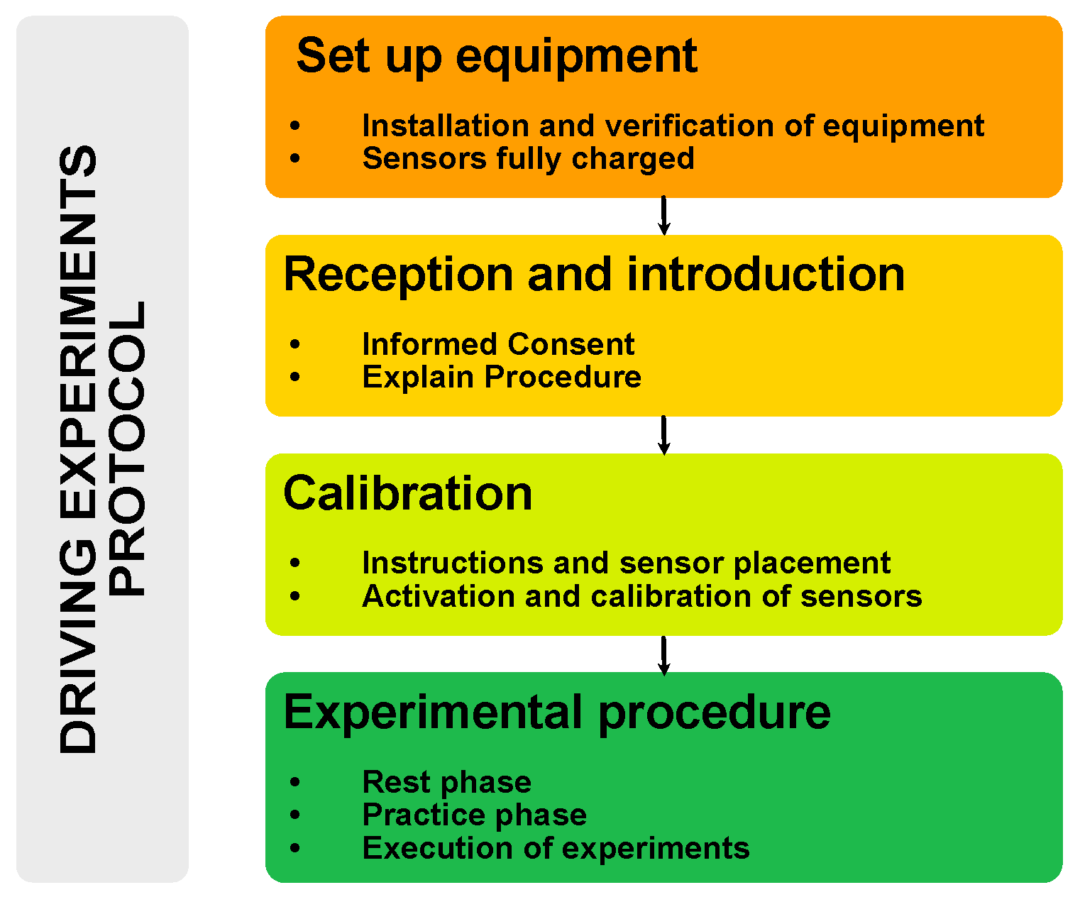
Figure 1. General diagram of the driving experiment protocol.
Electronics 14 04655 g001
Figure 2. Examples of adverse driving events used to trigger takeover requests (TORs).
Electronics 14 04655 g002
Figure 3. Attention level assessment through stimulus detection and gear-shift response. (a) Shifter up. (b) Shifter down.
Electronics 14 04655 g003
Figure 4. Simulation setup general diagram.
Electronics 14 04655 g004
Figure 5. Simulation platform and data acquisition setup used in the experiments.
Electronics 14 04655 g005
Figure 6. Location of devices on the user’s body.
Electronics 14 04655 g006
Figure 7. Driver S 6 reaction times per event and average response of experiment 2.
Electronics 14 04655 g007
Figure 8. Attention score distribution.
Electronics 14 04655 g008
Figure 9. Driver S 6 reaction times per event and average response of experiment 2.
Electronics 14 04655 g009
Figure 10. LSTM architecture model.
Electronics 14 04655 g010
Figure 11. Evaluation of metrics to determine the optimal number of clusters. (a) Inertia for different values of N k . (b) Silhouette score for different values of N k . (c) Stability-based evaluation.
Electronics 14 04655 g011
Figure 12. Comparison of physiological responses between clusters. (a) Distribution of ecg_HRV_MeanNN by cluster. (b) Evolution of eda_mean_scl along the cluster path.
Electronics 14 04655 g012
Figure 13. Confusion matrix. (a) LSTM global before Bayesian optimization. (b) LSTM global after Bayesian optimization. (c) Cluster PP 1 LSTM. (d) Cluster PP 2 LSTM.
Electronics 14 04655 g013
Figure 14. Confidence intervals for global model, Cluster 1 and Cluster 2.
Electronics 14 04655 g014
Figure 15. Cluster-based model performance vs. subject-matched global model performance.
Electronics 14 04655 g015
Figure 16. Model performance comparison with a higher noise level.
Electronics 14 04655 g016
Table 1. Summary of experiments by topology.
Exp.CARLA TownEnvironmentTOR Urgency LevelConcentration LevelScenariosTOR TimeEXP. Time
14Semi-urbanLow/highFocused/distractedAbrupt lane change, pedestrian crossing, obstacle in the road/stopped vehicle 1 21 3 28 4 37 5 16
25UrbanLow/high/criticalFocused/distractedObstruction by stopped vehicle, traffic accident, dynamic obstacle in lane 1 43 3 40   6 00 7 14
Table 2. Features extracted by signal type.
Signal TypeFeature CategoryExtracted Features
ECGHRV–Time DomainMeanNN, SDNN, RMSSD, MedianNN, MadNN, MinNN, MaxNN, pNN50
HRV–Frequency DomainLF, HF, LF/HF ratio
HRV–NonlinearSD1, SD2, SD1/SD2 ratio, Approximate Entropy (ApEn)
EDATonic (SCL)Mean SCL, Max SCL, Min SCL, SCL Slope, SCL Std, Variance, Energy
Phasic (SCR)SCR Count, SCR Rate, Mean Amplitude, Max Amplitude, Amplitude Std
StatisticalMean Diff, Max Diff between successive values
IMU (MetaWear)Raw Motion DataLinear Acceleration (X, Y, Z), Angular Velocity (X, Y, Z), Quaternion (W, X, Y, Z)
Behavioral State LabelHands-on-Wheel binary label (1 = contact, 0 = no contact)
Attention LogsAttentional ScoreCoded values based on visual stimulus (0 = distracted, [0.6–1.0] = semi-distracted, 2 = focused)
Simulator LogsVehicle and Scenario StateSpeed, Control Mode, Planner State, Obstacle Proximity, TOR trigger timestamps
Table 3. Demographic summary statistics by group (General, GR1, GR2).
VariableCategoryGeneral (100%)GR1GR2
FR#%StatsFR#%StatsFR#%Stats
GenderMale (M)1963.31066.7960
Female (F)1136.7533.3640
Age (years)Min--22--23--22
Max--71--71--70
Mean--36--36.33--35.87
Median--33.5--33--34
SD--12.7--12.73--12.62
Driving
Experience
(Years)
Min--0.6--1--0.6
Max--55--50--55
Mean--14.95--14.13--15.77
Median--8.5--7--13
SD--14.33--13.81--14.78
Previous
Autonomous
Driving
Experience
Yes (Y)413.3213.3213.3
No (N)2686.71386.71386.7
FR# = frequency count; Stats = statistical measures (mean, median, min, max, SD).
Table 4. Distribution of attention configuration by group and experiment.
GroupExperimentAttention Configuration
11FOCUSED → DISTRACTED → DISTRACTED (FDD)
2DISTRACTED → FOCUSED → FOCUSED (DFF)
21DISTRACTED → DISTRACTED → FOCUSED (DDF)
2FOCUSED → FOCUSED → DISTRACTED (FFD)
Table 5. ANOVA results showing the most discriminative physiological features ranked by p-value.
Featurep-Value
prediction1.88 × 10 69
eda_energy9.39 × 10 62
ecg_HRV_MinNN2.60 × 10 61
eda_min_scl4.12 × 10 52
eda_max_diff1.00 × 10 51
eda_mean_scl7.41 × 10 47
ecg_HRV_MedianNN1.54 × 10 41
eda_max_scl5.63 × 10 32
ecg_HRV_RMSSD5.75 × 10 23
ecg_HRV_SD19.79 × 10 23
ecg_HRV_HF2.67 × 10 21
ecg_HRV_SD1SD28.28 × 10 21
ecg_HRV_SDNN1.17 × 10 19
eda_mean_diff2.94 × 10 18
ecg_HRV_SD26.26 × 10 17
eda_scr_rate2.20 × 10 15
eda_scr_count2.20 × 10 15
ecg_HRV_MeanNN7.06 × 10 15
ecg_HRV_MaxNN4.81 × 10 13
ecg_HRV_LF2.80 × 10 12
eda_scl_slope1.09 × 10 11
ecg_HRV_ApEn6.18 × 10 6
eda_scl_std3.46 × 10 5
eda_scr_amplitude_mean3.97 × 10 2
eda_variance5.18 × 10 2
ecg_HRV_MadNN1.18 × 10 1
ecg_HRV_LFHF2.11 × 10 1
eda_scr_amplitude_max2.28 × 10 1
eda_scr_amplitude_std4.34 × 10 1
ecg_HRV_pNN508.54 × 10 1
Table 6. Accuracy (%) by feature count.
LSTM24 Features27 Features30 Features
Global95.34%94.50%95.15%
Cluster 175.58%78.47%94.08%
Cluster 268.17%75.05%89.22%
Table 7. Clustering stability and internal validation metrics for different values of K.
KSilhouetteInertiaMean ARINull MeanGapZ-Score
20.1931023.260.6970.00490.6928.66
30.123917.550.4880.00040.4886.62
40.117836.340.4350.00420.4315.52
Table 8. Demographic and physiological experiment 1 and experiment 2 mean summary by cluster.
ClusterSubjectsDemographicecg_HRV_MeanNNeda_mean_scl
AgeGenderExpMeanStdMeanStd
Cluster PP 1S0344M4−51.61±41.510.14±0.27
S0535F20−20.05±25.291.99±0.3
S0742M24−87.08±30.490.63±0.25
S1030M4−136.74±24.981.15±0.15
S1224M7−38.74±13.670.14±0.17
S1333M1−17.34±27.961.52±0.24
S1531F3−91.11±37.763.04±0.36
S1636M19−63.42±44.580.69±0.13
S1822M0.631.16±29.160.71±0.67
S2040M150.62±26.970.39±0.03
S2570M55−36.85±59.780.08±0.19
S1923M7−9.24±28.521.03±0.29
S2924M724.79±29.370.73±0.26
Cluster PP 2S0124M8−9.75±27.64.0±0.64
S0223M7−20.24±28.53.57±0.2
S0449F3377.95±15.424.31±0.31
S0625F11.44±31.643.84±0.5
S0831M11−58.55±18.562.45±0.25
S1135M5−67.06±23.524.24±0.11
S1429M1316.04±44.023.02±0.21
S1725M9−13.65±23.633.3±0.3
S2135F15106.31±74.83.29±0.28
S2256M4020.45±12.053.16±0.47
S2328M7−100.08±36.361.89±0.25
S2430F3−109.87±65.331.23±0.26
S2639F23−8.4±27.522.09±0.28
S2734F1−2.96±20.543.32±0.21
S2871F50−149.21±29.443.18±0.9
S2951F301.85±14.072.75±0.99
S3044F26111.02±292.664.53±0.56
Table 9. Hyperparameter configurations per model.
ParameterGlobalGlobal BOCluster PP 1Cluster PP 2YoungOldMaleFemalePCA 1.1PCA 1.2NoviceExperienced
Window size51513111014591110514
LSTM units64801171271204810211437120101115
Dropout0.30.312780.338880.223430.497520.38150.222980.239950.200320.497520.288910.38473
Fully Connected Layers641148424991231163393994986
Learning rate1.0 × 10 3 5.3 × 10 3 1.0 × 10 2 9.3 × 10 3 4.2 × 10 3 9.8 × 10 3 9.3 × 10 3 9.6 × 10 3 9.1 × 10 3 4.2 × 10 3 8.1 × 10 3 6.5 × 10 3
Table 10. Computational performance comparison between global and cluster-specific LSTM models.
MetricGlobalCluster 1Cluster 2
Total parameters83,44679,40683,446
Model size (KB)325.96310.18325.96
FLOPs per sample2,415,0121,821,6361,772,660
Avg. inference time per sample (ms)0.0990.1040.103
Throughput (samples/s)10,148.19621.59703.3
Disclaimer/Publisher’s Note: The statements, opinions and data contained in all publications are solely those of the individual author(s) and contributor(s) and not of MDPI and/or the editor(s). MDPI and/or the editor(s) disclaim responsibility for any injury to people or property resulting from any ideas, methods, instructions or products referred to in the content.