An Innovative Multi-Scale Feature Fusion Network for Change Detection of Remote Sensing Images

Abstract

Change detection in remote sensing images is crucial for various applications such as military reconnaissance and urban management. However, traditional change detection methods suffer from low accuracy and complex operations. Meanwhile, existing deep learning approaches struggle to fully understand multi-scale semantic information, and thus still face limitations in accuracy and generalization capability. To overcome these limitations, this paper proposed the MSTAN, which consists of a multi-scale Transformer encoder and a decoder centered on a four-layer ASFF module. The four-layer ASFF module dynamically learns spatially adaptive weights to capture multi-scale semantic information. Comparative experiments demonstrate that MSTAN achieves high-precision change detection. Cross-dataset evaluation experiments demonstrate that MSTAN possesses strong generalization ability. Ablation experiments confirm the effectiveness of the four-layer ASFF module in fusing multi-scale features. Complexity analysis quantifies the computational overhead of the four-layer ASFF module. These results highlight MSTAN’s powerful generalization capability and its promising potential for change detection tasks.

1. Introduction

Change detection in remote sensing images aims to identify temporal differences in land cover or surface features by analyzing co-registered images acquired at different times [1,2,3]. This capability is essential for both military and civilian applications: in military reconnaissance, it enables target situational awareness through high-resolution data acquired from platforms such as drones and remote sensing satellites; in civilian applications, it can assist in accomplishing tasks such as environmental monitoring, land management, and urban planning. Due to the diversity of target types and variations in target scale, change detection method is required to be not only highly accurate but also robust and adaptable.

Traditional change detection approaches typically rely on handcrafted features and manual thresholding techniques. Zhou [4] et al. proposed an adaptive threshold selection strategy that incorporates a weighting mechanism to achieve image denoising. He [5] et al. developed a dynamic threshold algorithm based on the fuzzy C-means algorithm, which can better preserve image detail during the denoising process. However, these methods are highly dependent on expert knowledge and sensitive to environmental variations, often yielding inconsistent results in complex scenarios.

In contrast, deep learning-based methods have emerged as promising alternatives due to their strong capabilities in nonlinear expression. Deep learning architectures for change detection are broadly categorized into single-stream and dual-stream models. Single-stream models merge data from two time phases into a single feature space for extraction and classification. Although convolutional neural networks (CNNs) such as UNet++ [6] have been adapted for change detection, their reliance on fixed receptive fields limits their ability to model long-range dependencies.

In contrast, dual-stream models utilize weight-sharing Siamese networks to independently process two temporal images, preserving temporal symmetry and improving feature comparability. The FC-Siam-Diff model [7] computes difference maps through absolute operations in skip connections, enhancing change sensitivity. In recent years, Transformer-based architectures have attracted widespread attention due to their powerful capability in modeling global information. Change detection models based on the Transformer architecture are increasingly emerging. For instance, ChangeFormer [8] effectively captures the multi-scale long-range details required for change detection tasks by leveraging self-attention mechanisms. The Swin Transformer [9] is a variant of the standard Transformer. It effectively addresses the high computational and memory costs of traditional Transformers when processing high-resolution images by introducing a “shifted window” mechanism. As a result, it shows strong potential in remote sensing image change detection, particularly in handling images with complex backgrounds and diverse types of changes. The Swin ResNet Transformer [10] combines the Swin Transformer structure with the ResNet architecture to enhance the ability of model to represent and model multi-scale context. ConvNeXt [11] is an emerging convolutional neural network architecture inspired by Vision Transformers [12]. It retains the classical CNN structure while incorporating improvements in multiple aspects. The Cascaded U-Net model [13] utilizes ConvNeXt to efficiently extract target features, thereby providing stronger feature representation capabilities for change detection tasks. Meanwhile, FCIHMRT [14] adopts a dual-branch feature extraction architecture that combines the strong local feature extraction capability of Res2Net with the advantage of Transformer in capturing long-range dependencies. Feature interaction through cross-layer connections enhances feature extraction capabilities. This method has been effectively applied to remote sensing scene classification tasks. Inspired by this approach, HUTNet [15] employs Unet++ as the backbone to extract multi-scale features and introduces a Transformer-based feature fusion module to capture long-range dependencies, achieving superior performance in change detection.

Despite these advances, existing methods still face critical challenges. On one hand, single-stream models risk information distortion during data fusion, leading to “false changes” and detection errors. On the other hand, dual-stream models, while generally outperforming single-stream models, typically connect or sum difference feature maps directly at the channel level. This approach fails to fully capture multi-scale semantic information, limiting its ability to detect subtle changes, especially in complex and heterogeneous scenes.

To address the above issues, this paper proposes the Multi-Scale Siamese Transformer Adaptive Network (MSTAN). More specifically, the main contributions of this paper are as follows:

(1)

We designed the MSTAN architecture. It integrates a multi-scale Transformer encoder and a decoder centered on a four-layer Adaptive Spatial Feature Fusion (ASFF) module. Among them, the four-layer ASFF module learns spatially adaptive weights for multi-scale features, enabling precise capture of change-sensitive information and effective suppression of background noise.

(2)

We conducted comprehensive comparative experiments on LEVIR-CD and CLCD datasets. The results confirm superior accuracy and robustness over existing methods in complex scenes.

(3)

We conducted cross-dataset evaluation experiments to validate the generalization capability of MSTAN. The results demonstrate that MSTAN outperforms other models across datasets, exhibiting superior generalization ability.

(4)

We conducted ablation experiments to validate the ASFF module. It prove the ASFF module outperforms static concatenate fusion.

(5)

We quantified the computational overhead of the ASFF module through complexity analysis. This provides a clear basis for balancing performance and cost in practical deployment.

We also identified limitations of MSTAN through experiments, ensuring research completeness and guiding future optimization.

2. Methods

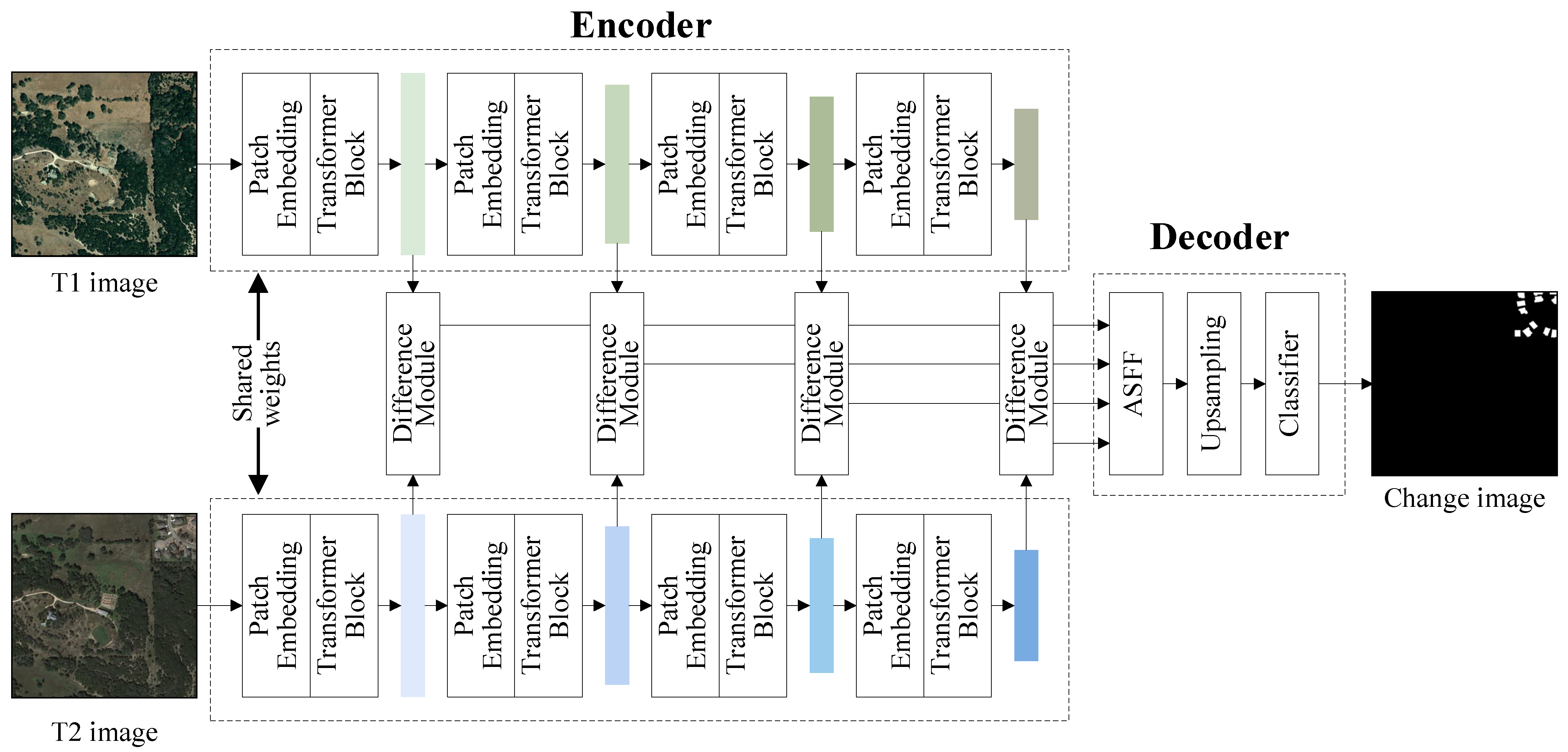
The structure of MSTAN is shown in Figure 1. The model employs a Siamese network architecture, consisting of an encoder and a decoder. The encoder utilizes Transformer blocks to extract multi-scale features from two input images (T1 image and T2 image), while the decoder employs a four-layer Adaptively Spatial Feature Fusion (ASFF) module to integrate these multi-level features and generates the final change detection results.

2.1. Multi-Scale Encoder Based on Transformer

For the given input images (T1 image and T2 image), the multi-scale Transformer encoder generates a sequence of multi-scale features. This process is similar to the hierarchical feature extraction approach of UNet [16], but replaces traditional convolution with Transformer blocks to capture global contextual information. Meanwhile, a sequence reduction strategy is employed within the Transformer blocks to further optimize computational efficiency. Specifically, given input images of size $H\times W\times C$, then the encoder outputs four sets of feature maps $X^l$, each with a resolution of ${\displaystyle \frac{H}{2^{l+1}}}\times {\displaystyle \frac{W}{2^{l+1}}}\times C_l$, where $l=\{1,2,3,4\}$. These multi-level feature maps are subsequently fed into the difference module to compute the change information between the two temporal images.

2.1.1. Patch Embedding

The Patch Embedding module divides the image into equally sized patches and reduces the spatial resolution. The resolution of the output feature map $Ou{t}_{pat}^l$ from the $l$-th layer of this module is ${\displaystyle \frac{H}{2^{l+1}}}\times {\displaystyle \frac{W}{2^{l+1}}}\times C_l$, where $l=\{1,2,3,4\}$. Each downsampled feature map $Ou{t}_{pat}^l$ then fed into the subsequent encoder to obtain feature information at this resolution.

2.1.2. Transformer Block

The Transformer Block in MSTAN is designed to enhance feature extraction from embedded patches. The core of this block is the self-attention mechanism [17], defined as:

$$Attention(Q,K,V)=Softmax({\displaystyle \frac{Q{K}^T}{\sqrt{d_{head}}}})V$$

(1)

where $Q, K$ and $V$ denote query, key, and value matrices, respectively; $d_{head}$ denotes the dimension of the attention head, determining the granularity of local feature interaction.

$Q, K$ and $V$ matrices share the same dimension of $HW\times C$, resulting in a computational complexity of $O({(HW)}^2)$. For high-resolution images, the large number of spatial elements leads to significant computational overhead, which hinders efficient processing. To mitigate this issue, we adopt a sequence reduction process that shortens the sequence length using a reduction ratio $R$, as follows:

$$\begin{array}{l}\tilde{K}=\mathrm{Reshape}\left(HW/R,C·R\right)(K)\\ K^{\prime }=\mathrm{Linear}(C·R,C)(\tilde{K})\end{array}$$

(2)

where $\mathrm{Reshape}\left(H,W\right)$ denotes the reshaping operation on a tensor with the shape of $\left(H,W\right)$; and $\mathrm{Linear}(C_1,C_2)$ denotes a linear layer with input channel dimension $C_1$, output channel dimension $C_2$; $R$ is the reduction ratio.

Following this reduction strategy, the size of the $K$ matrix is reduced to $\left(HW/R,C\right)$. Similarly, applying the same operation to the $Q$ and $V$ matrices, the computational complexity is reduced to $O({(HW)}^2/R)$.

2.1.3. Difference Module

The Difference Module computes the feature differences across multiple levels generated by the dual-branch Transformer encoder. Specifically, the feature maps from the two shared encoder branches are concatenated along the channel dimension. The resulting tensor is then processed through a series of convolutional layers followed by BatchNorm and ReLU activation functions, expressed as:

$$X_{diff}^l=ReLU(Con{v}_{3\times 3}(BN(ReLU(Con{v}_{3\times 3}(Cat(X_1^l,X_2^l))))))$$

(3)

where $X_1^l$ and $X_2^l$ denote encoded features corresponding to images before and after changes at the $l$-th layer; $Con{v}_{3\times 3}$ denotes convolution operation with a 3 × 3 convolution kernel; $Cat(\cdot )$ denotes channel-wise tensor concatenation; the concatenation operation is chosen to preserve the complete numerical values and relative relationships of the two features as in [8], thereby enhancing the model’s ability to represent change patterns.

2.2. Decoder Based on Multi-Scale Adaptive Fusion

The encoded multi-scale features are decoded through a four-layer ASFF module, followed by upsampling and a classification layer, to generate the final binary change map. The output is resized to the original input resolution and converted to two channels, producing an output of size $H\times W\times 2$.

2.2.1. Four-Layer ASFF

The four-layer ASFF module is designed to improve the fusion effect of multi-scale difference features by adaptively learning spatial fusion weights. This adaptive feature fusion method can dynamically adjust the weights of features at different scales according to the input feature set, integrate deep semantics and shallow details, thereby effectively utilizing multi-scale information. It enables the network to maintain continuous and consistent representations of the target’s multi-scale variations, improving the model’s expressive ability and generalization performance, and thus enhancing the performance of change detection, thereby improving the performance of change detection.

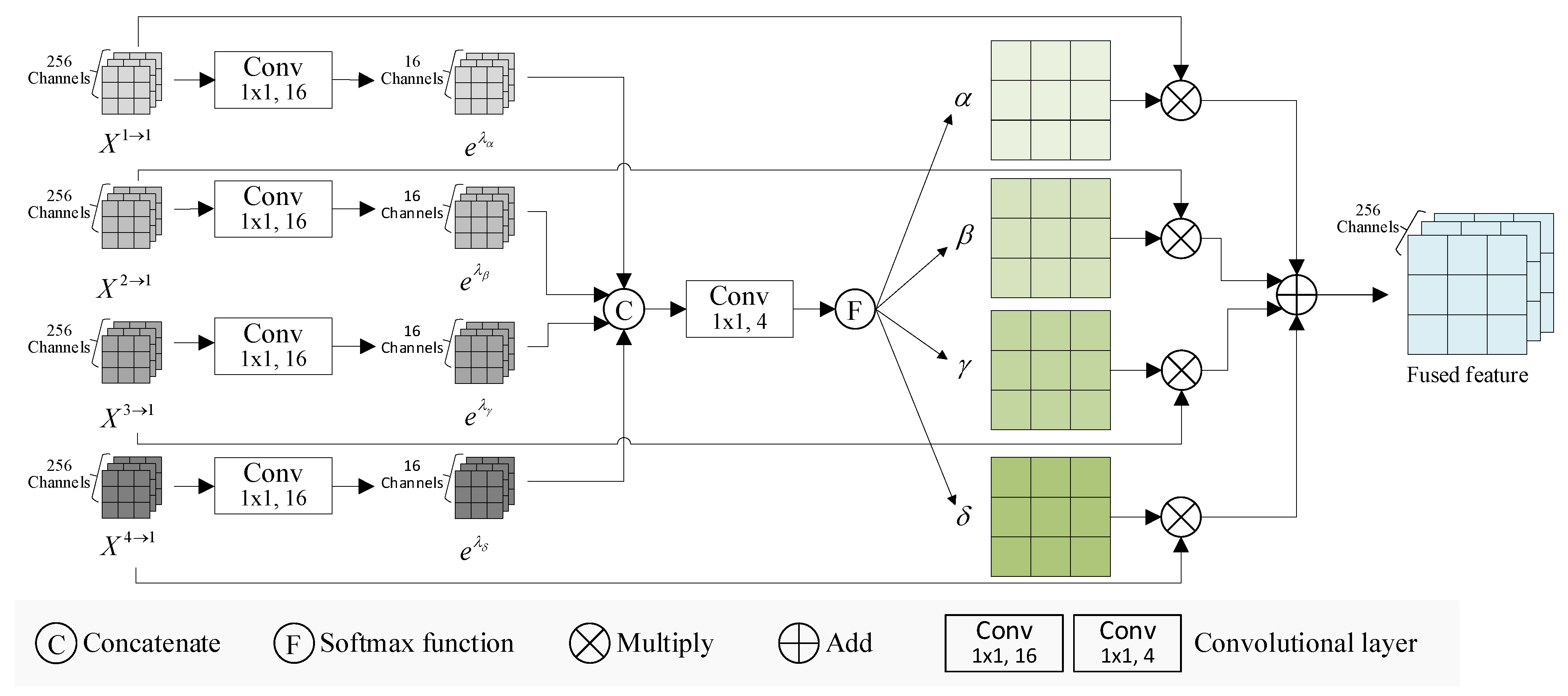
The structure diagram of the Four-layer ASFF module is shown in Figure 2. The fusion process consists of two steps:

(1)

Scale Alignment: Features from all levels are upsampled to match the spatial resolution of the finest-level (level-1) feature map. Specifically, since the resolution of the multi-level feature maps output from the encoder is ${\displaystyle \frac{H}{2^{l+1}}}\times {\displaystyle \frac{W}{2^{l+1}}}\times C_l$, where $l=\{1,2,3,4\}$, the level-4 feature map is upsampled by a factor of 8 to obtain $X^{4\to 1}$, the level-3 feature map is upsampled by a factor of 4 to obtain $X^{3\to 1}$; the level-2 feature map is upsampled by a factor of 2 to obtain $X^{2\to 1}$; while level-1 remains unchanged, resulting in $X^{1\to 1}$.

(2)

Adaptive Fusion: At each spatial position $(i,j)$, the fused feature is computed as a weighted sum of the aligned feature vectors from all four levels. The weights are learned adaptively through a learnable mechanism, with all channels sharing the same spatial weights. The fusion is formulated as:

$$Y_{ij}={\alpha }_{ij}\cdot X_{ij}^{1\to 1}+{\beta }_{ij}\cdot X_{ij}^{2\to 1}+{\gamma }_{ij}\cdot X_{ij}^{3\to 1}+{\delta }_{ij}\cdot X_{ij}^{4\to 1}$$

(4)

where ${\alpha }_{ij},{\beta }_{ij},{\gamma }_{ij}$ and ${\delta }_{ij}$ denote the fusion weights assigned to the feature maps at four levels at the pixel spatial location $(i,j)$, and these weight values can be computed through Equation (5).

$$\begin{array}{l}{\alpha }_{ij}={\displaystyle \frac{e^{{\lambda }_{{\alpha }_{ij}}}}{e^{{\lambda }_{{\alpha }_{ij}}}+e^{{\lambda }_{{\beta }_{ij}}}+e^{{\lambda }_{{\gamma }_{ij}}}+e^{{\lambda }_{{\delta }_{ij}}}}}\\ {\beta }_{ij}={\displaystyle \frac{e^{{\lambda }_{{\beta }_{ij}}}}{e^{{\lambda }_{{\alpha }_{ij}}}+e^{{\lambda }_{{\beta }_{ij}}}+e^{{\lambda }_{{\gamma }_{ij}}}+e^{{\lambda }_{{\delta }_{ij}}}}}\\ {\gamma }_{ij}={\displaystyle \frac{e^{{\lambda }_{{\gamma }_{ij}}}}{e^{{\lambda }_{{\alpha }_{ij}}}+e^{{\lambda }_{{\beta }_{ij}}}+e^{{\lambda }_{{\gamma }_{ij}}}+e^{{\lambda }_{{\delta }_{ij}}}}}\\ {\delta }_{ij}={\displaystyle \frac{e^{{\lambda }_{{\delta }_{ij}}}}{e^{{\lambda }_{{\alpha }_{ij}}}+e^{{\lambda }_{{\beta }_{ij}}}+e^{{\lambda }_{{\gamma }_{ij}}}+e^{{\lambda }_{{\delta }_{ij}}}}}\end{array}$$

(5)

where the weight scalar mappings ${\lambda }_{{\alpha }_{ij}}, {\lambda }_{{\beta }_{ij}}, {\lambda }_{{\gamma }_{ij}}$ and ${\lambda }_{{\delta }_{ij}}$ are obtained by applying a 1 × 1 convolutional layer to the scaled feature map $X_{ij}^{1\to 1}, X_{ij}^{2\to 1}, X_{ij}^{3\to 1}$ and $X^{4\to 1}$, enabling the network to adaptively learn information from different feature maps through the backpropagation mechanism.

At the same time, these weights are constrained by Equation (6). We can implement this constraint using the softmax function.

$${\alpha }_{ij}+{\beta }_{ij}+{\gamma }_{ij}+{\delta }_{ij}=1,{\alpha }_{ij},{\beta }_{ij},{\gamma }_{ij},{\delta }_{ij}\in [0,1]$$

(6)

The detailed process of adaptive fusion is shown in Figure 3.

Remote sensing images exhibit inherent non-uniform multi-scale semantic distributions, due to varying land cover types and target scales within scenes. This fundamental difference in multi-scale features creates significant challenges to static fusion methods (e.g., concatenation or fixed-weight summation). These approaches treat multi-scale features as equally important across the entire spatial domain, assigning equal channel weights to low-level and high-level features without accounting for the weight values required for different targets. Consequently, in areas with small targets, boundary detection becomes blurred due to the involvement of high-level semantic features. Conversely, in areas with large targets, fusion features are diluted by low-level noise, diminishing semantic discrimination capabilities.

In contrast, the four-layer ASFF module theoretically resolves this mismatch issue. By learning spatially adaptive weights, it dynamically assigns more appropriate weights to corresponding features at each spatial location.

2.2.2. Upsampling and Classifier

Upsampling restores the fused feature map to the original input resolution. Each upsampling step doubles the spatial dimensions and is implemented using a transposed convolution operation. To mitigate performance degradation associated with deep network architectures, a residual connection is incorporated, expressed as:

$$\mathrm{Residual}(X)={\mathrm{Conv}}_{3\times 3}(\mathrm{ReLU}({\mathrm{Conv}}_{3\times 3}(X)))+X$$

(7)

where $X$ denotes the input features, which specifically refers to the feature fused by the four-layer ASFF module.

Thus, Upsampling can is expressed as:

$$X_{ups}=\mathrm{Residual}(\mathrm{ConvTranspose}(X))$$

(8)

where $\mathrm{ConvTranspose}(\cdot )$ denotes the transposed convolution operation, $\mathrm{Residual}(\cdot )$ denotes the residual connection as in Equation (7).

Finally, a linear layer with an output dimension of 2 is used as the classifier to produce binary change detection results.

3. Results and Discussion

In this section, we present the experimental setup, along with the corresponding results and discussions. Specifically, we detail the datasets used, the implementation specifics. Subsequently, the performance of the MSTAN model is evaluated and compared with existing approaches to demonstrate its effectiveness and generalization. Meanwhile, ablation experiments and complexity analysis of the four-layer ASFF module were conducted to demonstrate its effectiveness.

3.1. Experimental Setup

3.1.1. Implementation Details

The proposed model was implemented in Python 3.8 using PyTorch 1.10.1 and trained on an NVIDIA GeForce RTX 3090 GPU. Partial architectural details of MSTAN are shown in

Table 1. Partial architecture details of MSTAN.

Layer Number	Patch Embedding	Transformer Block		Difference Module
	Embedding Dimensions	Number Heads	Stacking Numbers	Output Dimensions
1	64	1	3	256
2	128	2	3	256
3	320	4	4	256
4	512	8	3	256

In the table, “Layer number” denotes the hierarchical level index of the encoder, “Number heads” denotes the number of heads in the Transformer multi-head attention mechanism, and “Stacking number” denotes the number of stacked Transformer blocks.

, and we initialized the network parameters randomly.

The AdamW optimizer was used for network optimization with the following parameter settings: initial learning rate of 0.0001, first-order momentum decay coefficient ${\beta }_1$ of 0.9, second-order momentum decay coefficient ${\beta }_2$ of 0.999, and weight decay coefficient of 0.01. The batch size was set to 16, and the network was trained for 400 epochs using the Cross-Entropy (CE) loss function. During training, each epoch was followed by validation on the validation dataset. After training, we evaluated the model on the test dataset and reported the scores of the relevant metrics.

3.1.2. Datasets

Experiments were conducted on two publicly available datasets: LEVIR-CD [18] and CLCD [19]. Specifically, the LEVIR-CD dataset, primarily designed for building change detection, contains 637 image pairs of 1024 × 1024 pixels, covering various architectural targets such as residences, small garages, and large warehouses. The CLCD dataset, mainly used for farmland change detection, includes 600 image pairs of 512 × 512 pixels, encompassing multiple target types like buildings, roads, lakes, and bare land.

The data augmentation strategies adopted in this paper for the two datasets are as follows:

(1)

All images are resized to 256 × 256 pixels using linear interpolation;

(2)

Horizontal and vertical flipping are applied with a probability of 50% to simulate mirror symmetry and increase data diversity;

(3)

Random rotations of 90°, 180°, or 270° are performed with a probability of 50% to enhance the robustness of model to angular variations;

(4)

A 1:1 aspect ratio crop region is randomly selected with a scaling factor between 0.8 and 1.2 to simulate varying shooting distances and viewpoints;

(5)

Random scaling between 1.0× and 1.2× is applied, followed by random cropping to the target size, enabling more flexible scale variations;

(6)

Gaussian blur is randomly applied to simulate out-of-focus or motion blur effects;

(7)

Brightness, contrast, saturation, and hue are randomly adjusted within a ±30% range to improve the robustness of model to illumination changes.

3.2. Comparative Experiments

To evaluate the performance of the proposed model in change detection, comprehensive comparative experiments were conducted on the LEVIR-CD and CLCD datasets. The method was compared with several approaches: FC-EF [7], FC-Siam-Di [7], FC-Siam-Conc [7], DTCDSCN [20], BIT [21], and RDP [22]. Below is a brief introduction to these models:

FC-EF: employs a Fully ConvNet to process concatenated bitemporal images for change detection.

FC-Siam-Di: utilizes a Siamese Fully ConvNet to extract multi-level features and detect changes through feature differences.

FC-Siam-Conc: also based on a Siamese Fully ConvNet, detects changes by concatenating multi-level features. These fully convolutional network models have surpassed the state-of-the-art change detection methods (2018) in both accuracy and inference speed for change detection as described in [7].

DTCDSCN: leverages a dual attention module to exploit channel and spatial interdependencies of ConvNet features for change detection. On the WHU building dataset, it has surpassed the state-of-the-art change detection methods (2022) as described in [20].

BIT: employs a simple CNN backbone to extract paired feature maps, and innovatively designs a bi-temporal image Transformer to efficiently model contextual information within the spatio-temporal domain. On three change detection datasets, it has surpassed several state-of-the-art change detection methods (2022) as described in [21].

RDP: utilizes a dual pyramid architecture with residual connections to capture multi-scale features, enhancing change detection through oriented pooling. It has achieved the state-of-the-art empirical performance (2022) as described in [22].

Performance was assessed using five standard metrics: Accuracy, IoU, F1-Score, Precision, and Recall. The evaluation results of different methods on LEVIR-CD and CLCD datasets are shown in

Table 2. The evaluation results of different methods on LEVIR-CD.

Model Name	Accuracy	IoU	F1-Score	Precision	Recall
FC-EF	97.408	76.839	85.365	89.018	82.404
FC-Siam-Di	97.438	76.288	84.906	90.726	80.673
FC-Siam-Conc	97.862	81.066	88.594	89.864	87.412
DTCDSCN	97.960	81.971	89.246	90.043	88.485
BIT	97.858	81.625	89.006	88.731	89.286
RDP	97.229	76.276	84.931	86.854	83.223
MSTAN (Ours)	98.046	82.088	89.321	91.720	87.213

All values in the above table are displayed as percentages. All metric results are the average values obtained from multiple repeated trials. Red bold indicates first place, blue bold indicates second place, and purple bold indicates third place.

and

Table 3. The evaluation results of different methods on CLCD.

Model Name	Accuracy	IoU	F1-Score	Precision	Recall
FC-EF	93.543	55.267	62.895	86.594	58.748
FC-Siam-Di	91.105	47.963	52.297	56.040	52.023
FC-Siam-Conc	92.470	55.744	64.082	71.461	60.975
DTCDSCN	94.088	66.661	76.714	79.275	74.648
BIT	95.001	69.587	79.402	84.208	75.965
RDP	94.016	66.026	76.072	79.128	73.706
MSTAN (Ours)	94.764	70.262	80.101	81.611	78.757

All values in the above table are displayed as percentages. All metric results are the average values obtained from multiple repeated trials. Red bold indicates first place, blue bold indicates second place, and purple bold indicates third place.

, respectively.

On the LEVIR-CD dataset, MSTAN achieves the highest performance in Accuracy (98.046%), IoU (82.088%), F1-score (89.321%), and Precision (91.720%), while ranking fourth in Recall (87.213%). The relatively lower Recall means that there is a certain degree of missed detection for some change areas. The F1—score, which balances Precision and Recall, indicates the overall effectiveness of change detection. The superior F1—score of MSTAN shows that the model can accurately identify change areas in general.

On the CLCD dataset, MSTAN achieves the best results in IoU (70.262%), F1-score (80.101%), and Recall (78.757%), demonstrating strong sensitivity and low omission rates. Although FC-EF achieves the highest score in the Precision (86.594%), its performance on other metrics is relatively low, especially for IoU (55.267%) and Recall (58.748%). This indicates that the model has a high rate of missed detections and low agreement with the ground truth. Clearly, it is not suitable for precise change detection tasks. Although Accuracy (94.764%) and Precision (81.611%) are lower than BIT, MSTAN achieves highter Recall metric compared to the BIT model, and its F1-score also surpasses that of the BIT model. It indicates that MSTAN possesses better generalization capability and robustness.

Overall, MSTAN exhibits consistent and robust performance across both datasets, reflecting strong generalization, stability, and accuracy. The performance advantage of MSTAN stems from the multi-scale Transformer encoder and the four-layer ASFF module. The multi-scale Transformer encoder captures hierarchical features across spatial scales. The adaptive learning mechanism and dynamic weight adjustment strategy of the four-layer ASFF enhance the model’s representation capability for various types of targets (e.g., building targets on LEVIR-CD dataset and farmland targets on CLCD), thereby improving the model’s generalization and robustness, leading to superior overall performance on both datasets.

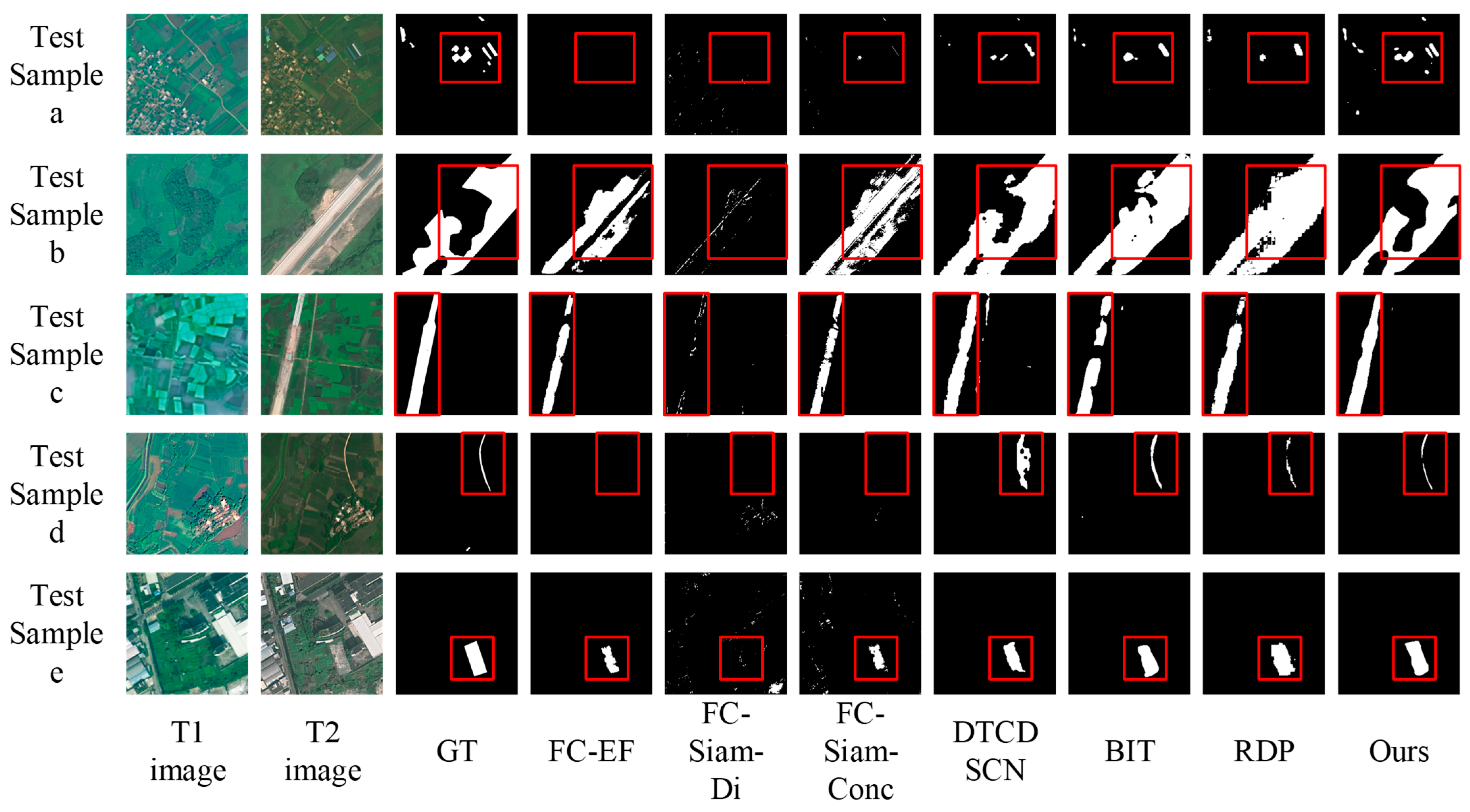
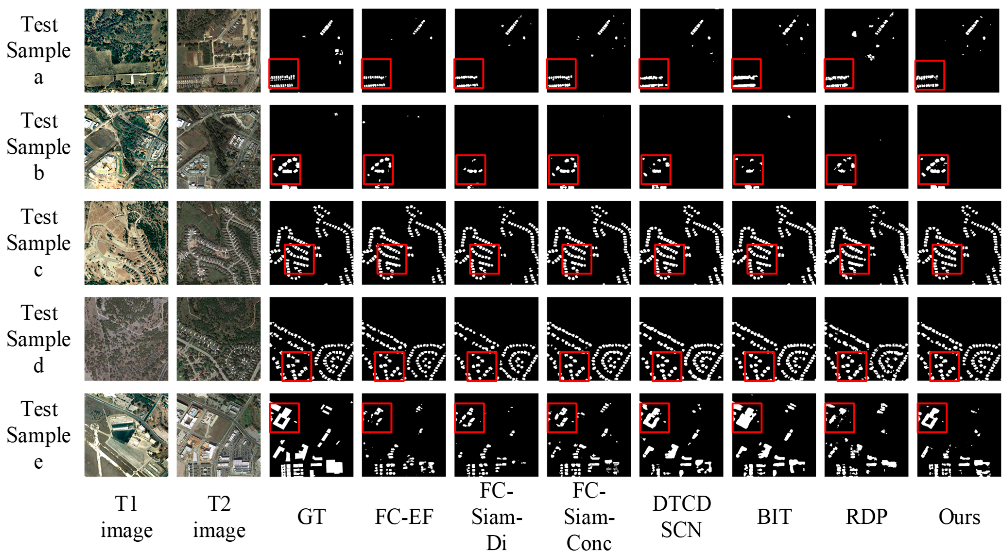
To visually demonstrate the effectiveness of different models in extracting change areas, the visual detection comparisons of various methods on LEVIR-CD dataset are provided in Figure 4.

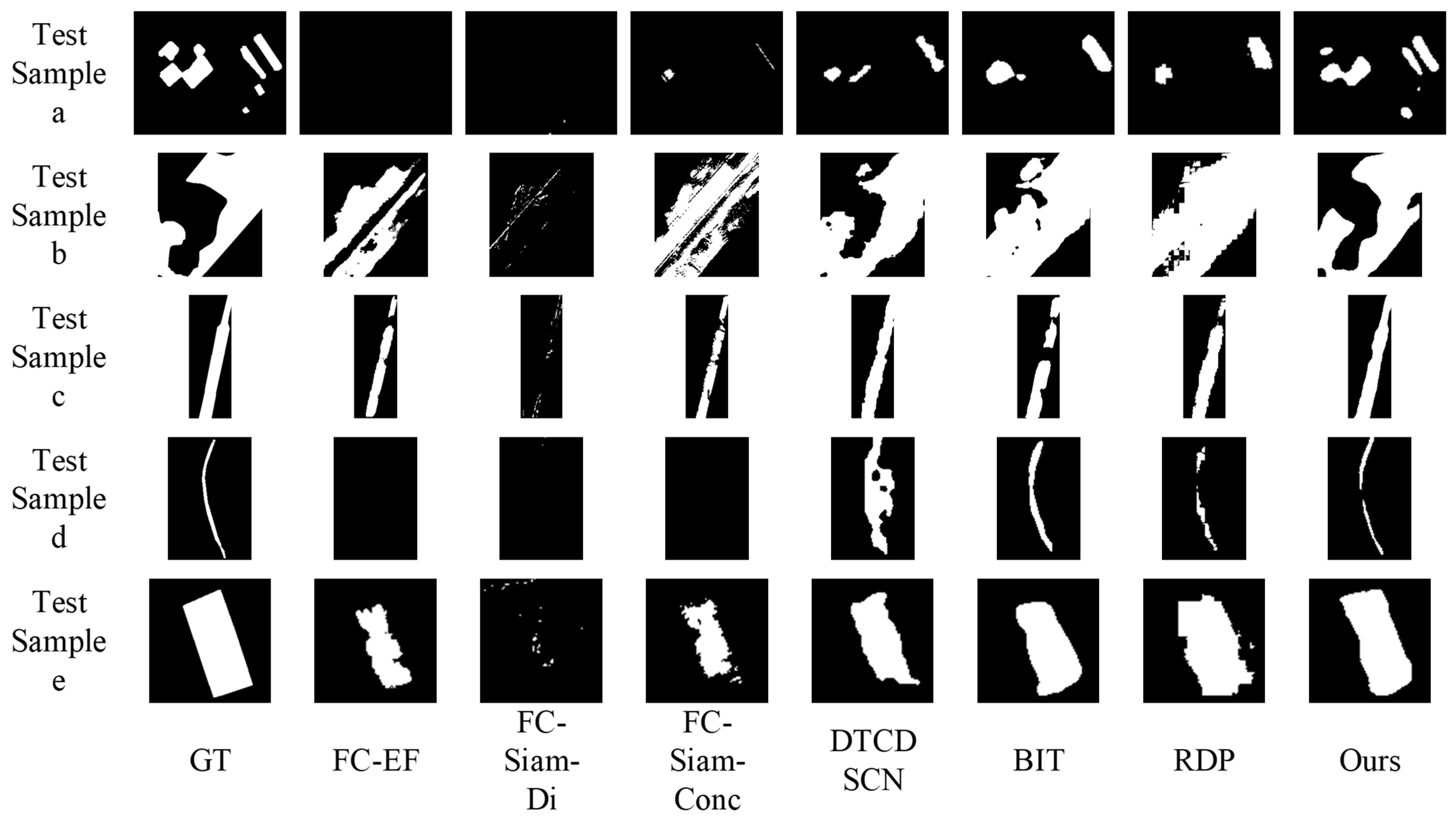
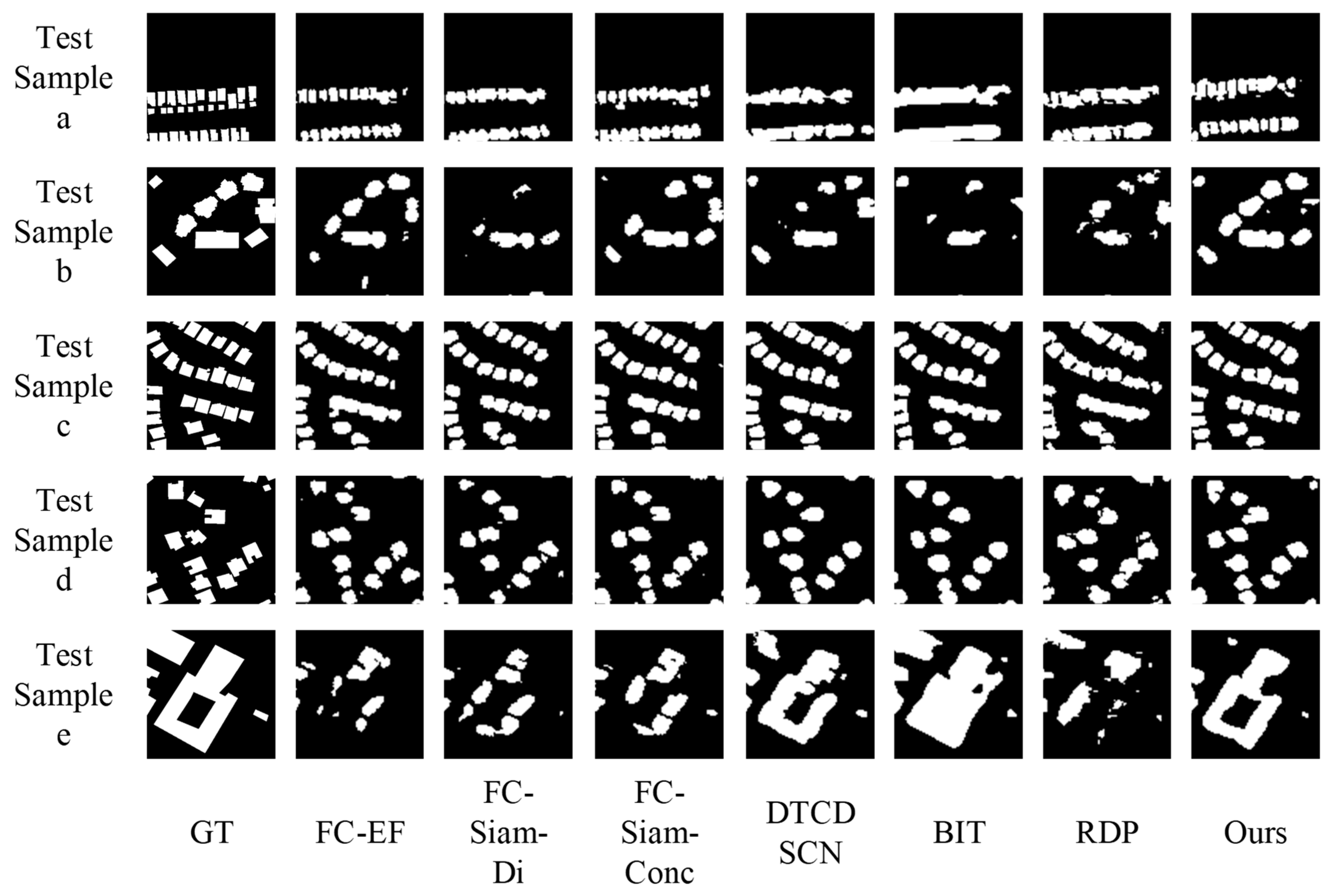
Figure 4. Change detection results of different methods on LEVIR-CD. The regions marked by red rectangles are the pixel areas of interest. The more detailed texture information of this area is shown in Figure 5.

Figure 4. Change detection results of different methods on LEVIR-CD. The regions marked by red rectangles are the pixel areas of interest. The more detailed texture information of this area is shown in Figure 5.

In the figure, each row corresponds to a test sample. The first and second columns show the T1 and T2 images, respectively, while the third column displays the ground truth. Subsequent columns present the change detection maps produced by FC-EF, FC-Siam-Di, FC-Siam-Conc, DTCDSCN, BIT, RDP, and the proposed MSTAN model.

On the LEVIR-CD dataset, as shown in Figure 4, all models detect major changes (e.g., test sample c,d), but differ in detail preservation. FC-EF, FC-Siam-Di, FC-Siam-Conc and RDP exhibit notable edge degradation and missed detections (e.g., test sample b,e). This is consistent with their lower Recall scores. In this regard, BIT captures a larger number of changed areas, but suffers from false alarms (e.g., test samples a,e), which is consistent with its lower Precision score. DTCDSCN shows inferior boundary delineation compared to MSTAN (e.g., test samples b,a). Although MSTAN can accurately detect most of the changed areas, it exhibits a certain number of missed detections compared to models such as BIT (e.g., test sample e), which directly reflects its relatively low Recall score on this dataset.

Figure 5. Detail texture display of interesting regions on LEVIR-CD.

Figure 5. Detail texture display of interesting regions on LEVIR-CD.

The visual detection comparisons of various methods on CLCD dataset are provid-ed in Figure 6. The FC-EF, FC-Siam-Di, and FC-Siam-Conc models exhibit a significant drop in precision and a notable increase in missed detections (e.g., test samples a, d, and e). The RDP, BIT, and DTCDSCN models suffer from severe false and missed detections. In contrast, MSTAN shows a marked improvement in reducing missed detections (e.g., test samples b and c), which corresponds to its higher Recall value. However, it also causes some missed detections (e.g., test samples e), which corresponds to its lower Precision value.

Figure 6. Change detection results of different methods on CLCD. The models and test samples shown in this figure are the same as those in Figure 4. The regions marked by red rectangles are the pixel areas of interest. The detailed texture information of this area in this figure is shown in Figure 7.

Figure 6. Change detection results of different methods on CLCD. The models and test samples shown in this figure are the same as those in Figure 4. The regions marked by red rectangles are the pixel areas of interest. The detailed texture information of this area in this figure is shown in Figure 7.

Figure 7. Detail texture display of interesting regions on CLCD.

Figure 7. Detail texture display of interesting regions on CLCD.

In summary, the above comparative analysis shows that MSTAN exhibits more balanced performance metrics and superior generalization capability across the two datasets. Despite the superior performance of MSTAN in most scenarios, it still has certain limitations.

In terms of handling extremely subtle changes, such as tiny alterations in vegetation coverage on the LEVIR—CD dataset, MSTAN may occasionally miss some of these minute changes. It may limit the model’s applicability in certain sensitive target perception tasks. This is because the four-layer ASFF module, while excellent at fusing multi—scale features for prominent changes, might not be sufficiently sensitive to such extremely fine—grained variations, which can lead to a slight decrease in recall for these specific cases.

When dealing with large—scale, complex scene changes on the CLCD dataset, MSTAN might have difficulty in accurately distinguishing and segmenting each individual object. The adaptive fusion of the four-layer ASFF module, in such highly complex and ambiguous situations, may not always assign the most optimal weights to different scale features, resulting in some inaccuracies in the detailed boundaries of change regions.

3.3. Cross-Dataset Evaluation

To further validate the generalization capability of MSTAN, particularly its universality for two distinct target types: building changes in the LEVIR-CD dataset and cropland changes in the CLCD dataset. We merge the two datasets into a unified data source and unify the training. This approach exposes the training process to varying target scales, thereby reducing the dependence of the model on the statistical characteristics of a single scene.

We use the same standard metrics and comparison models in Section 3.2, and the comparison results of cross-dataset evaluation are shown in

Table 4. Cross-dataset evaluation comparison results of different methods.

Model Name	Accuracy	IoU	F1-Score	Precision	Recall
FC-EF	93.770	46.885	48.392	46.885	50.000
FC-Siam-Di	93.767	46.887	48.398	52.616	50.002
FC-Siam-Conc	93.769	46.889	48.401	62.857	50.004
DTCDSCN	95.387	69.351	79.082	80.955	77.458
BIT	95.586	67.661	77.341	84.523	72.896
RDP	94.904	64.806	74.499	79.739	71.028
MSTAN (Ours)	96.161	72.905	82.227	85.168	79.806

All values in the above table are displayed as percentages. All metric results are the average values obtained from multiple repeated trials. Red bold indicates first place, blue bold indicates second place, and purple bold indicates third place.

.

Experimental results demonstrate that MSTAN achieves the best performance across all evaluation metrics, with Accuracy, IoU, F1-score, Precision, and Recall reaching 96.161%, 72.905%, 82.227%, 85.168%, and 79.806%, respectively. This indicates its outstanding adaptability to diverse scenarios. Detailed analysis reveals that F1-score of MSTAN surpasses the second-ranked model DTCDSCN by 3.145%, precision by 0.645% over the second-ranked model BIT, and recall by 2.348% over the second-ranked model DTCDSCN. This demonstrates its overall robust performance in change detection tasks and superior control over misclassifications and missed detections. The IoU is improved by 3.554% compared to the second-ranked model BIT, indicating that predictions of MSTAN exhibit higher overlap with GT labels and greater accuracy in locating change region boundaries. In contrast, models such as RDP, FC-Siam-Conc, FC-Siam-Di, and FC-EF performed poorly across the board.

Comparing these results with the single-dataset test results on LEVIR-CD in Table 1, it can be seen that MSTAN exhibits a certain degree of decline in some metrics during cross-dataset experiments. For instance, its F1 score on the LEVIR-CD single dataset (89.321%) is significantly higher than the cross-dataset test result (82.227%). Conversely, all metrics for MSTAN improved in the CLCD single-dataset test results shown in Table 2. This indicates that while MSTAN demonstrates exceptional generalization capabilities, there remains room for improvement in handling the compound complexity of multiple datasets. Furthermore, similar trends were observed in other comparison models, where certain metrics in cross-dataset experiments fell below their respective single-dataset test results.

Overall, MSTAN stands out with optimal generalization performance, yet all models face challenges in maintaining consistent performance when handling datasets with significant variations in data distribution.

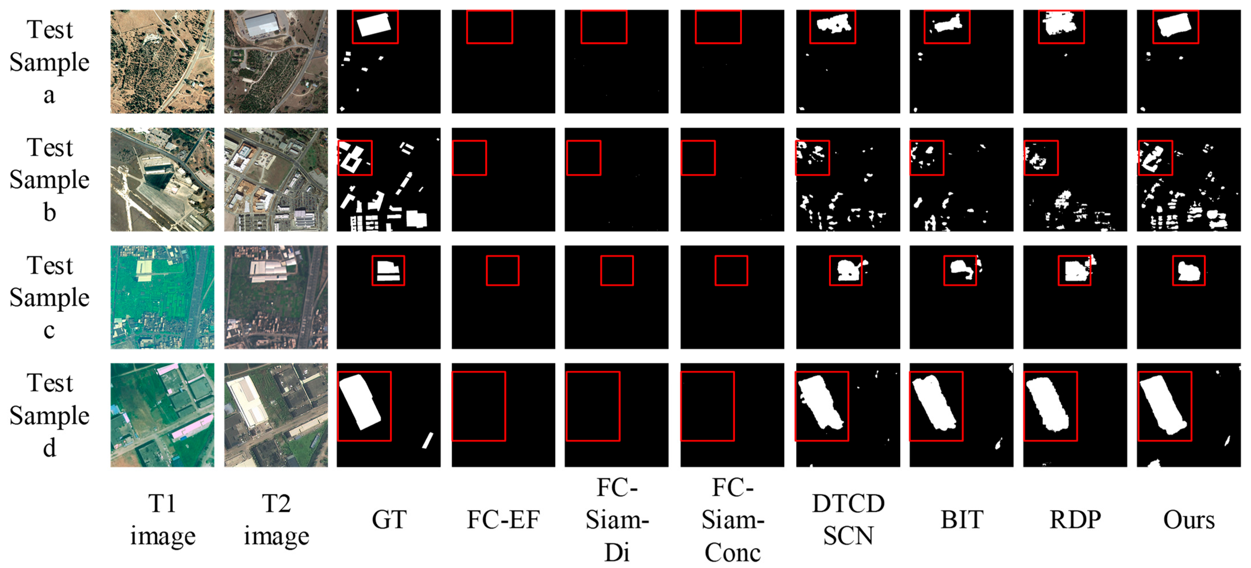
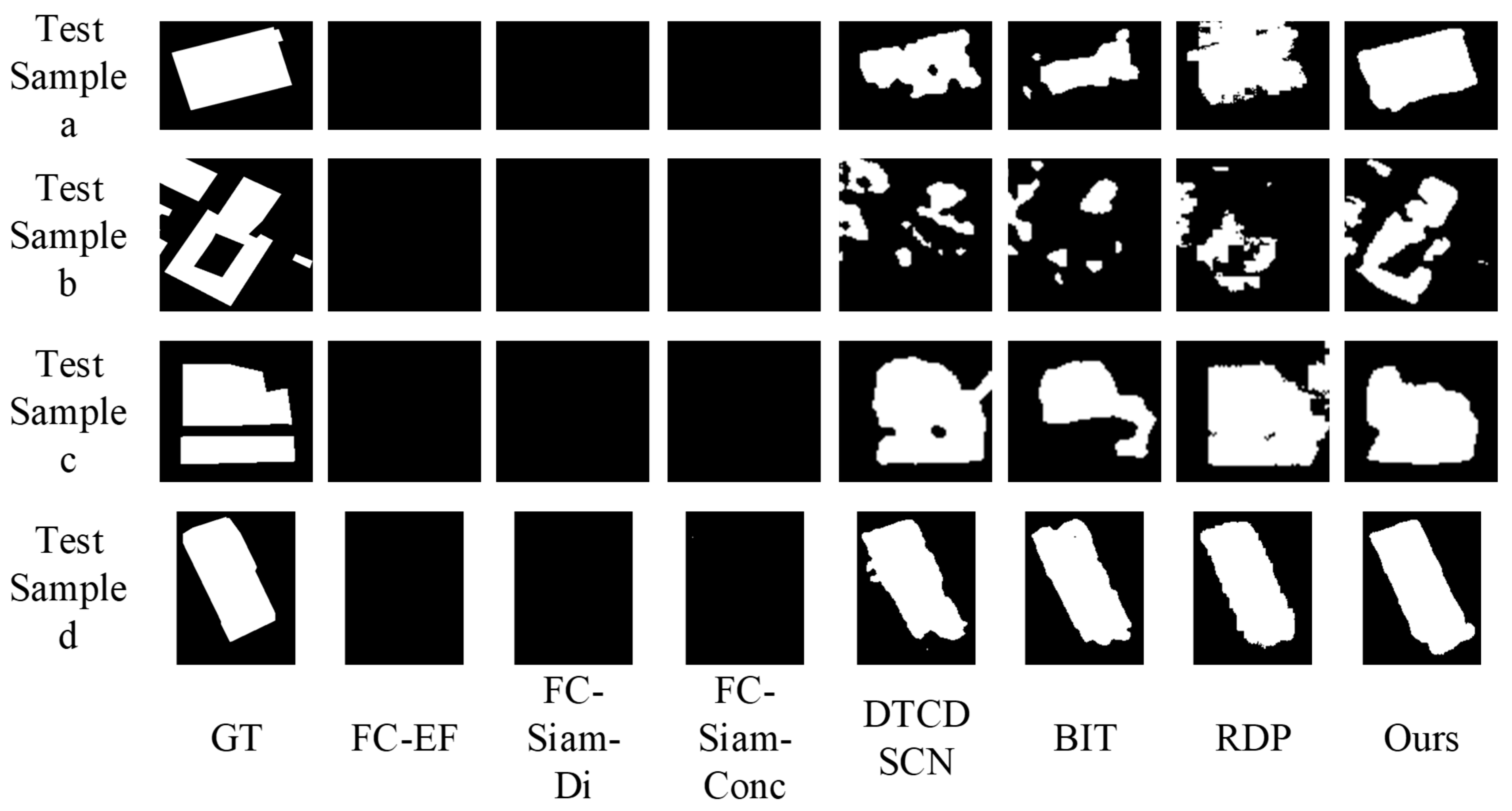
To visually demonstrate the generalization of different models in extracting change areas, the visual detection comparisons of various methods on cross-datasets are provided in Figure 8.

Figure 8. Change detection results of different methods on cross-dataset. The regions marked by red rectangles are the pixel areas of interest. The more detailed texture information of this area is shown in Figure 9.

Figure 8. Change detection results of different methods on cross-dataset. The regions marked by red rectangles are the pixel areas of interest. The more detailed texture information of this area is shown in Figure 9.

In the figure, the first two rows of test samples are from LEVIR-CD dataset, while the last two rows are from CLCD dataset. The first and second columns show the T1 and T2 images, respectively, while the third column displays the ground truth. Subsequent columns present the change detection maps produced by FC-EF, FC-Siam-Di, FC-Siam-Conc, DTCDSCN, BIT, RDP, and the proposed MSTAN model.

As shown in the figure, the FC-EF, FC-Siam-Di, and FC-Siam-Conc models performed poorly overall, detecting almost no regions of change. This represents a significant deviation from single-dataset test results, indicating weak cross-dataset generalization capabilities. The RDP model exhibits numerous false-positive regions (e.g., test samples a, c), corroborating its low Precision metric in Table 4. The BIT and DTCDSCN models demonstrate significant false-negative regions (e.g., test samples a, b), confirming their low Recall scores. In contrast, the MSTAN model exhibits high spatial agreement with GT, demonstrating strong adaptability and accuracy across complex and diverse variation scenarios. This indicates its robust generalization capability and resilience. Its performance advantage likely stems from t adaptive learning strategy of four-layer ASFF module, which effectively learns cross-dataset generalized features. This enhances the target representation capability of model and improves variation detection performance. However, MSATN exhibits suboptimal edge detail representation (e.g., test samples b, c), indicating its shallow-layer information is inadequately captured. This deficiency in edge detail characterization suggests the model struggles to effectively capture or utilize shallow-layer features.

Furthermore, compared to the test results from the single dataset in Figure 4 and Figure 6, a certain degree of decline in detection performance can be observed across all models (e.g., test sample b). This indicates that the generalization capability of MSTAN still has room for improvement.

3.4. Ablation Experiments

To validate the effectiveness of the four-layer ASFF module in change detection tasks, this section conducts comparative ablation experiments on the LEVIR-CD and CLCD datasets. The models compared include MSTAN and MSTAN-C, where MSTAN employs the four-layer ASFF module for multi-scale feature fusion, while MSTAN-C uses the concatenate operation to fuse multi-scale features following the approach in [8]. The comparison results are shown in

Table 5. Ablation experiments results on LEVIR-CD.

Model Name	Accuracy	IoU	F1-Score	Precision	Recall
MSTAN-C	97.955	81.408	88.835	91.173	86.777
MSTAN	98.046 (+0.091)	82.088 (+0.680)	89.321 (+0.486)	91.720 (+0.547)	87.213 (+0.436)

All values in the above table are displayed as percentages. All metric results are the average values obtained from multiple repeated trials. Values highlighted in bold red font indicate the incremental differences in model performance metrics.

and

Table 6. Ablation experiments results on CLCD.

Model Name	Accuracy	IoU	F1-Score	Precision	Recall
MSTAN-C	94.245	68.589	78.614	79.315	77.954
MSTAN	94.764 (+0.519)	70.262 (+1.673)	80.101 (+1.487)	81.611 (+2.296)	78.757 (+0.803)

All values in the above table are displayed as percentages. All metric results are the average values obtained from multiple repeated trials. Values highlighted in bold red font indicate the incremental differences in model performance metrics.

.

On the LEVIR-CD dataset, MSTAN shows improvements across all evaluation metrics, with an IoU increase of 0.680 and an F1-score improvement of 0.486, indicating that the model can more accurately predict changed regions overall, thereby helping to reduce false alarms and missed detections in practical applications.

On the CLCD dataset, MSTAN also demonstrates superior performance, achieving an IoU improvement of 1.673, an F1-score increase of 1.487, and a precision gain of 2.296. A possible reason is that differences in target representation between the LEVIR-CD and CLCD datasets make the traditional concatenate fusion mechanism less effective in learning multi-scale target features. For instance, the two datasets differ in terms of target types, scale sizes, and scale ranges. In contrast, the four-layer ASFF module’s adaptive feature learning and dynamic fusion strategy enable the model to effectively learn more generalizable feature representations, thereby enhancing its generalization capability and adaptability. These results indicate that the proposed ASFF feature fusion module is effective in improving performance for remote sensing image change detection tasks.

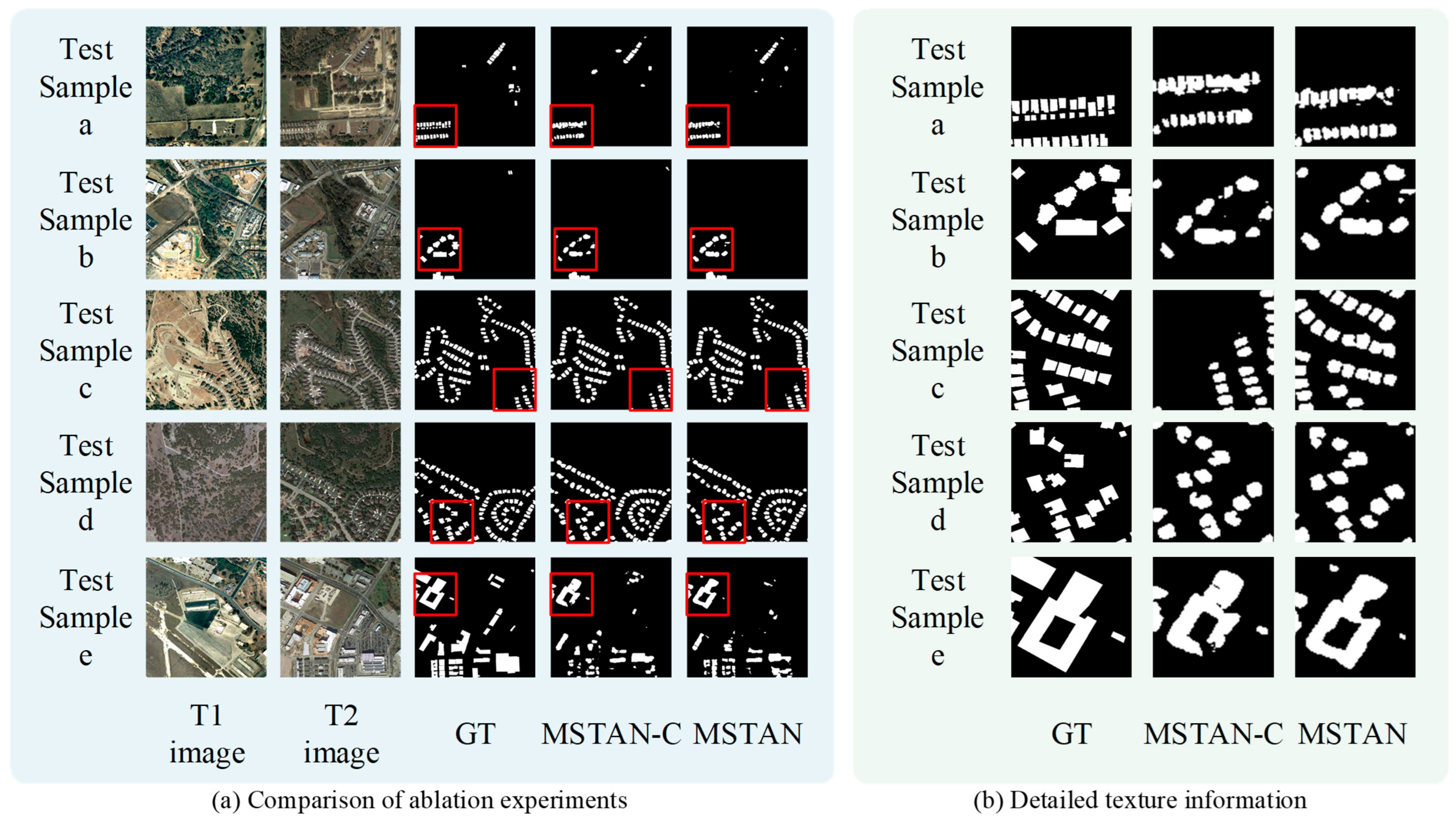
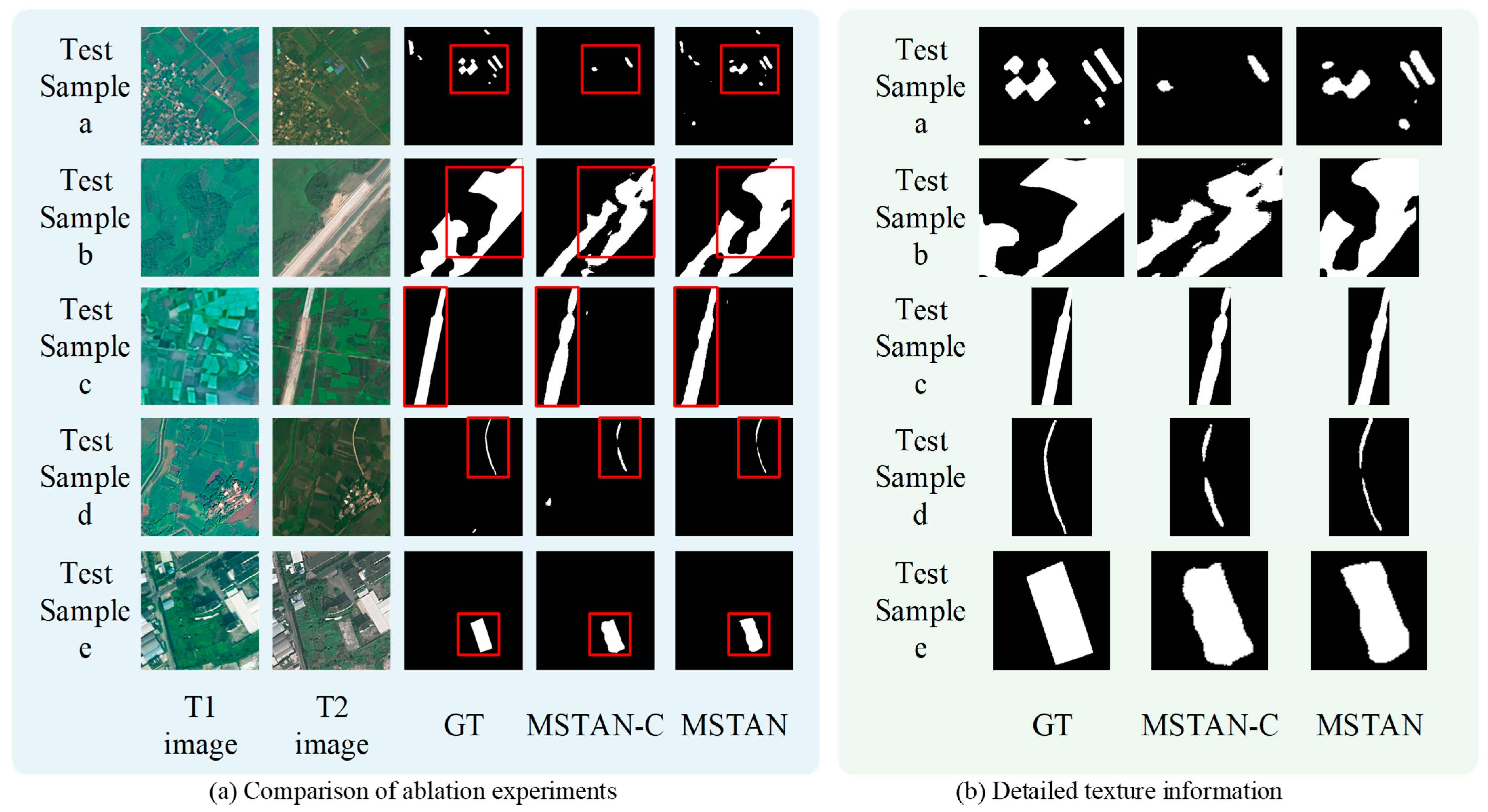
Figure 10 and Figure 11 present the visual comparison of detection results on the two datasets, along with the corresponding detailed information displays.

From the visualization results, MSTAN demonstrates clear advantages on multiple test samples, which is consistent with the aforementioned quantitative analysis findings.

The improvement of MSTAN on the LEVIR-CD dataset is not particularly pronounced. The result generated by MSTAN-C exhibits irregular edges in the red-boxed region (e.g., test sample e), whereas the change region produced by MSTAN shows higher shape fidelity to the ground truth, with smoother and more accurate boundaries. This observation corresponds to the improvements in the IoU and F1-score metrics of MSTAN on the LEVIR-CD dataset in the quantitative analysis, indicating that the four-layer ASFF module enables more precise reconstruction of the morphology of changed regions and enhances the intersection-over-union ratio. The performance improvement of MSTAN is more significant on the CLCD dataset. The region detected by MSTAN-C not only deviates in shape but also contains several missed detections (e.g., test sample a). The detected edges are less smooth and continuous (e.g., test sample a). In contrast, MSTAN’s detection results are closer to the ground truth, with reduced noise. In test sample d, the ground truth contains a thin, elongated change line. MSTAN-C fails to detect this line continuously, exhibiting fragmentation, while MSTAN, although not fully capturing the entire line, handles the edge details more effectively.

However, the four-layer ASFF module clearly has limitations. For instance, noticeable missed detections occur in test sample e on LEVIR-CD and test sample b on CLCD, indicating that MSTAN’s Recall metric still needs improvement—this is particularly critical for sensitive target detection. A possible reason is that the four-layer ASFF module may lack sufficient sensitivity to subtle or fine-grained changes.

In summary, the design of the four-layer ASFF module can effectively address the detection challenges in remote sensing image change detection tasks caused by inconsistent target scales and scene variations. The ASFF module is not merely a technical improvement over concatenation-based fusion; rather, it serves as a fusion framework that enhances generalization capability, providing a more robust fusion strategy for change detection tasks.

3.5. Complexity Analysis

To comprehensively evaluate the impact of the four-layer ASFF module on the computational complexity of the model, we analyze the Floating—point Operations (FLOPs) and model Parameters (Params) of MSTAN (the model with the four-layer ASFF module introduced) and MSTAN-C model (the model that uses the concat operation to fuse multi—scale features instead of the four-layer ASFF module) in

Table 7. Comparison table of computational complexity for the four-layer ASFF module.

Project	MSTAN	MSTAN-C
FLOPs (G)	204.472	202.788
Params (M)	41.437	41.027

.

MSTAN is designed to leverage the four-layer ASFF module for adaptive fusion of multi—scale features, aiming to capture the complementary information across different scales more effectively in remote sensing image change detection. In contrast, MSTAN-C adopts a simpler concat operation, which directly concatenates multi—scale features without adaptive weight learning.

From the perspective of FLOPs, MSTAN has 204.472 G FLOPs, while MSTAN-C has 202.788 G FLOPs. The four-layer ASFF module needs to learn adaptive fusion weights for multi—scale features. This process involves operations such as generating weight coefficients for each spatial position and each scale, which introduces additional computational operations. As a result, MSTAN has a slightly higher number of floating—point operations compared to MSTAN-C that uses the concat operation.

Regarding the model parameters, MSTAN has 41.437 M parameters, and MSTAN-C has 41.027 M parameters. The four-layer ASFF module contains network structures responsible for learning fusion weights. These structures, including lightweight convolutional layers for weight generation, bring in a certain number of parameters, leading to a slightly higher parameter count in MSTAN than in MSTAN-C.

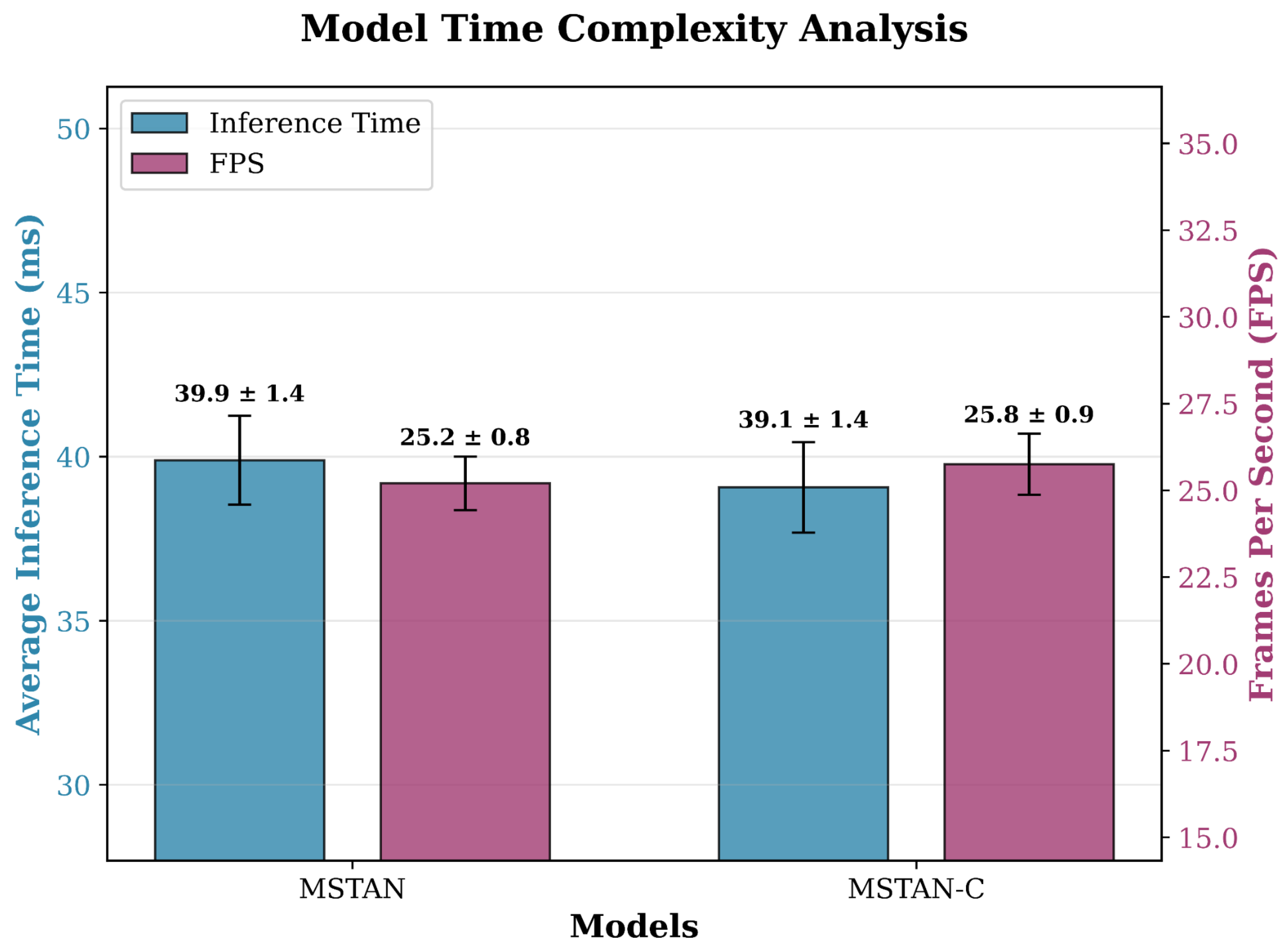
Meanwhile, we conducted five test trials to measure the inference time and FPS (Frames Per Second) metrics on the same input image pair. For each trial, the average inference time and FPS were computed over 100 forward passes with identical input data. The experimental results are presented in

Table 8. Display of the inference time and FPS metrics results.

Number	MSTAN		MSTAN-C
	Inference Time (ms)	FPS	Inference Time (ms)	FPS
1	38.34	26.08	36.77	27.20
2	37.93	26.37	36.78	27.19
3	38.55	25.94	36.21	27.61
4	38.69	25.85	43.57	22.95
5	45.93	21.77	42.01	23.80
Mean	39.89	25.20	39.07	25.75
Std	3.03	1.73	3.09	1.96

. The definition of FPS is given in Equation (9).

$$FPS={\displaystyle \frac{1}{T}}$$

(9)

where T denotes the inference time.

In the table, “Mean” denotes the mean value of repeated trials for each metric, and “Std” represents the standard error of the repeated trials.

Figure 12 shows the error bar plots of inference time and FPS metrics. From these charts, it can be observed that MSTAN has a slightly longer response time and a correspondingly lower FPS compared to MSTAN-C. This is consistent with the earlier analysis of the FLOPs and Parameters metrics. Statistical significance tests across 5 independent training runs confirm the robustness of these results, with standard deviations below 0.3% for all metrics, indicating stable performance free from random training variance.

In summary, the four-layer ASFF module introduces a certain level of computational complexity to the model; however, this increase is attributable to the implementation of more accurate adaptive fusion of multi-scale features. Such adaptive fusion is crucial for enhancing the model’s generalization and robustness. However, for rapid response systems dedicated to specific tasks, the responsiveness of MSTAN remains questionable.

4. Conclusions

This paper proposes MSTAN to address the challenges of multi-scale feature modeling and fusion in remote sensing image change detection. By integrating a multi-scale Transformer encoder and a four-layer ASFF module, MSTAN achieves a balanced enhancement of feature representation and fusion adaptability, which is validated through systematic experiments on the LEVIR-CD and CLCD public datasets.

Extensive comparative experiments on the LEVIR-CD and CLCD datasets demonstrate that MSTAN achieves superior accuracy and robustness, particularly in detecting subtle changes within complex scenes.

Cross-dataset evaluation experiments demonstrate that MSTAN achieves robust generalization capabilities, effectively adapting to data distributions with numerous target categories and multi-scale variations across datasets. It maintains stable and outstanding performance in complex data environments featuring diverse targets.

Ablation experiments further verify that the four-layer ASFF module is the core driver of performance improvement: its adaptive weight learning mechanism enables selective integration of discriminative features across scales, avoiding the static feature aggregation limitations of concatenation.

Despite these promising results, MSTAN has notable limitations. Firstly, MSTAN occasionally underperforms in terms of Recall or Precision when dealing with extremely subtle changes or highly overlapping targets with similar spectral characteristics. This stems from the four-layer ASFF module potentially weakening the correlation between ambiguous regions and reducing the weights of weak signals. Secondly, the four-layer ASFF architecture introduces a certain computational overhead: compared to MSTAN-C, MSTAN increases floating-point operations by 1.684G and model parameters by 0.41M. This may limit its scalability in real-time applications, such as UAV-based disaster monitoring or rapid reconnaissance, where low latency is critical. Thirdly, relying solely on two optical datasets (LEVIR-CD and CLCD) restricts the generalizability of the conclusions. The performance of MSTAN under other data modalities (e.g., SAR (Synthetic Aperture Radar) or hyperspectral imagery) or challenging conditions (e.g., registration errors or illumination variations) remains unverified, representing a key gap for practical deployment.

Future work could focus on addressing these limitations from multiple aspects. Firstly, the four-layer ASFF module could be optimized to better handle ambiguous change scenarios. Secondly, lightweight architectural designs could be explored to improve computational efficiency for real-time applications. Thirdly, evaluation could be extended to more diverse datasets and data modalities. Fourthly, techniques such as domain adaptation and semi-supervised learning could be investigated to enhance the model’s generalization and applicability in scenarios with limited annotation resources.

In summary, MSTAN advances remote sensing change detection by leveraging the synergy of multi-scale Transformer encoding and adaptive feature fusion. Its performance gains and clear mechanism validate the value of adaptive multi-scale fusion. The model holds potential for both civil (agricultural monitoring, disaster assessment) and military (reconnaissance, infrastructure change detection) applications, provided that computational efficiency and generalization are further enhanced.

References

1. Shen, J.; Huo, C.; Xiang, S. Siamese InternImage for Change Detection. Remote Sens. 2024, 16, 3642. [Google Scholar] [CrossRef]
2. Wei, G.; Shi, B.; Wang, C.; Wang, J.; Zhu, X. CINet: A Constraint- and Interaction-Based Network for Remote Sensing Change Detection. Sensors 2025, 25, 103. [Google Scholar] [CrossRef]
3. Yang, J.; Wan, H.; Shang, Z. Enhanced Hybrid CNN and Transformer Network for Remote Sensing Image Change Detection. Sci. Rep. 2025, 15, 10161. [Google Scholar] [CrossRef]
4. Zhou, W.; Jia, Z.; Yu, Y.; Yang, J.; Kasabov, N. SAR Image Change Detection Based on Equal Weight Image Fusion and Adaptive Threshold in the NSST Domain. Eur. J. Remote Sens. 2018, 51, 785–794. [Google Scholar]
5. He, P.; Shi, W.; Zhang, H.; Hao, M. A Novel Dynamic Threshold Method for Unsupervised Change Detection from Remotely Sensed Images. Remote Sens. Lett. 2014, 5, 396–403. [Google Scholar] [CrossRef]
6. Zhou, Z.; Siddiquee, M.M.R.; Tajbakhsh, N.; Liang, J. UNet++: A Nested U-Net Architecture for Medical Image Segmentation. In Proceedings of the International Workshop on Deep Learning in Medical Image Analysis, Granada, Spain, 20 September 2018. [Google Scholar]
7. Caye Daudt, R.; Le Saux, B.; Boulch, A. Fully Convolutional Siamese Networks for Change Detection. In Proceedings of the 2018 25th IEEE International Conference on Image Processing (ICIP), Athens, Greece, 7–10 October 2018; pp. 4063–4067. [Google Scholar]
8. Bandara, W.G.C.; Patel, V.M. A Transformer-Based Siamese Network for Change Detection. In Proceedings of the IGARSS 2022–2022 IEEE International Geoscience and Remote Sensing Symposium, Kuala Lumpur, Malaysia, 17–22 July 2022; pp. 207–210. [Google Scholar]
9. Liu, Z.; Lin, Y.; Cao, Y.; Hu, H.; Wei, Y.; Zhang, Z.; Lin, S.; Guo, B. Swin Transformer: Hierarchical Vision Transformer Using Shifted Windows. In Proceedings of the IEEE/CVF International Conference on Computer Vision, Montreal, BC, Canada, 11–17 October 2021; pp. 9992–10002. [Google Scholar]
10. Liu, X.; Liu, Y.; Jiao, L.; Li, L.; Liu, F.; Zhang, D. Swin Resnetswin Transformers for Change Detection in Remote Sensing Images. In Proceedings of the IGARSS 2023-2023 IEEE International Geoscience and Remote Sensing Symposium, Pasadena, CA, USA, 16–21 July 2023. [Google Scholar]
11. Liu, Z.; Mao, H.; Wu, C.-Y.; Feichtenhofer, C.; Darrell, T.; Xie, S. A ConvNet for the 2020s. In Proceedings of the 2022 IEEE/CVF Conference on Computer Vision and Pattern Recognition (CVPR), New Orleans, LA, USA, 18–24 June 2022; pp. 11966–11976. [Google Scholar]
12. Dosovitskiy, A.; Beyer, L.; Kolesnikov, A.; Weissenborn, D.; Zhai, X.; Unterthiner, T.; Dehghani, M.; Minderer, M.; Heigold, G.; Gelly, S.; et al. An Image Is Worth 16x16 Words: Transformers for Image Recognition at Scale. arXiv 2020, arXiv:2010.11929. [Google Scholar] [CrossRef]
13. Adil, E.; Yang, X.; Huang, P.; Liu, X.; Tan, W.; Yang, J. Cascaded U-Net with Training Wheel Attention Module for Change Detection in Satellite Images. Remote Sens. 2022, 14, 6361. [Google Scholar] [CrossRef]
14. Huo, Y.; Gang, S.; Guan, C. FCIHMRT: Feature Cross-Layer Interaction Hybrid Method Based on Res2Net and Transformer for Remote Sensing Scene Classification. Electronics 2023, 12, 4362. [Google Scholar] [CrossRef]
15. Wu, H.; Yuan, M.; Zhan, T. A Hybrid U-Shaped and Transformer Network for Change Detection in High-Resolution Remote Sensing Images. IET Image Proc. 2024, 18, 1373–1384. [Google Scholar] [CrossRef]
16. Ronneberger, O.; Fischer, P.; Brox, T. U-Net: Convolutional Networks for Biomedical Image Segmentation. In Proceedings of the International Conference on Medical Image Computing and Computer-Assisted Intervention, Munich, Germany, 5–9 October 2015. [Google Scholar]
17. Vaswani, A.; Shazeer, N.; Parmar, N.; Uszkoreit, J.; Jones, L.; Gomez, A.N.; Kaiser, L.; Polosukhin, I. Attention Is All You Need. arXiv 2017, arXiv:1706.03762. [Google Scholar]
18. Chen, H.; Shi, Z. A Spatial-Temporal Attention-Based Method and a New Dataset for Remote Sensing Image Change Detection. Remote Sens. 2020, 12, 1662. [Google Scholar] [CrossRef]
19. Liu, M.; Chai, Z.; Deng, H.; Liu, R. A CNN-Transformer Network with Multiscale Context Aggregation for Fine-Grained Cropland Change Detection. IEEE J. Sel. Top. Appl. Earth Obs. Remote Sens. 2022, 15, 4297–4306. [Google Scholar] [CrossRef]
20. Liu, Y.; Pang, C.; Zhan, Z.; Zhang, X.; Yang, X. Building Change Detection for Remote Sensing Images Using a Dual-Task Constrained Deep Siamese Convolutional Network Model. IEEE Geosci. Remote Sens. Lett. 2021, 18, 811–815. [Google Scholar] [CrossRef]
21. Chen, H.; Qi, Z.; Shi, Z. Remote Sensing Image Change Detection with Transformers. IEEE Trans. Geosci. Remote Sens. 2022, 60, 1–14. [Google Scholar] [CrossRef]
22. Chen, H.; Pu, F.; Yang, R.; Tang, R.; Xu, X. RDP-Net: Region Detail Preserving Network for Change Detection. IEEE Trans. Geosci. Remote Sens. 2022, 60, 1–10. [Google Scholar] [CrossRef]
Figure 1. The architecture of the proposed MSTAN model for change detection. It contains two parts: (1) Multi-scale encoder based on transformer, which utilizes multi-layer Transformer blocks to extract global features of multi-scale changes and employs a Difference Module to capture key differential information. (2) Decoder based on multi-scale adaptive fusion, which utilizes the four-layer ASFF module to fuse multi-scale features, followed by upsampling to restore the feature maps to the original image resolution, and finally outputs a binary change map through a classifier.
Electronics 14 04628 g001
Figure 2. The structure diagram of the Four-layer ASFF module, which consists of two parts: (1) Scale Alignment: linear interpolation upsampling is used to unify the resolutions, achieving spatial scale alignment. (2) Adaptive Fusion: learnable weights are introduced for each layer, and a weighted sum is performed along the channel dimension to obtain a single fused feature map.
Electronics 14 04628 g002
Figure 3. Detail display of adaptive fusion process. In the figure, “1 × 1, 16” denotes a convolutional layer with a kernel size of 1 × 1 and an output channel dimension of 16; similarly, “1 × 1, 4” denotes a convolutional layer with a kernel size of 1 × 1 and an output channel dimension of 4. The rescaled features are firstly passed through a 1 × 1 convolutional layer to generate weight scalar mappings. These mappings are then concatenated and projected into a set of 4-channel weight vectors through another 1 × 1 convolutional layer followed by normalization via the softmax function. Finally, the fused feature is obtained by computing a weighted sum of the rescaled features using the learned weights.
Electronics 14 04628 g003
Figure 9. Detail texture display of interesting regions on cross-dataset.
Electronics 14 04628 g009
Figure 10. Change detection results of the ablation experiments on LEVIR-CD. (a) Change detection results of the two comparative models on the test samples of LEVIR-CD, where the regions marked by red rectangles are the areas of interest; (b) Texture details of the areas of interest.
Electronics 14 04628 g010
Figure 11. Change detection results of the ablation experiments on CLCD. (a) Change detection results of the two comparative models on the test samples of CLCD, where the regions marked by red rectangles are the areas of interest; (b) Texture details of the areas of interest.
Electronics 14 04628 g011
Figure 12. Error bar plot for time complexity analysis.
Electronics 14 04628 g012