Article

End-to-End Camera Pose Estimation with Camera Ray Token

1
Graduate School of Automotive Engineering, Seoul National University of Science and Technology, Seoul 01811, Republic of Korea
2
Technology Research Lab, Ways1, Uiwang Si 16006, Gyeonggi-do, Republic of Korea
3
Department of Mechanical and Automotive Engineering, Seoul National University of Science and Technology, Seoul 01811, Republic of Korea
*
Author to whom correspondence should be addressed.
Electronics 2025, 14(23), 4624; https://doi.org/10.3390/electronics14234624
Submission received: 2 October 2025 / Revised: 19 November 2025 / Accepted: 21 November 2025 / Published: 25 November 2025
(This article belongs to the Special Issue Artificial Intelligence, Computer Vision and 3D Display)

Abstract

This paper proposes an end-to-end method for estimating camera poses using ray regression, a diffusion model-based ray inference approach. The conventional ray regression model outputs moments and directions, which are then converted into the final pose through traditional methods; however, this conversion process can introduce errors. In this work, we replace the conversion process with a deep learning network to achieve more stable pose estimation performance. Furthermore, the proposed model incorporates an additional rendering network for image reconstruction, demonstrating not only camera pose estimation but also the scalability to scene reconstruction. Leveraging the learned features, the model enables image rendering from novel viewpoints. Experimental results demonstrate that the proposed end-to-end method outperforms the conventional ray regression approach under the same training conditions, achieving approximately a 16% improvement in camera pose estimation and a nearly 30% gain in translation accuracy.

1. Introduction

As technology advances, the use of robots is becoming increasingly common in tasks that involve risk or require simple repetitive operations. In the near future, it is expected that robots capable of handling more complex tasks will replace a significant portion of human labor [1,2]. To carry out their tasks, robots must perceive and localize their surroundings using sensors within their working environment. Commonly used sensors include cameras, LiDAR, and RADAR. Among these, cameras differ from the others in that they cannot directly capture 3D information, and the quality of information varies significantly depending on lighting conditions. Nevertheless, cameras are relatively inexpensive, provide color information, and can capture more information at once, making them an essential sensor for the widespread adoption of robots. The advantages of camera sensors, such as low cost and rich information content, make them indispensable in modern robotics. Consequently, the use of camera-only robots is expected to increase. Therefore, achieving accurate pose estimation and real-time performance with cameras is critical, and this challenge is becoming easier to overcome with advances in hardware and the emergence of deep learning.
Ray diffusion [3] is a method based on diffusion models, a class of generative models that have recently demonstrated outstanding performance in image and audio synthesis. However, diffusion models are inherently slow due to their reliance on iterative denoising processes to learn data distributions, which makes real-time performance challenging. The authors of ray diffusion also discussed the performance of ray regression, which uses only a single denoising step. They demonstrated that ray regression achieves strong performance and is well-suited for real-time applications. Ray regression outputs rays characterized by their moments and directions—information that precedes the final pose estimation—and employs traditional methods to infer camera poses [3].
In this study, we adopt the ray regression model, replacing the traditional pose estimation step with a deep learning-based approach. The replacement deep learning architecture is designed to mimic the structure of the conventional method. The concept of rays, originating from NeRF [4], refers to virtual lines that pass through a 3D space and convey information about scene color or depth. Building upon this concept, we extend the model by incorporating a rendering network for additional image reconstruction. Our approach demonstrates stable pose estimation performance, strong generalization ability, and the potential for scalability toward image reconstruction. In particular, accurate and stable camera pose estimation is crucial for visual odometry (VO) and Simultaneous Localization and Mapping (SLAM) in the field of autonomous driving, to which our stable method can make a significant contribution.

2. Related Works

Traditional methods for inferring each camera’s pose using multiple images involve extracting features from images, performing matching across individual images, and then verifying the matches geometrically to remove noise, thereby enabling accurate pose estimation. HF-Net [5] utilizes a feature-extraction network to extract image features, which are then globally matched, followed by local refinement, enabling robust pose estimation across large-scale environments. RelPose [6] extracts features using a CNN and combines the features of two images with a probabilistic relative rotation matrix. From this, a three-layer MLP predicts pose values, enabling the probabilistic evaluation of energy-based symmetry and uncertainty, thereby allowing for accurate pose estimation even with a limited number of images. Pose diffusion [7] employs a diffusion model to progressively optimize camera parameters, leveraging epipolar geometry for fine-tuning. This enables the estimation of both intrinsic and extrinsic camera parameters, regardless of the number of images. RelPose++ [8] extends RelPose to handle multiple images simultaneously and introduces a transformer to estimate camera poses jointly. In particular, instead of normalizing relative to the first camera, it uses the optical centers of all cameras as the reference for translation estimation, thereby improving inference stability. GeoNeRF [9] encodes multiple images using FPNs, applies homography transformations to generate tokens, and combines these tokens with those of the target view for information exchange via a transformer. The density is calculated using the target view tokens from the exchanged tokens, and color values are derived from source image tokens. Rendering is performed through volume rendering, as in NeRF, using the computed density and color values. The performance improves with the addition of more source images, and the approach demonstrates the feasibility of a generalized model that does not require environment-specific training. GNT [10] generalizes NeRF by employing two transformers: a view transformer to define space from source views and a ray transformer for rendering. However, during image reconstruction, it searches for features from sources based on epipolar geometry, which results in slower performance.

3. Method

Ray diffusion [3] divides an image into patches, where the center of each patch is represented as a ray. From the generated rays, the camera’s intrinsic and extrinsic matrices are estimated using an optimization method. In this paper, however, we observed an issue where the intrinsic parameters were estimated differently for the same camera, even though they should remain consistent. Since the intrinsic parameters are already known in most SLAM applications, we proceed under the assumption that they are given. Moreover, since ray diffusion is unsuitable for real-time applications, we base our study on ray regression, which was also discussed in the paper on ray diffusion. Ray regression removes the diffusion process from ray diffusion, achieving approximately 83 times faster inference speed while retaining about 94% of its performance, making it more suitable for real-time systems.

3.1. Pose Estimation Network

In the ray regression, the input image is divided into 16 × 16 patches, and the center ray of each patch is represented in the Plücker coordinate system. According to Plücker coordinates [11], a line can be expressed as r = d , m , which is known to represent an infinite line uniquely. For the central ray of an image patch, the moment is computed as m = p × d , where p R 3 denotes the camera center and d R 3 denotes the ray direction. The conventional model calculates the camera center c from the output rays using Equation (1).
c = a r g m i n p R 3 d , m R p × d m 2
The rotation matrix R and the camera intrinsic matrix K are obtained by first computing the optimal homography matrix using the DLT method [12], and then applying QR decomposition, where K corresponds to the upper triangular matrix R , and R corresponds to Q. Using the computed RRR, the translation matrix t is then calculated as t = R T c .
However, a discrepancy arises when examining the actual computation of the camera center. Specifically, while the ground truth is given as m = p × d with p = c , when inferring from the predicted d , m of the trained model and recomputing the camera center c as p = d × m , the resulting p may differ from the original p . Consequently, the calculated camera center c inevitably contains some error compared to the true value.
In conclusion, since R , t , K can be computed from m , d through a minimization process, they can reasonably be replaced by a deep learning approach. To address the error occurring in the translation t computed in the ray regression, we introduce an additional network that directly estimates R and t .
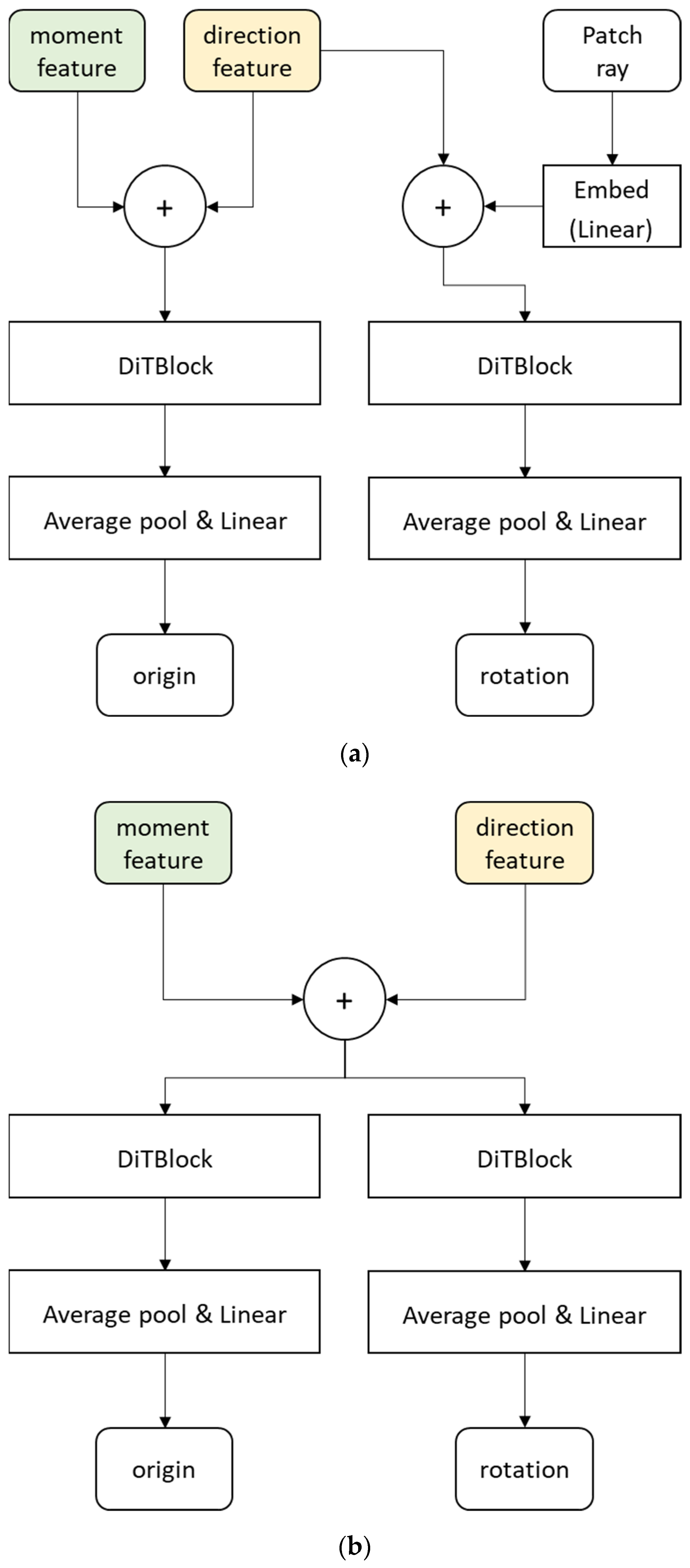
Figure 1 illustrates the original ray regression architecture and the modified design. In the original ray regression, the moment and the direction were simultaneously computed from the Diffusion Transformer (DiT) [13]. However, both the moment and the direction were used for translation estimation when inferring camera pose using traditional methods. In contrast, only the direction was used for rotation estimation, comparing it against the patch-center direction in the NDC coordinate system.
In the modified architecture, the features for computing the moment and direction are separated, allowing each feature to calculate the moment and direction independently. Furthermore, the features extracted before the head are stored and utilized in an additional network designed to estimate the camera pose parameters R , t .
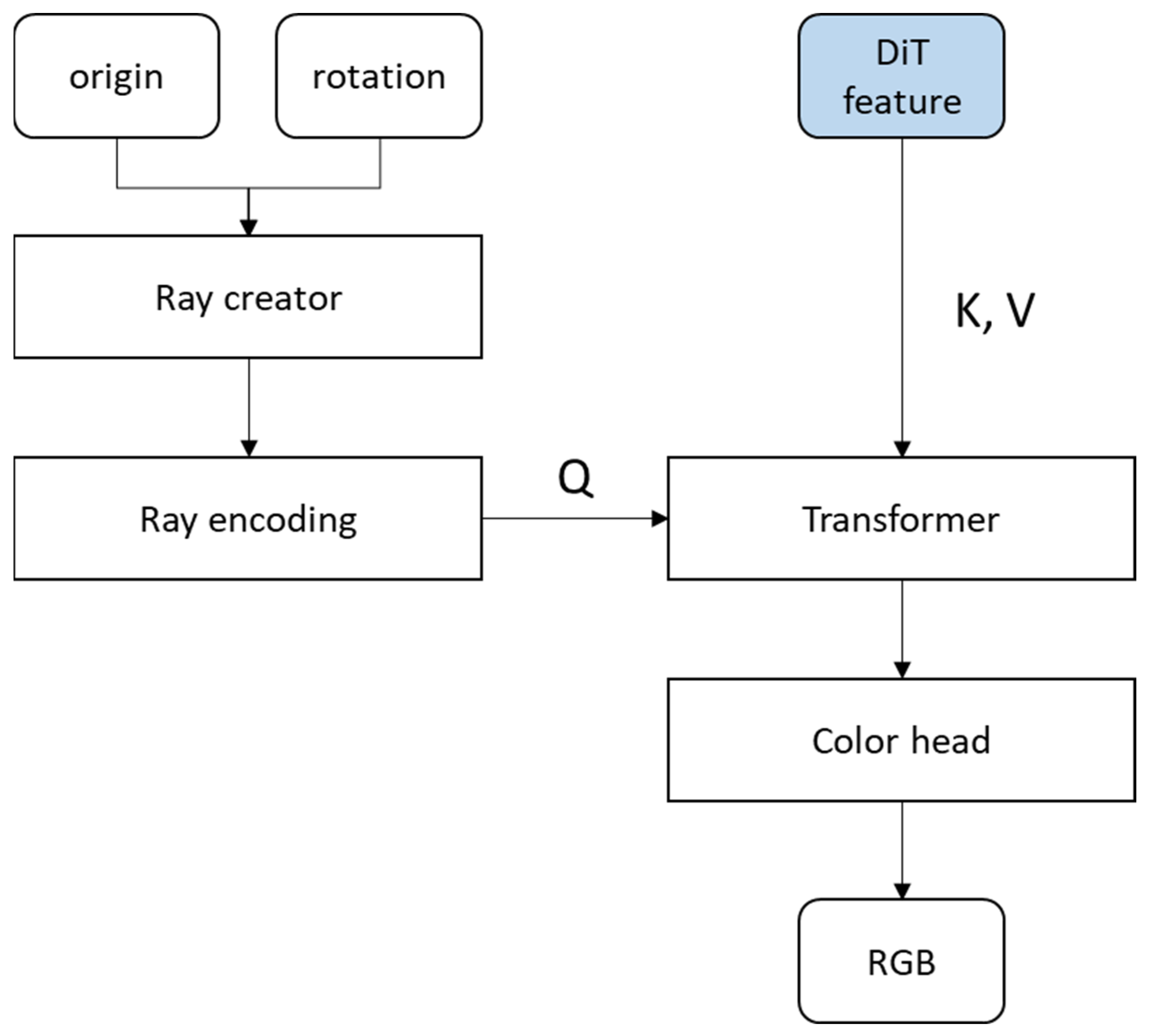
Figure 2 presents the proposed network architecture for estimating R , t . The moment features and direction features used as inputs are taken from the outputs of Figure 1b, with the same color coding. Figure 2a illustrates the architecture constructed using the input format of ray regression: for estimating R , the inferred ray directions and the patch rays are used, while for estimating t , the inferred ray moments and directions are employed. Here, a patch ray refers to the direction vector of a ray expressed in the NDC coordinate system at the center of each patch. Figure 2b, in contrast, shows the architecture that uses only the inferred ray information as input to estimate R , t without providing patch center information.

3.2. Image Rendering Network

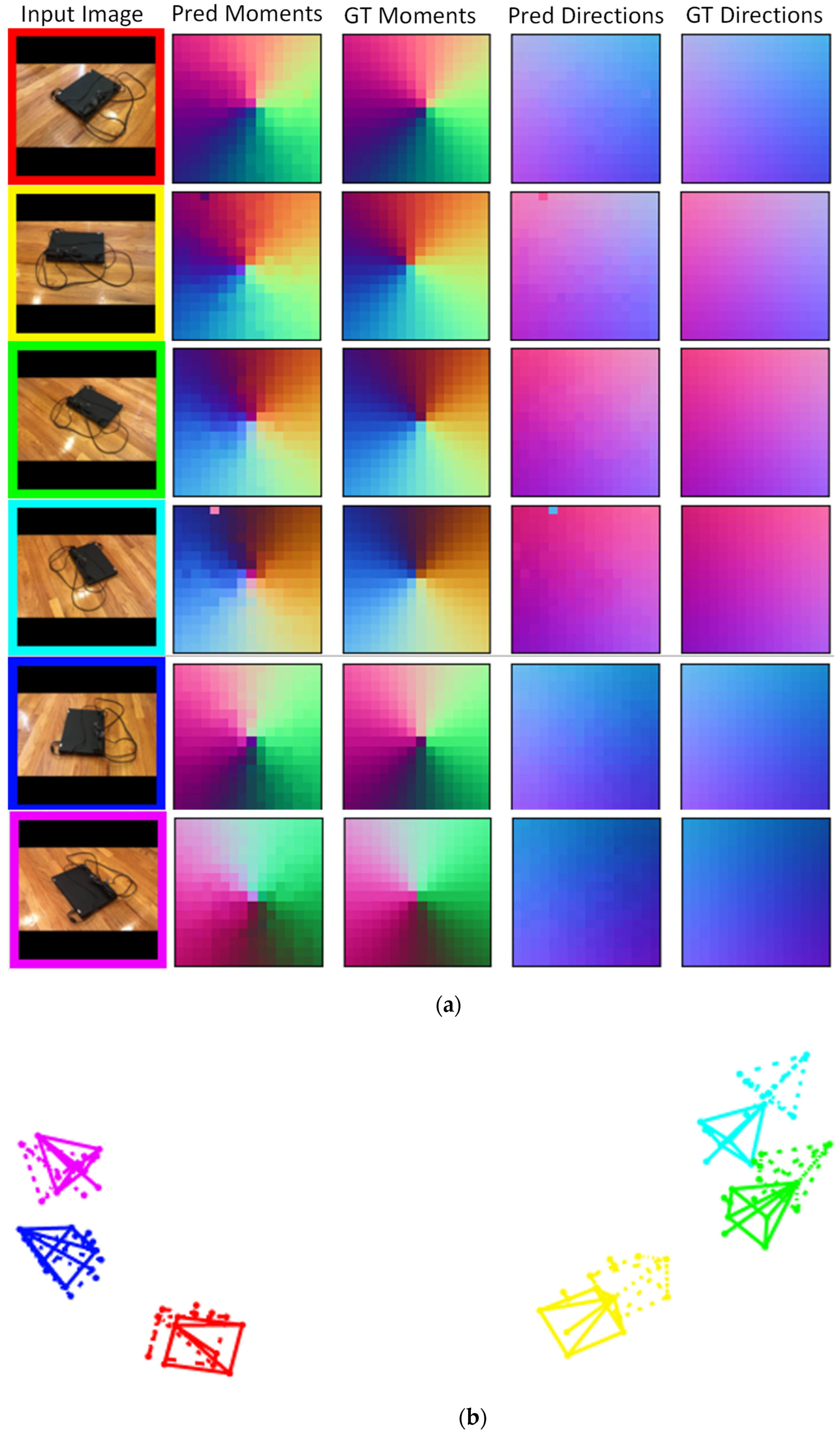
When training the pose estimation network, the feature representation that infers the central ray of each image patch is obtained. This feature can infer the central ray based on the information within the patch and thus can be regarded as a compressed representation of the rays that constitute the patch. By using the compressed image features as keys and values in rendering, and applying the inferred R , t it becomes possible to generate the ray of a specific pixel, which is then used as the query in rendering. In this way, the patch-center ray of a specific ray provides the association needed to retrieve the most relevant feature, allowing the color to be synthesized.
Figure 3 illustrates the architecture of the rendering network. The DiT features are derived from the outputs shown in Figure 1b, which are indicated with the same color coding.

3.3. Loss Terms

Equation (2) represents the loss function used for training. L r a y is a modified version of the loss function employed in ray regression, while L g e o is the loss function used to estimate the camera pose directly.
L = L r a y + L g e o + L r e n d e r
Although ray regression was described as using an L2 loss function defined as the L2 error divided by the number of rays in the set, its actual implementation employed a loss function based on the mean L2 error. In this paper, we revise this by adopting an L2 loss function divided by the total number of rays, as expressed in Equation (3). Here, N r denotes the total number of rays, r ^ i represents the predicted ray vector, and r i denotes the ground-truth ray vector.
L r a y = 1 N r i = 1 N r r ^ i r i 2 2
Equation (4) defines the loss function for camera pose. R ^ denotes the predicted quaternion, R the ground-truth quaternion, t ^ the predicted translation, t the ground-truth translation, and N C the number of cameras. L S represents the Smooth L1 loss.
L g e o = 1 N C i = 1 N C L S R ^ , R L S t ^ , t
Equation (5) defines the loss function for rendering. The loss function commonly used in NeRF-based methods is employed. Here, N R denotes the number of training rays generated using R ,   t . C ^ represents the predicted color, and C is the ground-truth color.
L r e n d e r = 1 N R i = 1 N R C ^ C 2 2

4. Experimental Results

4.1. Datasets and Implementation Details

Based on ray diffusion, we implemented an additional network for estimating camera pose using PyTorch [14]. The training data was taken from CO3Dv2 [15], and training was conducted for 300,000 iterations each on four NVIDIA RTX 3090 GPUs (24GB) and four NVIDIA A5000 GPUs (24GB). CO3D [15] is a video dataset comprising approximately 200 consecutive images of 51 specific object categories, where the ground-truth camera information is provided as estimates obtained using COLMAP. However, this dataset contains some samples with large errors. In the original ray regression, invalid COLMAP estimates were filtered out by discarding data where the ground-truth translation vector exceeded 1 × 10⁵, or the determinant of the rotation matrix was smaller than 0.99 or larger than 1.01. The data sampling method employed the same strategy as the ray diffusion baseline.
In this paper, in addition to those conditions, we further excluded data where (1) the focal length in the NDC coordinate system was larger than 10, which indicates cases where only part of the object was captured, and (2) the size of the principal axis obtained through PCA analysis exceeded 20, to remove biased data. The learning rate was fixed at 1 × 10⁻⁴, the same as in the original, and the batch size was set to 4 per GPU.
Furthermore, in ray regression, the input images were masked to crop only the region containing the object and resized into square images with a 1:1 aspect ratio. In contrast, for potential integration with NeRF in this work, we did not apply masking and instead used the full images, resized to a 1:1 ratio.
The feature extractor used is DINOv2 [16], which is identical to the one employed in ray diffusion. The DiT [13] was also set up with the same architectural specifications as ray diffusion, utilizing 8 layers, 16 multi-heads, and a 1152 hidden layer dimensions.

4.2. Experimental Results and Discussions

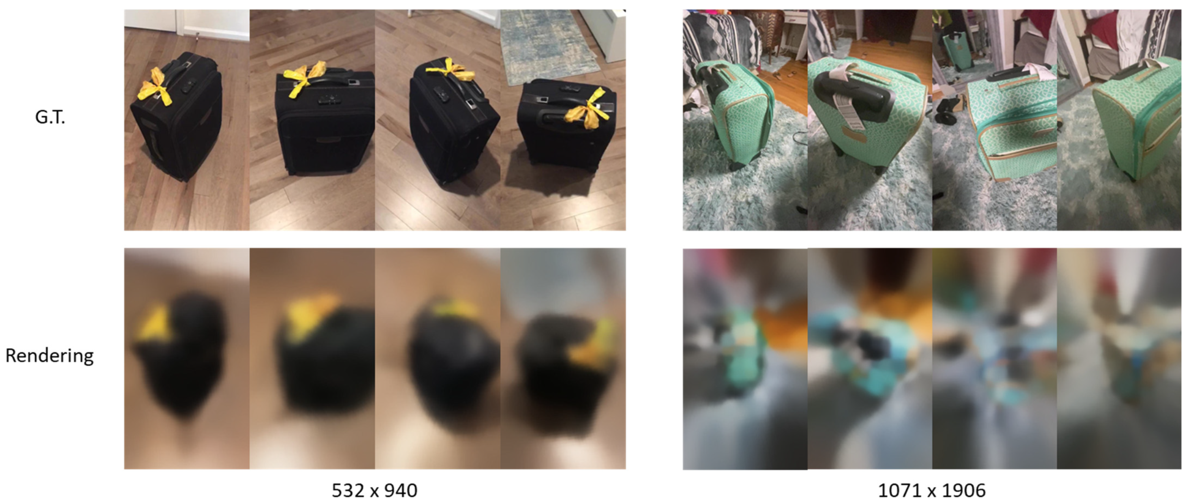
Figure 4 visualizes the input images and the results of the inferred rays. Similar to ray regression, the camera pose estimation network computes the camera pose parameters R , t from the ray moments and directions; therefore, both the moments and directions were trained in the same manner. It can be observed that the predicted ray moments and directions are learned in the same form as the inferred rays produced by ray regression, and that R , t are estimated close to the ground truth. The dotted lines indicate the ground truth, while the solid lines represent the visualized predicted R , t . Since the full images were used without masking and resized to an aspect ratio of 1, black zero-padding can be observed in the inputs. In the second and fourth columns, failures in predicting patch-center rays occur in the padded regions, which are presumed to cause a degradation in rotation estimation performance.
Table 1 presents the performance evaluation of the rotational component using CO3D, and Table 2 presents the evaluation of the translational component. The evaluation follows the same protocol as in the ray regression. Seen categories refer to object classes included in training, while unseen categories denote object classes not used during training. In addition, since the filtering conditions of the CO3D dataset were modified, the pretrained parameters of ray diffusion and ray regression were used for performance evaluation. Ray regression* denotes the evaluation results obtained when ray regression was retrained under the same conditions, including training iterations, batch size, and additional dataset filtering, as our method. The masking strategy was kept identical to that in the ray diffusion paper. Bold values indicate the best performance compared to ray regression, and underlined values indicate the best performance compared to ray diffusion.
The comparison model in this paper uses block1 and applies a tanh activation function at the final stage of rotation estimation. The proposed method demonstrates superior accuracy in camera translation estimation compared to ray regression and ray diffusion, regardless of whether the evaluation is conducted on unseen categories. In particular, as the number of camera images increases from 3 to 8, ray regression exhibits a performance drop of approximately 15% even within the seen categories. In contrast, our method shows only a decrease of about 0.3%, demonstrating more stable performance.
On the other hand, the accuracy of camera rotation estimation is measured to be about 4% lower than that of ray regression on seen categories. However, in unseen categories, it shows comparable performance to ray regression, suggesting that our method offers better generalization. When the rendering network is also included, the translation estimation performance improves slightly, whereas the rotation estimation performance decreases by approximately 5%. This appears to result from the fact that camera rays are represented in the normalized NDC coordinate system, which lacks sufficient information about the kinematic transformation relationships necessary to accurately describe spatial relations across images. Furthermore, compared to ray regression*, the proposed method achieves, on average, about 16% higher performance in rotation estimation and about 30% higher performance in translation estimation, demonstrating superior accuracy and faster convergence than existing approaches.

4.3. Ablation Studies

Table 3 and Table 4 present the results under various training conditions. In Table 4, Model 1 corresponds to the baseline with block1, while Model 2 additionally applies a tanh activation function for rotation estimation. Using the activation function yields an improvement of about 3% for both seen and unseen categories.
Models 3, 4, and 5 in Table 4 replace the image encoder from DINOv2 [16]’s ViT-S/14 distilled model with the ConvNeXt-T, a tiny version of ConvNeXt [17]. Model 3 utilizes an input resolution of 224 × 224 and processes the output of stage 2, resulting in a 14 × 14 feature map that is similar in size to that of DINOv2. Models 4 and 5 instead employ a doubled input resolution of 448 × 448, which allows stage 3 to also output a 14 × 14 feature map. Compared to Model 1, Model 3 exhibits a performance drop of approximately 50%, and Model 4 shows a drop of about 71%. Model 5, which partially fine-tunes parts of the encoder while following the same configuration as Model 4, reduces the performance degradation to about 38% relative to Model 1.
Although ConvNeXt-T has a comparable computational cost and parameter size to DINOv2 ViT-S/14, it outperforms DINOv2 ViT-S/14 on ImageNet-1k but exhibits poor transfer learning performance. These results indicate that CNN-based encoders require partial fine-tuning during transfer learning to achieve competitive results. Moreover, despite using a deeper encoder, Model 4 performs worse than Model 3, indicating that encoders optimized for the classification domain may be unsuitable when transferred to other tasks.
Another possible reason is that DINOv2 was trained using multiple pretraining datasets with masked autoencoding (MAE), making it more generalizable and less domain-specific than encoders tailored strictly for classification. On the other hand, replacing the encoder with ConvNeXt reduces the memory requirement by approximately 4 GB, and even when the input resolution is doubled, the memory usage remains almost unchanged. This suggests an advantage in handling high-resolution images. Furthermore, ConvNeXtV2 has been reported to guarantee improved performance when pretrained with MAE in a CNN-appropriate manner, indicating a promising direction for future improvements.

4.4. Rendering Quality Analysis

Figure 5 presents the results rendered to the original resolution image via the rendering network. This demonstrates the feasibility of scene rendering by incorporating the rendering network, which takes the DiT features and rays generated by the camera pose estimation network as input.
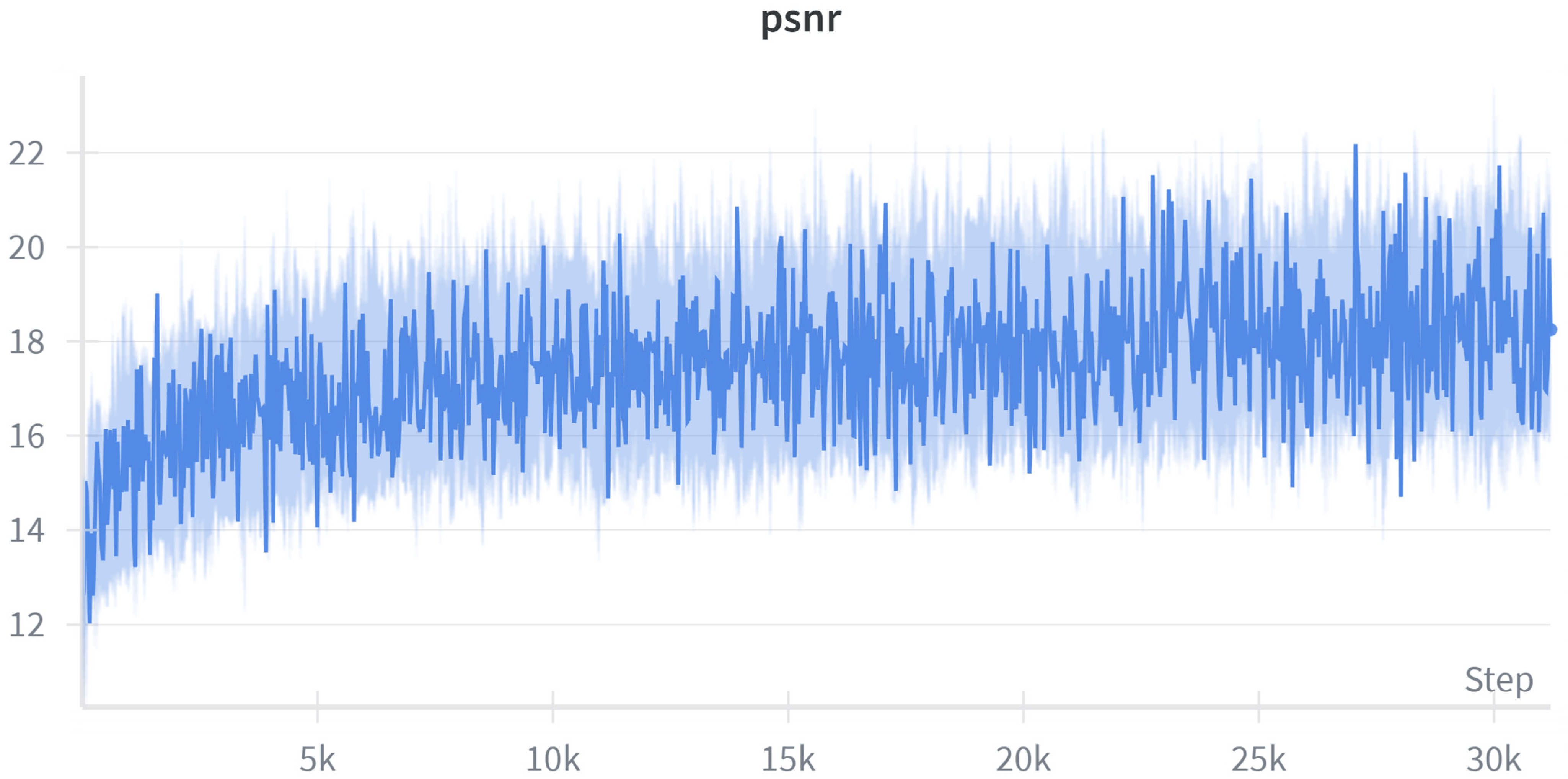
Figure 6 shows the PSNR curve when the model is trained using Block 2 and the rendering loss. It can be observed that the performance improvement becomes significantly slower after approximately 5000 training iterations. This suggests that the current network architecture is insufficient for effectively reconstructing detailed color information.
This limitation in rendering performance is considered to be associated with the lower overall pose estimation performance seen in Table 3 and Table 4 when the rendering loss is applied. Therefore, we anticipate that the scalability aspect can be further complemented by research focused on enhancing the network’s rendering performance.

5. Conclusions

In this paper, we improved the ray regression method—which estimates camera pose by inferring rays from images and computing the pose parameters using traditional methods—by incorporating a deep learning-based network to directly assess the camera pose, thereby enabling more stable inference. Under the same training conditions, the proposed method achieves approximately 16% higher accuracy in rotation estimation and 30% higher in translation estimation, with faster convergence than ray regression. Furthermore, unlike ray regression, which relies on masked images that focus only on regions around the object, our method uses the entire image, resulting in more stable translation estimation performance. However, since the input images are converted to a square aspect ratio (1:1), the added padding regions lack comparable features, which appears to cause a drop of approximately 2% in rotation estimation performance compared to ray regression. We expect that this limitation can be overcome by using unpadded images and incorporating image size information to improve the estimation of patch-center rays, thereby enhancing rotation matrix estimation.
When adding a rendering network to the pipeline, we observed a decrease in rotation estimation performance compared to when the rendering network was not included. This is likely due to discrepancies between the normalized NDC coordinate system, in which the camera pose is computed, and the non-normalized coordinate system in which query rays are represented. This issue could be resolved by requesting queries in the normalized coordinate system or by introducing an additional deep learning module for coordinate transformation for each camera [18,19].
Moreover, as shown by Deformable-DETR [20], comparing only a subset of highly correlated tokens in a transformer decoder yields faster training and inference, as well as higher accuracy, compared to comparing all tokens. Since rays generated from compressed features can appear only in limited views of other cameras, comparing candidate features with higher correlation would be more effective than comparing all image features. Finally, high-resolution images are required to detect small objects such as traffic signs or lights. Since CNN-based features enable scaling to higher resolutions without significantly increasing computational cost, future research should also explore leveraging such features to improve performance. Crucially, the enhanced stability in camera pose inference demonstrated by our End-to-End deep learning network lays a robust foundation for future work, and we intend to proceed with research focused on Simultaneous Localization and Mapping (SLAM).

Author Contributions

Conceptualization, J.-W.K. and J.-E.H.; methodology, J.-W.K. and J.-E.H.; software, J.-W.K.; validation, J.-W.K.; formal analysis, J.-W.K.; investigation, J.-W.K.; resources, J.-W.K.; data curation, J.-W.K.; writing—original draft preparation, J.-W.K.; writing—review and editing, J.-E.H.; visualization, J.-W.K.; supervision, J.-E.H.; project administration, J.-E.H.; funding acquisition, J.-E.H. All authors have read and agreed to the published version of the manuscript.

Funding

This work was supported by the National Research Foundation of Korea (NRF) through the Korean Government (MSIT) under Grant 2023R1A2C1005870.

Data Availability Statement

The authors do not have permission to share data.

Acknowledgments

This paper is based in part on the author’s Ph.D. dissertation [21].

Conflicts of Interest

The authors declare no conflicts of interest.

References

  1. Zhang, Q.-N.; Zhang, F.-F.; Mai, Q. Robot adoption and laber demand: A new interpretation from external completion. Technol. Soc. 2023, 74, 102310. [Google Scholar] [CrossRef]
  2. Kojima, T.; Zhu, Y.; Iwasawa, Y.; Kitamura, T.; Yan, G.; Morikuni, S.; Takanami, R.; Solano, A.; Matsushima, T.; Murakami, A.; et al. A comprehensive survey on physical risk control in the era of foundation model-enabled robotics. arXiv 2025, arXiv:2505.12583v2. [Google Scholar] [CrossRef]
  3. Zhang, J.Y.; Lin, A.; Kumar, M.; Yang, T.-H.; Ramanan, D.; Tulsiani, S. Camera as rays: Pose estimation via ray diffusion. In Proceedings of the International Conference on Learning Representations (ICLR), Vienna, Austria, 7–11 May 2024. [Google Scholar]
  4. Mildenhall, B.; Srinivasan, P.; Tancik, M.; Barron, J.T.; Ramamoorthi, R.; Ng, R. NeRF: Representing scenes as neural radiance fields for view synthesis. In Proceedings of the European Conference on Computer Vision (ECCV), Glasgow, UK, 23–28 August 2020. [Google Scholar]
  5. Sarlin, P.-E.; Cadena, C.; Siegwart, R.; Dymczyk, M. From coarse to fine: Robust hierarchical localization at large scale. In Proceedings of the IEEE/CVF Conference on Computer Vision and Pattern Recognition, Long Beach, CA, USA, 15–20 June 2019; pp. 12716–12725. [Google Scholar]
  6. Zhang, J.Y.; Ramanan, D.; Tulsiani, S. Relpose: Predicting probabilistic relative rotation for single objects in the wild. In Proceedings of the European Conference on Computer Vision, Tel Aviv, Israel, 23–27 October 2022; pp. 592–611. [Google Scholar]
  7. Wang, J.; Rupprecht, C.; Novotny, D. Posediffusion: Solving pose estimation via diffusion-aided bundle adjustment. In Proceedings of the IEEE/CVF International Conference on Computer Vision, Paris, France, 1–6 October 2023; pp. 9773–9783. [Google Scholar]
  8. Lin, A.; Zhang, J.Y.; Ramanan, D.; Tulsiani, S. Relpose++: Recovering 6d poses from sparse-view observations. In Proceedings of the 2024 International Conference on 3D Vision (3DV), Davos, Switzerland, 18–21 March 2024; pp. 106–115. [Google Scholar]
  9. Johari, M.M.; Lepoittevin, Y.; Fleuret, F. Geon erf: Generalizing nerf with geometry priors. In Proceedings of the IEEE/ CVF Conference on Computer Vision and Pattern Recognition, New Orleans, LA, USA, 18–24 June 2022; pp. 18365–18375. [Google Scholar]
  10. Wang, P.; Chen, X.; Chen, T.; Venugopalan, S.; Wang, Z. Is attention all that nerf needs? arXiv 2022, arXiv:2207.13298. [Google Scholar]
  11. Plücker, J. Analytisch-Geometrische Entwicklungen, 2nd ed.; GD Baedeker: Essen, Germany, 1828. [Google Scholar]
  12. Abdel-Aziz, Y.I.; Karara, H.M.; Hauck, M. Direct linear transformation from comparator coordinates into object space coordinates in close-range photogrammetry. Photogramm. Eng. Remote Sens. 2015, 81, 103–107. [Google Scholar] [CrossRef]
  13. Peebles, W.; Xie, S. Scalable diffusion models with transformers. In Proceedings of the IEEE/CVF International Conference on Computer Vision, Paris, France, 1–6 October 2023; pp. 4195–4205. [Google Scholar]
  14. Paszke, A. Pytorch: An imperative style, high-performance deep learning library. arXiv 2019, arXiv:1912.01703. [Google Scholar]
  15. Reizenstein, J.; Shapovalov, R.; Henzler, P.; Sbordone, L.; Labatut, P.; Novotny, D. Common objects in 3d: Large-scale learning and evaluation of real-life 3d category reconstruction. In Proceedings of the IEEE/CVF International Conference on Computer Vision, Montreal, QC, Canada, 10–17 October 2021; pp. 10901–10911. [Google Scholar]
  16. Oquab, M.; Darcet, T.; Moutakanni, T.; Vo, H.; Szafraniec, M.; Khalidov, V.; Fernandez, P.; Haziza, D.; Massa, F.; El-Nouby, A.; et al. Dinov2: Learning robust visual features without supervision. arXiv 2023, arXiv:2304.07193. [Google Scholar]
  17. Liu, Z.; Mao, H.; Wu, C.-Y.; Feichtenhofer, C.; Darrell, T.; Xie, S. A convnet for the 2020s. In Proceedings of the IEEE/CVF Conference on Computer Vision and Pattern Recognition, New Orleans, LA, USA, 18–24 June 2022; pp. 11976–11986. [Google Scholar]
  18. Shi, S.; Wang, X.; Li, H. Pointrcnn: 3d object proposal generation and detection from point cloud. In Proceedings of the IEEE/CVF Conference on Computer Vision and Pattern Recognition, Long Beach, CA, USA, 15–20 June 2019; pp. 770–779. [Google Scholar]
  19. Wang, P.; Liu, Y.; Chen, Z.; Liu, L.; Liu, Z.; Komura, T.; Theobalt, C.; Wang, W. F2-nerf: Fast neural radiance field training with free camera trajectories. In Proceedings of the IEEE/CVF Conference on Computer Vision and Pattern Recognition, Vancouver, BC, Canada, 17–24 June 2023; pp. 4150–4159. [Google Scholar]
  20. Zhu, X.; Su, W.; Lu, L.; Li, B.; Wang, X.; Dai, J. Deformable detr: Deformable transformers for end-to-end object detection. arXiv 2020, arXiv:2010.04159. [Google Scholar]
  21. Kim, J.W. Intergrated Enhancement of SLAM Components Using Deep Learning and Its Applicability. Ph.D. Thesis, Seoul National University of Science & Technology, Seoul, Republic of Korea, August 2025. [Google Scholar]
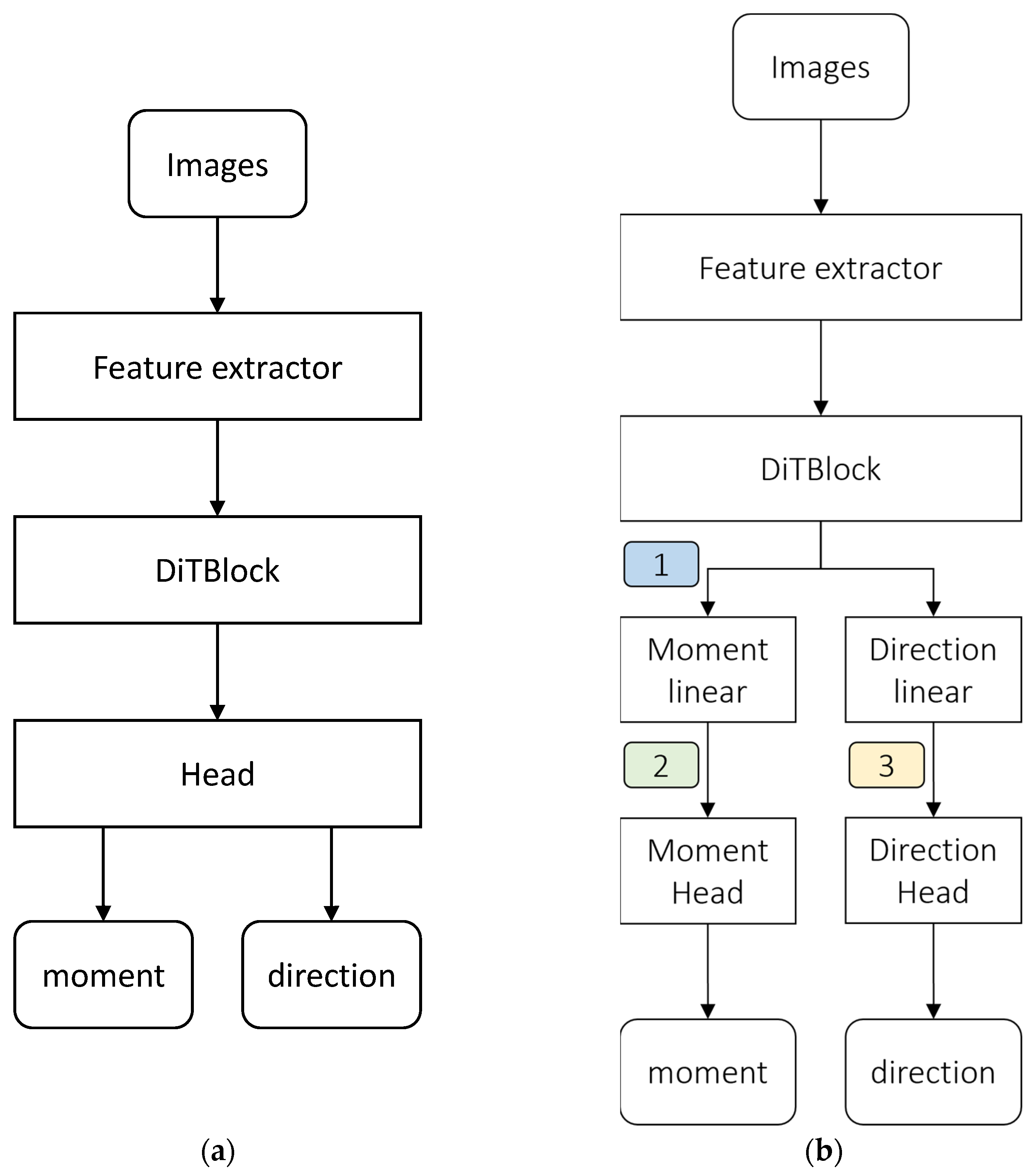
Figure 1. Ray prediction network architectures (a) ray regression prediction architecture (b) our prediction architecture (detailed network structure is represented in Figure 2, and the color of the rectangle is related to Figure 2).
Electronics 14 04624 g001
Figure 2. The proposed network architecture for estimating pose (a) block 1: with patch center information; (b) block 2: without patch center information. The moment feature input is utilized from 2 in Figure 1b, and the direction feature input is utilized from 3 in Figure 1b.
Electronics 14 04624 g002
Figure 3. Rendering network with patch features. The DiT feature used here is illustrated as 1 in Figure 1b.
Electronics 14 04624 g003
Figure 4. Results of the proposed algorithm (a) visualization of ray moments and direction (b) visualization of computed pose (each color corresponds to the color of the input image, where the dashed lines represent the ground truth and the solid lines represent the prediction).
Electronics 14 04624 g004
Figure 5. Results of rendering network.
Electronics 14 04624 g005
Figure 6. PSNR performance curve during training with rendering loss and Block 2.
Electronics 14 04624 g006
Table 1. CO3D camera rotation inference accuracy (@ 15°).
Number of images2345678
Seen Categories
Ray Diffusion [3]92.993.794.094.294.494.594.7
Ray Regression [3]90.290.390.590.991.291.291.1
Ray Regression*79.180.380.480.980.580.580.5
Ours (R + T)87.486.786.586.786.786.786.5
Ours (R + T + Render)80.981.380.880.780.780.780.3
Unseen Categories
Ray Diffusion [3]84.887.388.489.089.089.489.6
Ray Regression [3]81.282.783.484.084.184.484.5
Ray Regression*64.465.164.064.364.264.965.0
Ours (R + T)84.083.383.383.283.183.082.7
Ours (R + T + Render)79.278.278.377.877.577.276.5
Table 2. CO3D camera translation inference accuracy (@ 0.1).
Number of images2345678
Seen Categories
Ray Diffusion [3]10095.091.588.987.586.385.3
Ray Regression [3]10092.386.883.281.079.077.4
Ray Regression*10085.575.469.565.363.260.5
Ours (R + T)10099.799.699.699.599.599.4
Ours (R + T + Render)10099.899.699.699.599.599.4
Unseen Categories
Ray Diffusion [3]10088.583.179.075.774.672.4
Ray Regression [3]10085.576.772.469.166.164.9
Ray Regression*10072.958.551.848.145.143.9
Ours (R + T)10099.398.998.998.598.398.2
Ours (R + T + Render)10099.498.998.898.598.498.3
Table 3. CO3D camera rotation inference accuracy in ablation studies (@ 15°).
Number of images2345678
Seen Categories
1.—Our block1 (R + T)84.583.783.683.783.983.983.9
2.—Rotation w/tanh87.486.786.586.786.786.786.5
3.—ConvNext encoder all freeze *59.558.959.058.959.158.758.6
4.—ConvNext encoder all freeze50.649.549.449.449.649.849.7
5.—ConvNext encoder 0, 1 freeze60.860.360.660.961.060.960.8
6.—Our block1 (R + T + Render)80.981.380.880.780.780.780.3
7.—Our block2 (R + T)87.887.286.986.986.886.786.7
8.—Our block2 (R + T + Render)85.985.385.785.585.685.585.3
Unseen Categories
1.—Our block1 (R + T)82.180.780.480.680.280.380.3
2.—Rotation w/tanh84.083.383.383.283.183.082.7
3.—ConvNext encoder all freeze *45.043.442.042.041.941.340.8
4.—ConvNext encoder all freeze26.024.524.524.424.123.823.5
5.—ConvNext encoder 0, 1 freeze51.251.151.852.352.752.852.9
6.—Our block1 (R + T + Render)79.278.278.377.877.577.276.5
7.—Our block2 (R + T)84.683.382.681.681.881.581.8
8.—Our block2 (R + T + Render)82.381.281.581.081.181.080.6
Table 4. CO3D camera translation inference accuracy in ablation studies (@ 0.1).
Number of images2345678
Seen Categories
1.—Our block1 (R + T)10099.799.699.699.599.599.4
2.—Rotation w/tanh10099.799.699.699.599.599.4
3.—ConvNext encoder all freeze *10099.799.399.198.998.798.6
4.—ConvNext encoder all freeze10099.699.298.998.698.498.2
5.—ConvNext encoder 0, 1 freeze10099.499.098.798.498.398.1
6.—Our block1 (R + T + Render)10099.899.699.699.599.599.4
7.—Our block2 (R + T)10099.899.799.699.499.599.5
8.—Our block2 (R + T + Render)10099.699.298.998.698.498.2
Unseen Categories
1.—Our block1 (R + T)10099.398.998.998.598.398.2
2.—Rotation w/tanh10099.799.699.699.599.599.4
3.—ConvNext encoder all freeze *10098.898.297.697.299.599.4
4.—ConvNext encoder all freeze10098.697.396.795.995.594.9
5.—ConvNext encoder 0, 1 freeze10099.098.197.796.896.896.5
6.—Our block1 (R + T + Render)10099.498.998.898.598.498.3
7.—Our block2 (R + T)10099.198.698.698.598.498.2
8.—Our block2 (R + T + Render)10099.198.999.098.698.598.4
Disclaimer/Publisher’s Note: The statements, opinions and data contained in all publications are solely those of the individual author(s) and contributor(s) and not of MDPI and/or the editor(s). MDPI and/or the editor(s) disclaim responsibility for any injury to people or property resulting from any ideas, methods, instructions or products referred to in the content.