Article

Experimentally-Based Circuit Modeling Validation of a DC-Electrified Railway System for Rail Voltage and Stray-Current Evaluation

1
Department of Industrial and Information Engineering and Economics, University of L’Aquila, 67100 L’Aquila, Italy
2
Department of Industrial Engineering, University of Padua, 35131 Padova, Italy
3
RFI R&D, 00161 Rome, Italy
*
Author to whom correspondence should be addressed.
Electronics 2025, 14(22), 4541; https://doi.org/10.3390/electronics14224541
Submission received: 21 October 2025 / Revised: 10 November 2025 / Accepted: 12 November 2025 / Published: 20 November 2025

Abstract

Despite advancements in mitigating stray current in railway systems, and their impact on nearby installations (i.e., pipelines), challenges remain, necessitating ongoing research and close collaboration between academia and the railway industry. This paper describes the relevant results of a joint industry–academia research project focused on the experimental validation of a reduced complexity circuit model to evaluate the rail potential and the associated stray current directly into the soil. It will be shown that the proposed circuit model is adaptable to various railway lines. Using a lumped parameter approach, the model simplifies spatial discretization without sacrificing accuracy; the relevant resistance and admittance parameters at the sub-stations and along the rail return path are identified, and their impact is studied for the subsequent experimental step. Two real scenarios involve two railway segments in southern and central Italy, which are also different in the geological profile of the terrain. The rail voltage along the two lines is measured and compared with the profile predicted by the lumped circuit model showing the latter’s accuracy. The circuit, validated by the experimental measurements, provides an indirect evaluation of the magnitude of the stray current flowing into the earth. Initially designed for uniform terrain, it can be expanded to include surrounding infrastructure and unintended stray current paths. This framework offers broad applicability and precision across diverse railway environments where nearby critical installations require the estimation of the stray current for the possible subsequent development of countermeasures for their reduction.

1. Introduction

Railways constitute a vital component of modern transportation systems, facilitating the efficient movement of passengers and goods over extensive rail networks. However, the electrification of railways, aimed at enhancing performance and sustainability, has introduced environmental complexities and critical issues such as the presence of stray current. Stray current refers to the unintended flow of electric current through unwanted paths, often resulting from the interaction between railway infrastructure and the surrounding environment. These currents can lead to various detrimental effects, including corrosion of metallic structures, interference with signaling systems, and can compromise the safety of railway operations. Especially in the case of DC stray railway systems, in areas close to the railway, stray current is expected, and protective measures are applied to all sensitive installations like pipelines [1,2].
At the heart of the stray current phenomenon lies the rail voltage (Vr), which is the primary driving force behind its occurrence. The rail voltage, influenced by factors such as traction power supply, rail geometry, and earth conditions, is pivotal in shaping the magnitude and distribution of stray current along railway networks. Understanding the intricate interplay between these factors is essential for devising effective mitigation measures to minimize the adverse effects of stray current [3,4,5].
Recent research has shed light on various aspects of stray current in railways, encompassing theoretical investigations and empirical studies aimed at elucidating their underlying mechanisms and devising practical solutions.
In ref. [6], Mariscotti et al. review electrical quantities related to stray current, stray current protection, and corrosion phenomena. These quantities are relevant for stray current monitoring systems (SCMS) and serve as system health indicators. The discussion covers typical system operation, stray current protection system (SCPS) criteria, measurement methods, and desirable SCMS capabilities. In the end, ref. [6] proposes methods to verify the accuracy and effectiveness of existing SCMS using simulated current leakage scenarios.
A simulation environment for stray current is essential for understanding its behavior and mitigating its effects at an earlier stage of the design and of the construction of the rails. Replicating real-world conditions, such as rail voltages and environmental factors, allows researchers and engineers to study the phenomenon comprehensively. Additionally, a simulation environment provides a safe and controlled experimentation platform, minimizing infrastructure and personnel risks.
In ref. [7], the presented work delves into the numerical modeling of stray current distribution in electrified railway networks, employing advanced computational techniques to simulate the complex interactions between railway infrastructure and the surrounding environment. Their findings underscore the significance of accurate modeling in predicting stray current behavior and guiding the design of mitigation strategies tailored to specific railway configurations, as in [8,9].
On the other hand, many studies adopt a holistic approach to stray current in railways. By analyzing factors such as rail voltage, rail geometry, and environmental conditions, these studies provide a nuanced understanding of the stray current problem [10,11,12,13]. In ref. [14], it is demonstrated that a lumped parameter (LP) model, which follows a circuit-based approach, though it might seem less sophisticated compared to a distributed parameter (DP) implementation, does not compromise precision. This is because stray current involves low-frequency or DC phenomena and does not require fine mesh representation along the longitudinal axis to consider the propagation, thereby maintaining a convenient spatial step size. In this context, the numerous scientific contributions regarding the stray current within the DC metropolitan railway (metro) prove invaluable, considering the numerous analogies with the railway system [15,16]. In [17], the proposed model presents a uniform approach for evaluating stray current along metro lines, considering various structures based on current DC metro sections. Specifically, the return current structures in different configurations are customized and installed at each location according to the metro structure. Consequently, stray current can be assessed in DC metro systems with varying structures. The model is validated by comparing test data with simulation data obtained electronically and by modeling the Shenzhen metro line.
Despite significant advancements in understanding and mitigating stray current, challenges persist, necessitating continued research efforts and collaborative initiatives among stakeholders in the railway industry: evolving technology and the increasing complexity of railway networks underscore the importance of ongoing research and knowledge exchange to tackle the stray current problem effectively.
From the analysis of the scientific literature, a further problem emerges related to the circuit modeling of the phenomenon of stray current: the topological complexity of the circuits. This complexity, certainly due to the search for greater accuracy in representing the various components of the problem under examination, poses two critical points. The greater the number of components to be simulated, the greater the effort to evaluate their value, even theoretically through formulas or other tools, and the more significant the time to compose the final network, with the added possibility of material and/or clerical errors. These problems do not seem compatible with the workflow and timing typical of an industrial environment, such as that of railway infrastructure operators, for whom these calculation models are intended for design applications or predictive maintenance.
This work arises from a research project involving the Italian railway infrastructure operator (RFI) and focuses on the experimental validation, on in-service railway lines, of a reduced-complexity circuit model to evaluate the rail voltage and the associated stray current in the soil. The aim is to show whether a simple circuit model, that can be assembled under full control, quickly and without excessive effort by railway infrastructure operator railway personnel, can evaluate values of the rail potential comparable with those accurately measured along a railway track. The proposed model is adaptable to various types of railway lines and, following the present experimental validation, will be the subject of a subsequent phase of the project, in which it will be made more complex, at the operators’ discretion, by considering articulated soil models, including local defects of rail insulation, and evaluating stray current effects on concrete structures, external victim systems such as pipes, and even power system grounding systems and transformers. The goal is to offer a framework that can be customized according to the specific characteristics of different railway sections. The model can also be tailored to reflect the distinct physical features that define each rail segment.
The proposed circuit model employs a lumped parameter approach, which does not compromise accuracy and obviates the need for fine discretization along the longitudinal axis, thus simplifying the spatial circuit representation of the rail and its environment.
The basic general element of the approach is an elementary LP circuit cell of Π topology (Π-LP): the longitudinal (or “horizontal”) element is built by the series of the rail resistance and inductance (the inductance is not used in this specific contribution because it does not consider any transient phenomena that can have a significant role in the generation of the stray current), and the transversal (or “vertical”) element represents the conductance between the rail and the earth. The model can be expanded to include additional longitudinal and transversal circuit elements to account for the impact of surrounding conductive structural infrastructure. Additionally, it can incorporate elements to represent unintended stray current paths caused by structural defects or discontinuities.
The structure of the paper is the following: Section 2 describes the railway circuit modeling, the elementary LP circuit cell of Π-LP, and the physical meaning associated with its circuit elements. The same Section also describes the equivalent circuit models for the relevant parts of the considered railway sections, such as rails, substations, trains, and boundary (or termination) conditions. Section 3 is devoted to applying the proposed modeling strategy to two different railway tracks (one in the south and one in the center of Italy), where measurement of the rail voltage has been performed. The measured results of the rail voltage are compared with those coming from the circuit simulation to compare them with the circuit simulations to validate the accuracy of the proposed reduced complexity circuit model. From the knowledge of the rail voltage, the stray current in the soil is computed. Section 3.1 describes the topology, measurement, and comparison of the results for the Francavilla Fontana–Brindisi railway line in a flat and dry region of the south of Italy. Section 3.2 describes the topology, measurement, and comparison of the results for the Vetralla–San Martino al Cimino railway line in a hilly part of the center of Italy. Section 4 draws some conclusions

2. Railway Circuit Modeling

This section provides a detailed description of the circuit model employed to evaluate the rail voltage and the stray current in a DC railway traction system. This approach facilitates a comprehensive and efficient representation of the electrical properties among the diverse components of the railway system. This will be shown by applying this circuit modeling approach to two case studies presented in the subsequent sections. Specifically, the network employed enables the accurate computation of electric voltages and currents, facilitating the use of analytical methods to solve the set of equations describing the spatial distribution of the electric variables at various points along the railway network [18]. The basic circuit structure used to evaluate rail voltages and their associated stray current in DC railway systems is represented in Figure 1a.
This model includes several key components.
A cascade of elementary Π cells is used to electrically represent the rail and its conductance to ground/earth. Being part of a DC traction system, each cell contains only resistive elements, such as the rail resistance and the rail-to-earth conductance, which will be discussed later. Although the propagation effects are negligible and only two cells (one on the left and one on the right of the train) can be considered, multiple cells are used to create voltage nodes between them, allowing for the computation of rail voltage and current.
In the proposed circuit model, the train is simulated by an equivalent current source (It in Figure 1a) between the overhead contact line and the rail. This current represents the real traction current absorbed by the train and has been recorded on-board of the moving motor coach at each sampled time and position along the track. Given the position of the train the current source in Figure 1a is positioned on the track and its value extracted assigned from the recorded data. The direct availability of the values of the real traction current is not critical for this circuit model, which is oriented to the analysis of the rail voltage and stray currents, and not to other traction issues, neglecting local phenomena involving the interface overhead line and the train.
The traction substations (TPS), modeled by the voltage source ( V s 1 and V s 2 ) and internal resistance ( R s 1 and R s 2 ), provide and regulate the electrical power to the system, ensuring the trains receive consistent electrical current for their operation, [19]. Although the railway system uses a through-feed structure to feed the overhead contact line, that can be modeled as in [19], in the context of the development of a reduced complexity circuit model for the evaluation of the rail voltage, the assumption of a direct connection between the TPS and the contact line is still valid, as also demonstrated in [20,21]. The resistances of the overhead contact line ( R L 1 and R L 2 , based on the longitudinal resistance of the contact line per unit length R L ) between the substation and the train impact the efficiency of power transmission from the traction substation to the trains. The value of RL1 and RL2 depends on the distance of the train (the current source It) from Vs1 and Vs2, respectively. Given the position of the train (position of It), RL1 and RL2 are computed accordingly.
Each Π−LP cell, as shown in Figure 1b is built by the rail resistance ( R r a i l ) which represents the distributed resistance along the train’s path and the conductance between the rail and the earth ( G r e ).
G r e is a particularly sensitive parameter. Several methods exist for measuring rail-to-earth conductance, each with its own advantages and disadvantages. Examples include the Fall-of-Voltage method, the Four-Pole method, Impedance Spectroscopy, and Clamp-on Probes (the latter method measures rail current and voltage without direct electrical contact, allowing for a safer and quicker assessment) [22,23]. In ref. [24], two approaches are proposed to measure the resistance between the rails and the earth, both with and without the need for external supply, discussing their respective advantages and limitations. Choosing the appropriate rail-to-earth conductance measurement method depends on factors such as accuracy requirements, site conditions, and available resources. It is worth mentioning that one of the main practical challenges in measuring rail-to-earth conductance related to an in-service line is the presence of stray current, which is typically three orders of magnitude smaller than the total return current. This significant difference makes it difficult to detect and measure stray current accurately. Measurement uncertainty is heavily impacted by offsets in the total return current, which can obscure the small variations that indicate stray current leakage. Furthermore, environmental factors such as humidity and temperature, soil geology, electromagnetic interference (presence of signaling and automatic traffic control systems), and rail continuity can affect the accuracy and reliability of these measurements. The uncertainty associated with the direct measurement of the rail-to-earth conductance parameter can be effectively managed by developing an accurate and efficient model that utilizes rail voltage measurements available along the railway line. This approach already examined in [24] is not the main focus of this work but will be considered in the future. Moreover, besides the extraction of rail-to-earth conductance proposed, the method in [24] for extracting the stray current is not readily applicable for the reasons and uncertainties discussed above. Therefore, based on the reference rail-to-earth conductance G′re, once the computed rail voltage is verified experimentally, the stray current extracted from the circuit model is considered to be indirectly verified.
The proposed circuit structure enables a swift and straightforward analysis by considering electric currents variations in response to changes in resistance and conductance along the line. In railway systems, the position of trains is constantly changing, influencing the distribution of stray current: lumped parameter models allow for the dynamic simulation of discrete variations without the need to reconstruct the entire model every time the position of a train changes. Furthermore, the Π-LP network can be employed to promptly evaluate the effectiveness of the stray current mitigation system by calculating the ratio between the total stray current and the total rail return current. This, in turn, facilitates the prediction and optimization of mitigation strategies.
Another crucial aspect of the proposed modeling framework is the accurate representation of the grounding of substations in railway systems, which is a critical setup for safety and operational efficiency. In modern DC traction power systems, choosing an appropriate earthing scheme, i.e., by diode/thyristor-earthed or by Rail Potential Control Devices (RPCDs), is an effective way to decrease corrosion intensity and provide safety for personnel [9,25,26].
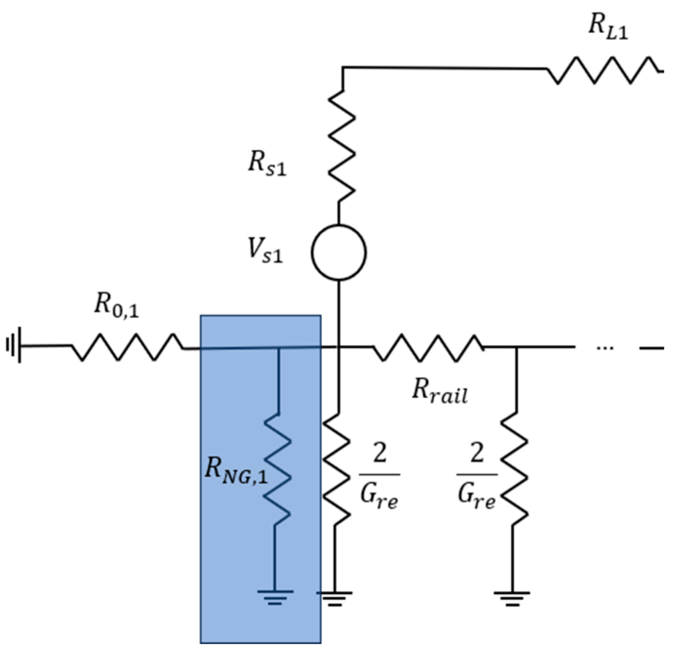
Accurate modeling of substation grounding systems [25] is essential for predicting their performance under various operating conditions and designing effective grounding strategies. Due to the actual characteristics of the substations present in the considered cases, the proposed circuit model represents the substation grounding using an equivalent resistance RNG, as shown in Figure 2 and also proposed in [13].
Measuring the resistance between the negative pole-to-ground in a railway substation can be carried out using various methods such as the Volt-Ampere method (Three-Point Method), the Potential Drop method (Four-Point Method), or the Clamp Meter method [27], each with its own set of challenges such as physical access, environmental influence, electromagnetic interference, or limited accuracy. In this context, a model can be highly useful for indirectly evaluating this resistance value [28]. By leveraging data from accessible electrical measurements, such as voltage and current readings at different points in the system, a well-calibrated model can infer the neutral-to-ground resistance with greater reliability. Moreover, applying a model allows for continuous monitoring and analysis, facilitating the detection of anomalies and trends that might be missed with sporadic direct measurements. This approach not only improves the accuracy of the resistance estimation but also provides significant practical benefits by reducing the need for intrusive testing and enabling more efficient maintenance and troubleshooting processes. In the cases studied in the next paragraphs, the value of R N G has been measured and given by RFI.
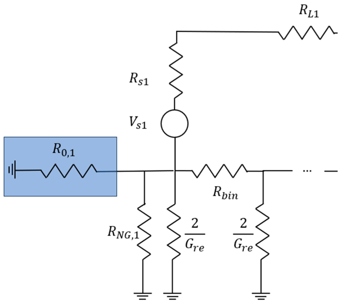
Finally, to account for the running rails upstream and downstream of the railway segment under study, two resistances based on the propagation constant γ of the segment, as in (1), are introduced (2) as proposed in [27].
γ = R r a i l G r e
R 0 = R r a i l G r e
where R r a i l represents the per unit length rail resistance, and G r e denotes the ground conductance per unit length. The locations of these termination resistors in the schematic are highlighted in Figure 3.
This approach balances computational efficiency with enhanced accuracy, allowing for a more realistic representation of the grounding system performance of the substation and the railway sections adjacent to the one under consideration. It also facilitates the seamless implementation of commercial tools for electrical circuits, such as the case studies proposed in Section 3.

3. Experimental Validation

The previous circuit modeling strategy has been applied to two different railway tracks in the south and in the center of Italy. Each track has been modeled according to the proposed technique in Section 2, and the results in terms of rail voltage are compared with the values measured along the two rails. From the spatial distribution of the rail voltage, the circuit model evaluates the associated spatial distribution of the stray current. In Section 3.1, the topology of the Francavilla Fontana–Brindisi railway is described. The same subsection illustrates the relevant concepts and parts of the measurement system used to measure the rail voltage. From the discussion of the comparison between the measured and simulated results, some improvements to the circuit model can also be obtained. Section 3.2 is devoted to the railway from Vetralla to San Martino al Cimino. Because the implemented measurement system is the same as that described in Section 3.1, its description is not repeated in detail. Also, the comparisons between measured and simulated results for this railway are discussed.

3.1. Assessment of Rail Voltage and Stray Current in the Francavilla Fontana–Brindisi Railway Section

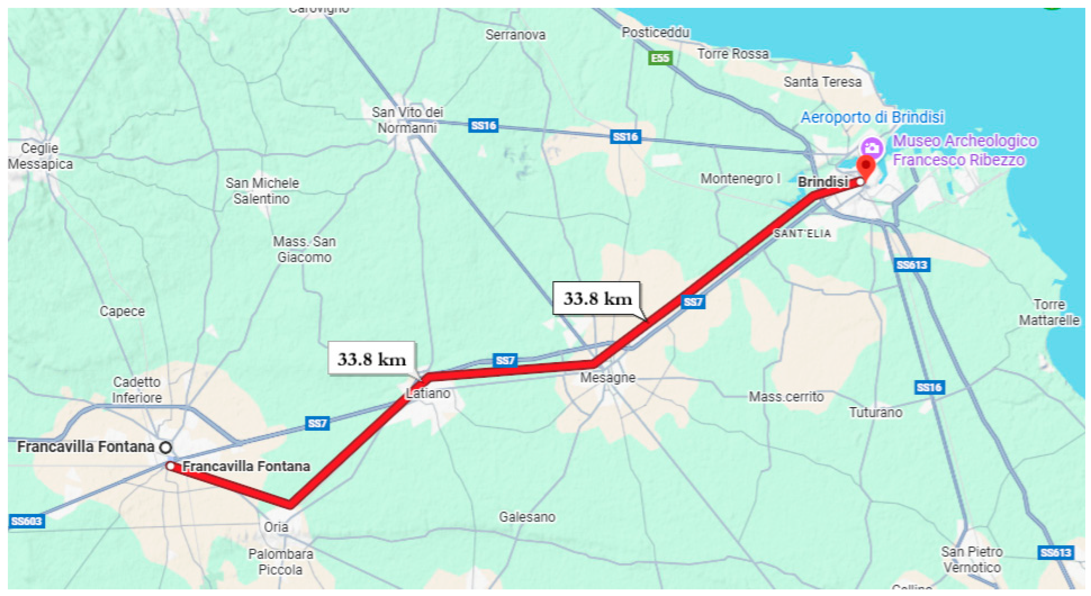
This section focuses on monitoring electrical parameters in the Francavilla Fontana–Brindisi railway line. This activity was prompted by reports of interference from stray current affecting an adjacent gas pipeline. The objective was to experimentally characterize the rail voltage of the traction system under normal operating conditions and to validate it by comparing the circuit model response with the corresponding measured values. Such validation, and the simplified modeling of the stray current paths based on a measured conductance value for the specific railway section under study, allowed the extraction of the order of magnitude of the stray current. Such current magnitude is representative of the specific rail track, and it is readily usable as a first approximation for the design of adjacent pipelines and grounding circuits of nearby industries and power systems. Figure 4 shows the geographical position of the discussed railway.
The developed circuit model (see Section 2), consisting of a cascade of Π-LP cells properly connected to the equivalent circuits of the two power-feeding substations and the current generator of the train (whose magnitude has been taken from the train on-board measurement system), has been solved using the commercial simulator ADS [29], showing the versatility of this software platform. The focus is on simulating single-rail configurations and comparing the simulated data against experimental results to enhance the reliability of predictive maintenance strategies.
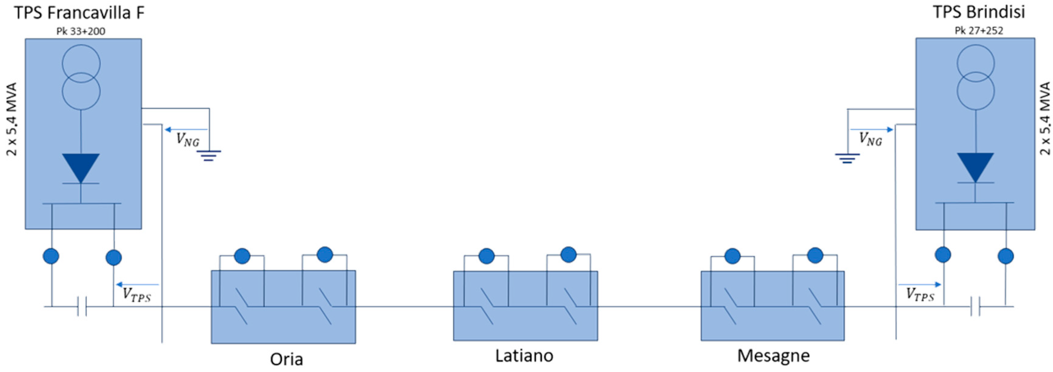
The total railway from Francavilla Fontana to Brindisi is divided into several sections of railway, specifically Francavilla F.–Oria, Oria–Latiano, Latiano–Mesagne, and Mesagne–Brindisi, covering a total length of 33.8 km as reported by the electric traction schematic in Figure 5.
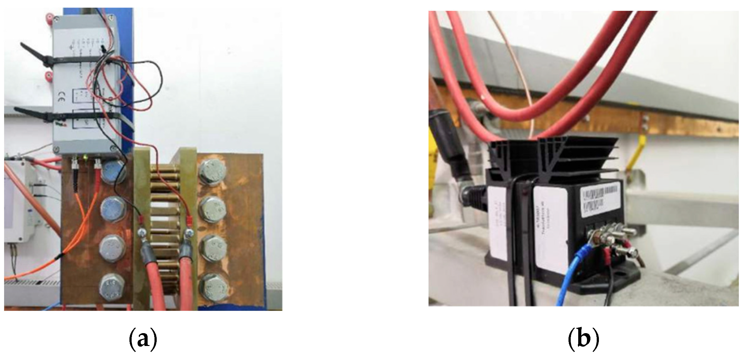
The measurement campaign is based on and developed according to the relevant standards and technical procedures, including [30,31] for electrical safety and measures against stray current and [32] for traction system supply voltages. The monitored section is a single-rail line, powered by the Francavilla Fontana and Brindisi TPSs. The measurements, focused on the spatial distribution of the electrical quantities and not their evolving in time, were conducted within the time frame from 16 February to 18 February. During these two days, several “snapshots” of the line (position of the train, absorbed current, rail voltages) at different instants were taken. At each single “snapshot” the measured data at a single instant, with all measurement devices along the line appropriately synchronized, were detected and recorded to have the spatial distribution of the rail voltage. Different “snapshots” belong to different train positions while the train is moving along the rail track. The data presented in this paper refer to the final recorded measurements after the setup was fine-tuned and made reliable. The instrumentation used for monitoring includes devices for synchronously measuring current and voltage at the points of interest, both in the TPSs and along the electric traction (TE) return circuit. All the measuring instruments have been synchronized to the internal clock of a reference device. The measurements have been recorded by means of a LabVIEW application, detecting and recording the train position and the DC magnitudes of current absorbed by the train and of the rail voltage. The instruments used for detecting such electrical quantities are a Shunt 8000 A/60 mV (LEM International SA, Route du Nant-d’Avril, 152, 1217 Meyrin, Switzerland) for the absorbed current from the power supply at the sub-station, and a LEM/LV-4000 SP6 and A/D Converter NI 9239 (National Instruments Corporation, Austin, TX, USA) for the power supply voltage and the voltage between the negative terminal of the power supply and the earth reference at both the Francavilla Fontana and Brindisi TPSs. Figure 6 shows some details of the installed instrumentation at the Brindisi TPS.
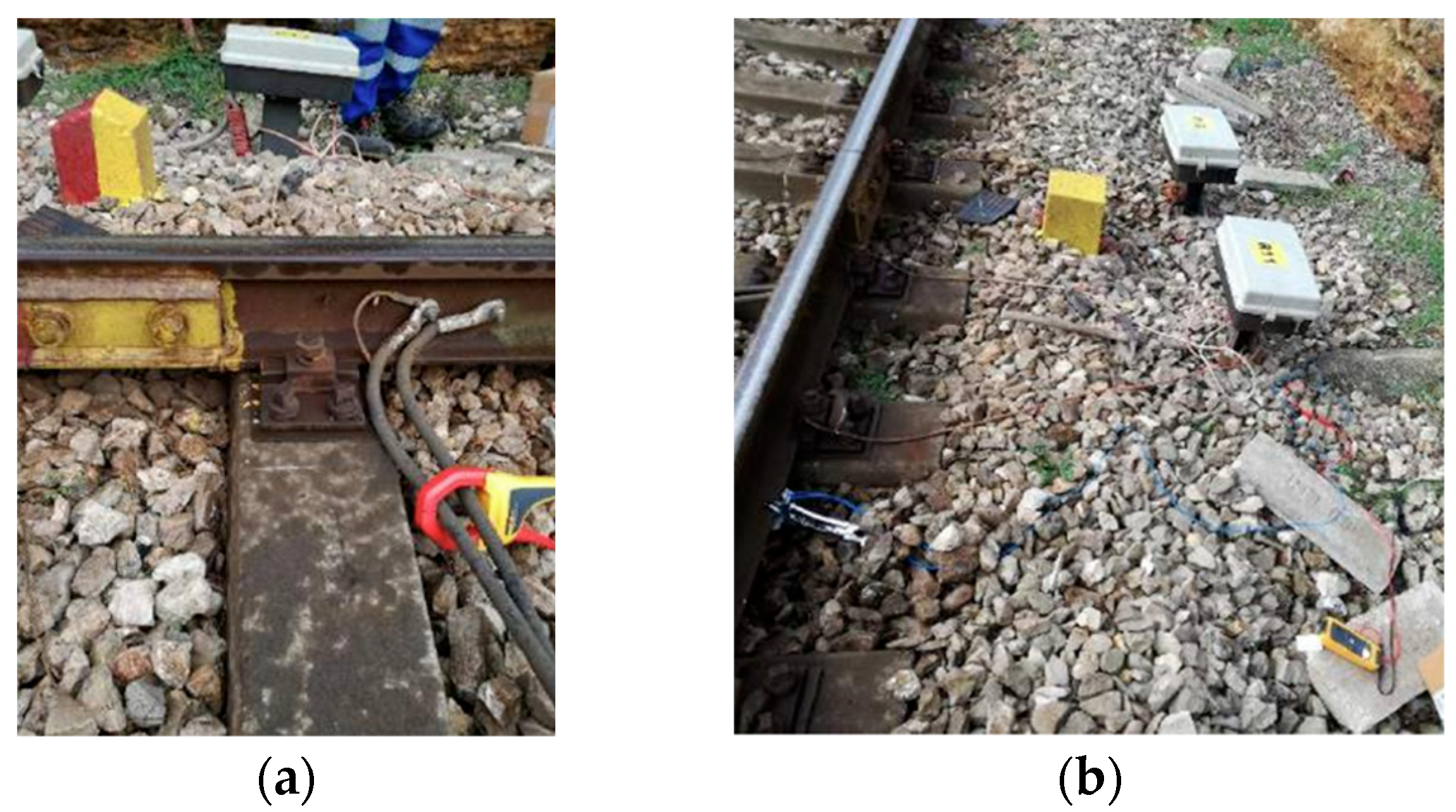
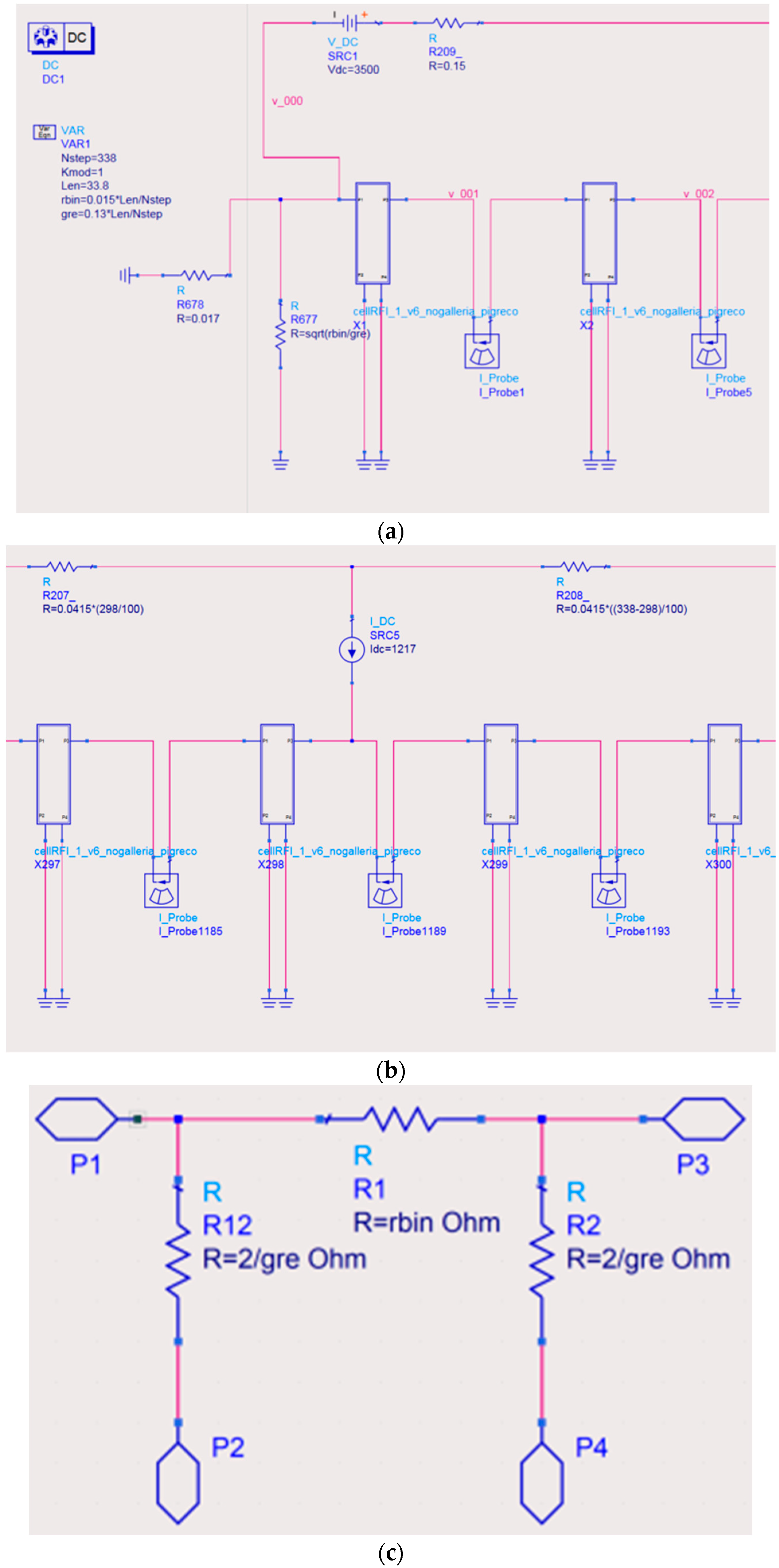
Along the rail section subject under investigation, measurement points were identified where the electrical parameters of the TE return circuit were monitored. These parameters included the current on the return circuit and the rail voltage. The currents were measured on the longitudinal connections of the running rails beyond the extreme points at the following stations: Mesagne (both on the east and west sides), Latiano, Oria, and Francavilla Fontana. Notably, the return currents were measured using amperometric clamps (FLUKE A3003 FC (Fluke Corporation: Everett, WA, USA), range: 0 A to 999.9 A DC/1000 A to 2000 A DC, accuracy: 2% ± 5 digits/2.5% ± 5 digits [33]) installed in the same direction as the return currents toward Brindisi TPS, and the rail voltages were measured using FLUKE V3001 FC (pertinent range: 600 mV to 600 V DC, accuracy: ±0.09% + 3 digits [34]) relative to reference electrodes of the Cu/CuSO4 type as shown in Figure 7. Although the Cu/CuSO4 electrodes are commonly used to measure the impressed voltage on embedded structures, RFI has adopted their use to overcome the difficulties of using rods when the ground has different levels of penetrability or even (although this is not the case in this work) in presence of viaducts or tunnels. Furthermore, the use of electrodes allows operators to select the best spacing between measurement points along the railway line under analysis, offering greater flexibility in their positioning without being tied to the earth and protection circuit. It is also possible to measure the rail potential with respect to the railway earthing rods, which are connected to each TE pole and therefore present along the line every 50/60 m. These electrodes have a voltage reference that remains practically unchanged (except for the possible presence of chlorides in the terrain) in every environment in which they are installed. The circuit is implemented in the ADS and summarized in Figure 8 with an example of termination (Figure 8a), the train source current (Figure 8b), and the elementary Π-LP cell (Figure 8c).
The simulator circuit was configured to reflect the nominal parameters of the railway sections under study, which are reported in Table 1.
The origin of these values comes from nominal technical data and previous measurement campaigns during the regular in-service railway operation. Moreover, the value of G′re was measured only in one position (around the middle of the overall track length and contemporary to the voltage measurement), during the railway operative condition, due to technical and safety constraints imposed by the railway operator. The railway operator employed the procedure defined in [31], specifically Paragraph A.3 of Appendix A, for measuring the rail-to-earth conductance G′re.
The meteorological conditions along the whole railway length during the two-day measurement period were recorded and analyzed. No significant global changes were found or expected in the surface or ground characteristics, and therefore in the conductance. These data are not reported for sake of brevity. The preliminary actions and studies conducted prior to the measurement campaign led to the hypothesis of a homogeneous subsurface geological profile along the railway track under study. As a first approximation for the current analysis, a single measured value of G′re was used and attributed to all the elementary cells (each corresponding to an equivalent length of 0.1 km) of the circuits.
The first analysis concerns the evaluation of the spatial distribution of the rail voltage between Francavilla Fontana and Brindisi when the train is located between the train stations of Mesagne and Latiano.
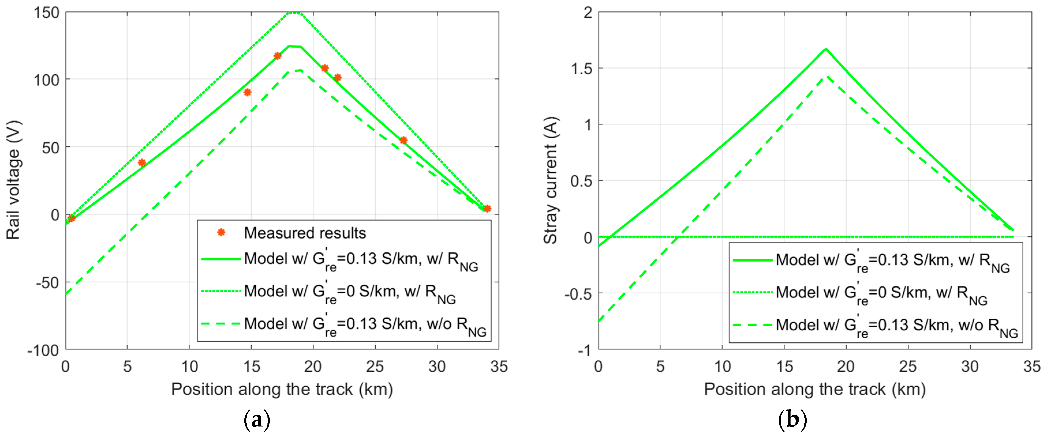
In Figure 9a, the red asterisks (labeled as “Measured results”) show the measured values of the rail voltage at the measurement points. The upper dotted green line (labeled as “Model w/ G r e = 0 S/km, w/RNG”) represents the rail voltage computed in the ideal case with (w/) G r e , the conductance between the rail and earth, whose value is zero, representing full rail-to-earth isolation (the stray current does not flow to the soil). This can be considered a limiting case. The lower dashed green line (labeled as “Model w/ G r e = 0.13 S/km, w/o RNG”) is obtained by simulation when G r e has the value measured along the line and reported in the legend. In this case the model is without (w/o) the presence of RNG at the TPS. A better agreement between measurement and simulated results is obtained along all the rails when the TPS R N G is also introduced with its measured value reported in Table 1. In this case the results are reported by the continuous green line labeled as “Model w/ G r e = 0.13 S/km, w/RNG”.
The stray current, that has not been measured, is only computed by the proposed circuit model starting from the rail voltages, which consider the currents flowing through the vertical G r e branches of the Π−LP cell as
I s t r a y = V r G r e
In Figure 9b the dotted horizontal green line represents the null value of the stray current, evaluated according to (3) when the rails are ideally fully isolated with respect the earth ( G r e = 0 S/km). The slanted dashed and continuous green lines represent the spatial distribution of the stray current when the TPS’s RNG are omitted or considered into the circuit model, respectively.
From now on all the simulation will be performed considering a circuit model with the presence of RNG, for this reason this information will no longer be reported in the legends of the figures.
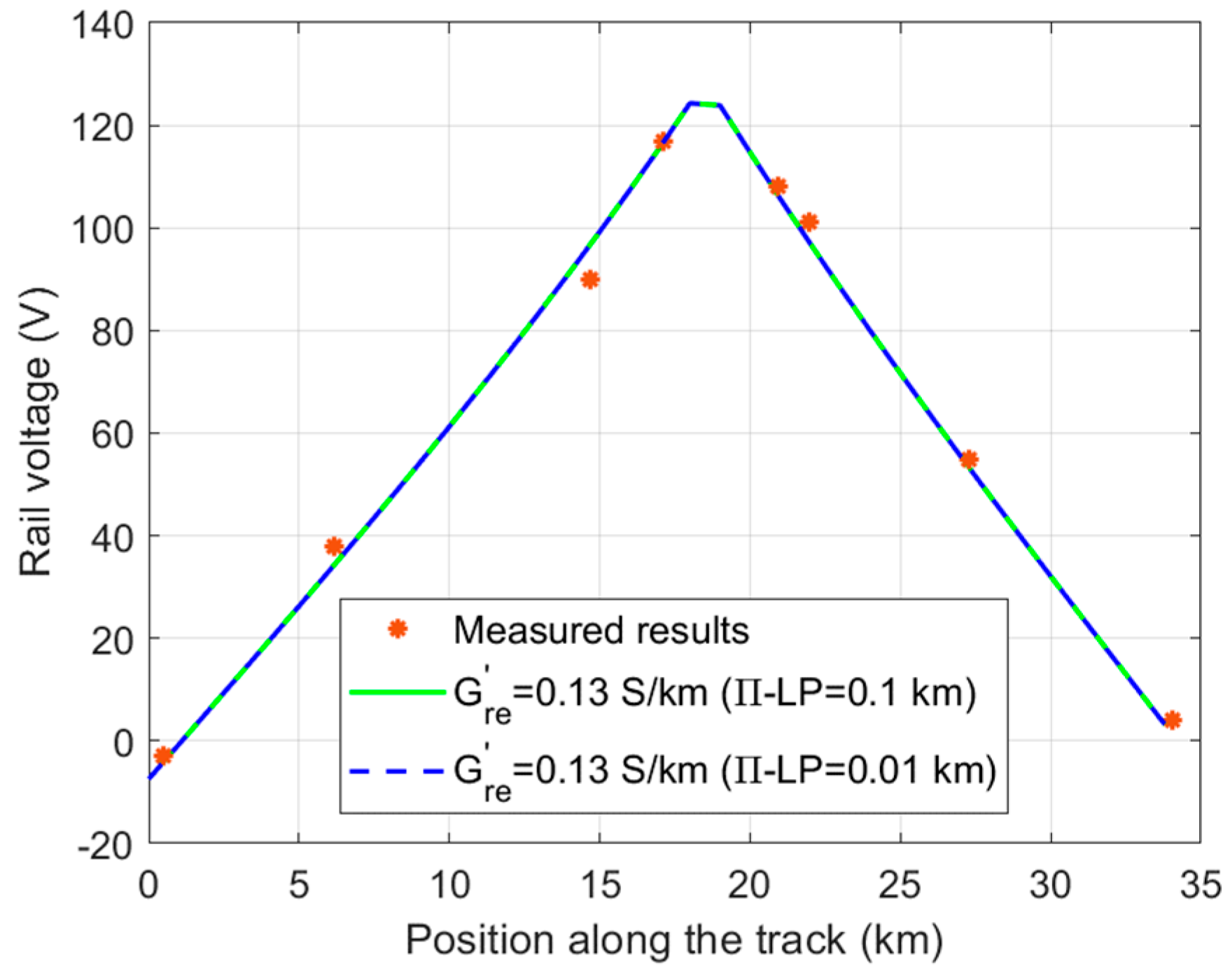
As already mentioned, in the previous simulations the length of each Π-LP cell was 0.1 km. To verify whether the modeling results are dependent on the length of the elementary cell, an additional case is considered with the length of the elementary Π-LP cell of 0.01 km. Figure 10 shows an almost perfect match between the two computed rail voltages based on different length of the elementary cell, thus confirming the validity of the proposed lumped circuit.
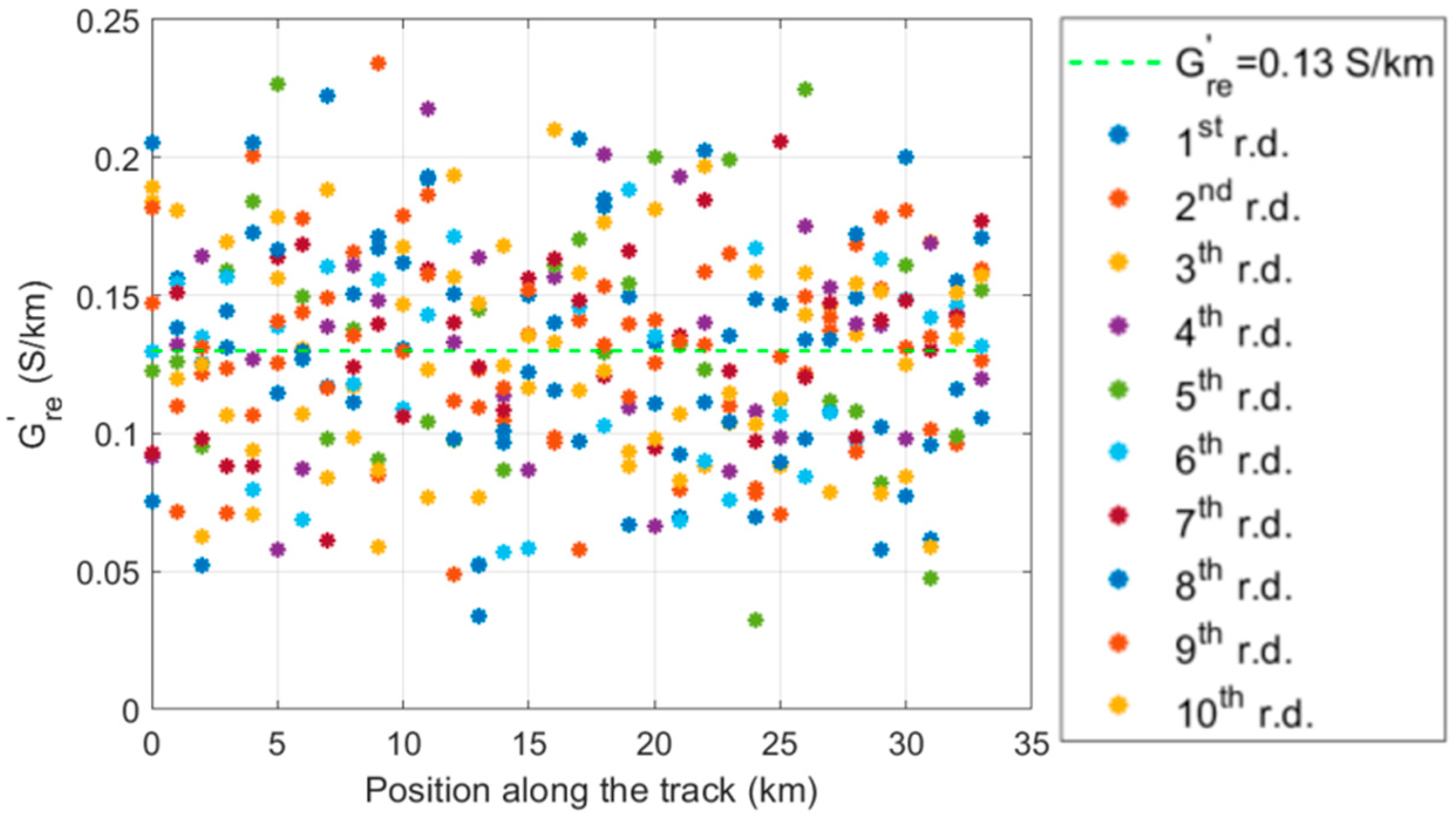
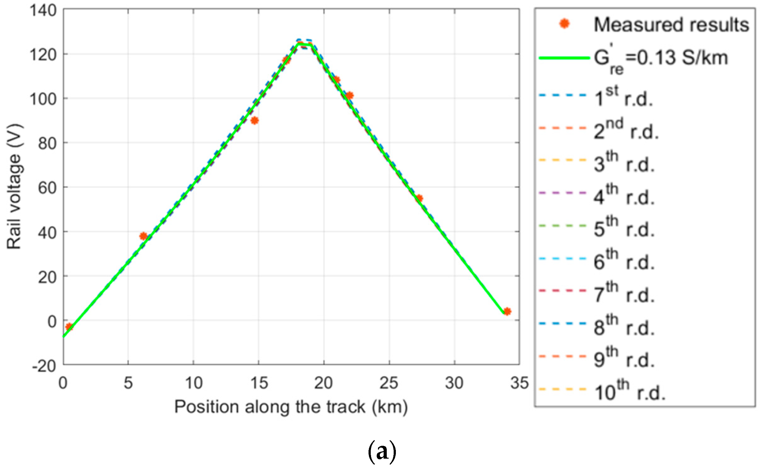
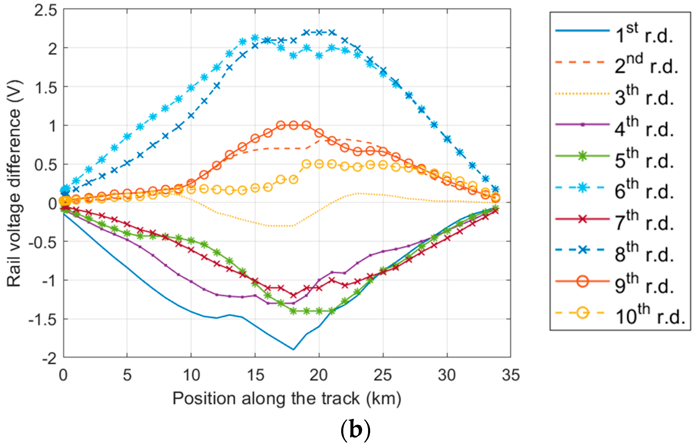
To check the validity and robustness of the assumption of a constant value of G r e along the track, a sensitivity analysis has been carried out. The Francavilla Fontana–Brindisi line is 33.8 km long. Its equivalent circuit is built up by 34 sections, each containing 10 Π-LP elementary cells (the last section has only 8 cells). Each cell has a length of 0.1 km. Ten sets of 34 random values of G r e , one for each kilometer of the line, have been generated. Each set is a random Gaussian distribution (labeled in Figure 11 as “r.d.”) of G r e values with a mean equal to the measured value G r e = 0.13 S/km and a standard deviation σ equal to 30% of the mean value. Considering one set at a time, each value of the generated G r e has been assigned to a section of 10 (or 8 in the case of the last one) Π-LP cells. Figure 11 represents the ten sets of G r e values. Figure 12a compares the measured values of the rail voltage versus the computed values with constant G r e (measured value) and those computed using the ten random distributions of G r e with 30% deviation. The differences in the rail voltage computed with constant G r e and with the ten random Gaussian distributions with 30% deviation are shown in Figure 12b.
As can be observed in Figure 12, the rail voltage differences between the condition of a variable G r e along the line and the case of constant G r e are very small and both conditions are close to the measured (red asterisks) values.
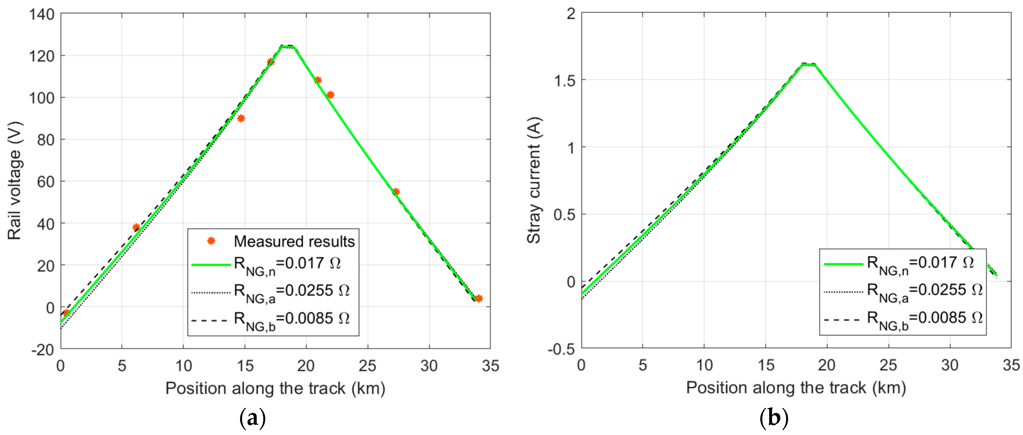
From a quantitative point of view, the maximum difference in rail voltage between constant and variable G r e cases occur at the peaks of the curves with a value of 126.4 V compared to 124.3 V, representing a 1.7% difference. A 30% deviation in G r e leads to rail voltages that are very close (see rail voltage differences in Figure 12b) to each other and to the case where G r e is constant and equal to the measured value, thus aligning closely with the measured values. These results support the validity of the forced assumption (due to the actual lack of other available values) of a constant value of G r e . Although RFI gives R N G in Table 1 as a consolidated value for its TPS, the reduced complexity of the used circuit model allows also a sensitivity analysis of the rail voltage and stray current while varying R N G . Three values of RNG have been considered: the nominal RNG (Table 1) named RNG,n, RNG,a = 1.5·RNG,n = 0.0255 Ω, and RNG,b = 0.5·RNG,n = 0.0085 Ω. Figure 13a reports the measured values of the rail voltage along with the spatial distribution of the rail voltage computed by the circuit model with G’re = 0.13 S/km for all cells and the three different values of RNG. Figure 13b shows the corresponding computed stray current.
One can observe that the value of RNG mainly impacts the magnitude of Vr close to the substations at the ends of the line. This is also confirmed by Table 2 and Table 3 in which the values of Vr and Istray at the ends of the line are reported for the different values of RNG considered in Figure 13.
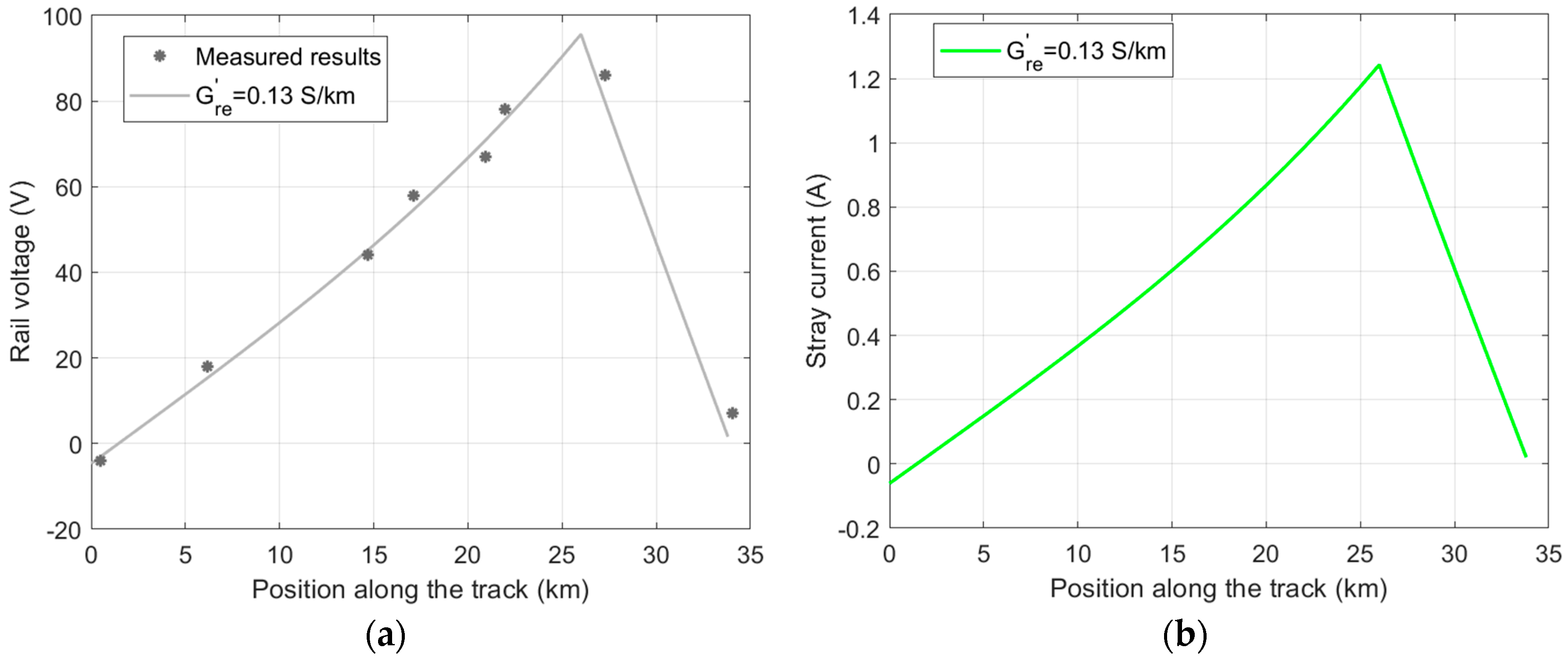
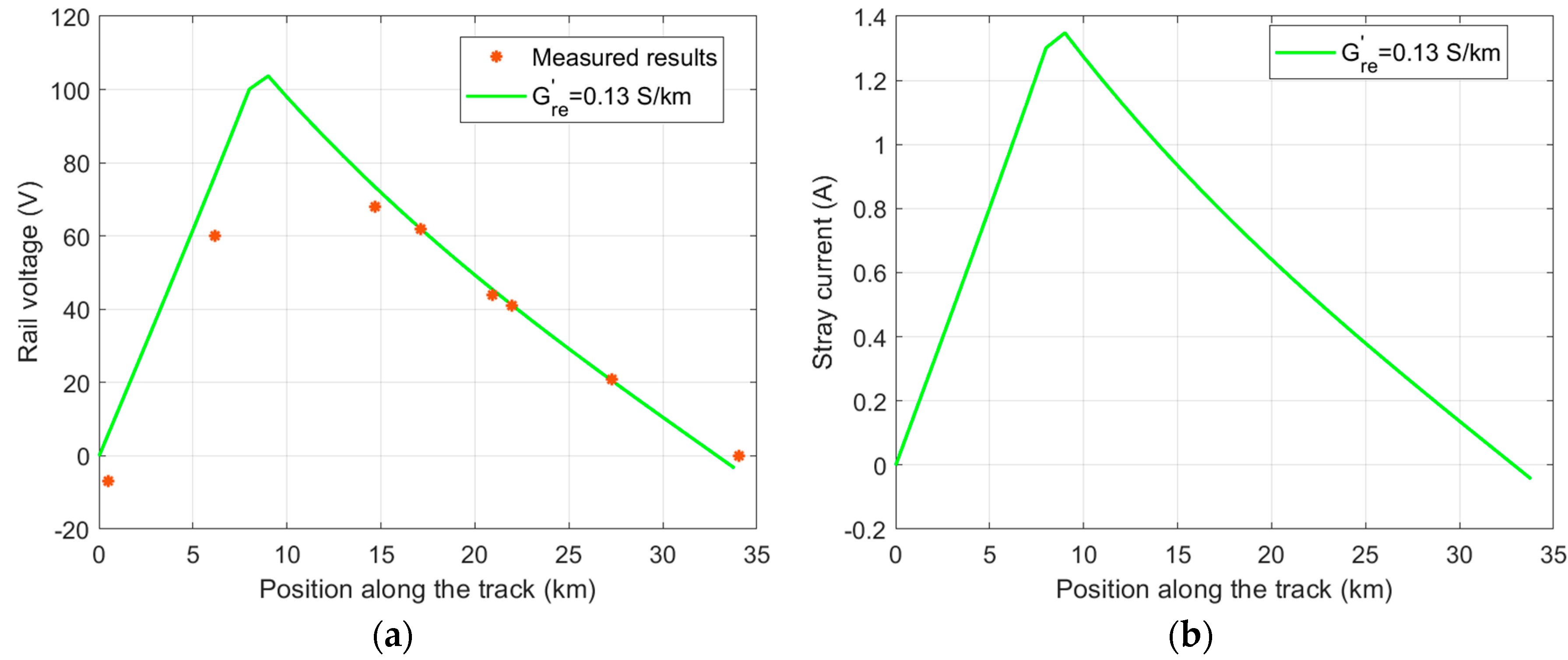
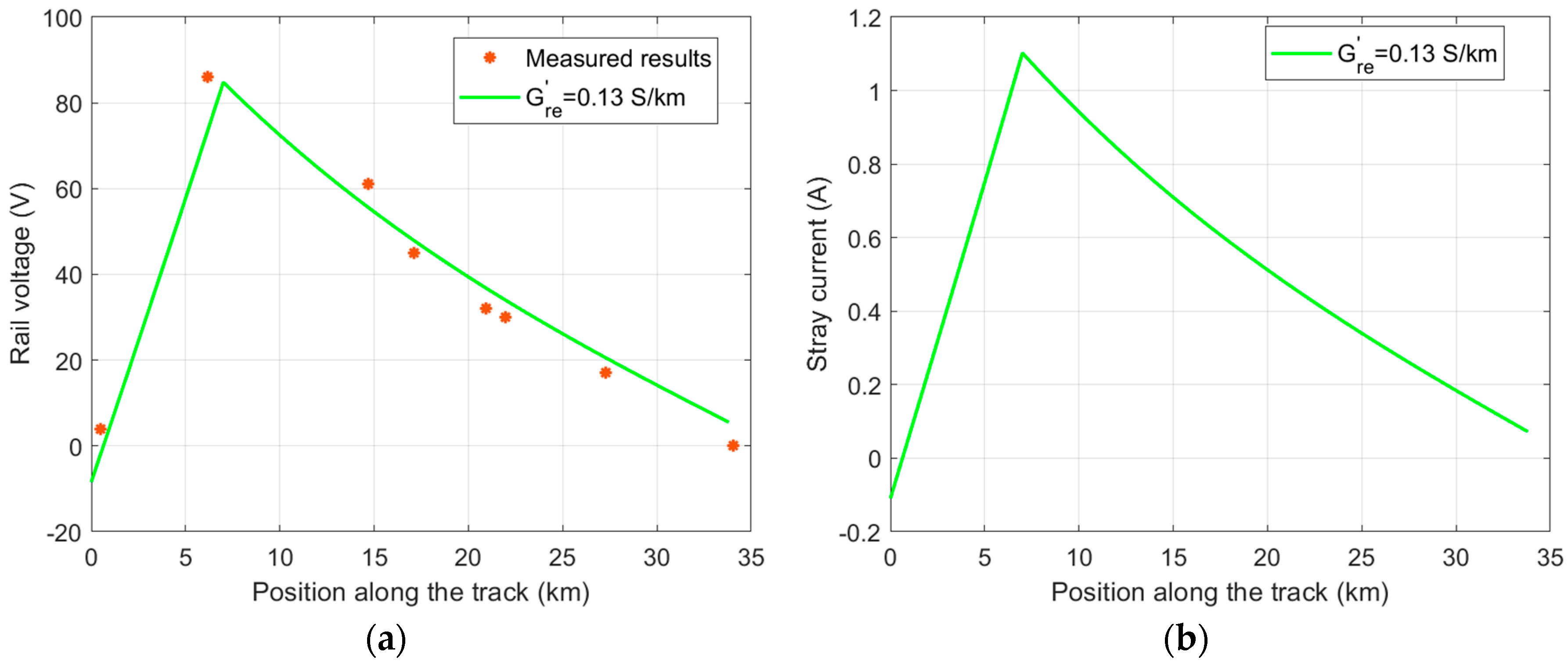
Figure 10, Figure 11 and Figure 12 show the comparison between the values of the rail voltage measured and the computed stray current along the Francavilla Fontana–Brindisi railway at different locations of the train (and different drawings of the train current I t ) with respect to those computed by the proposed model.
The agreement between measured and computed values of rail voltages in Figure 14, Figure 15 and Figure 16 is quantified in Table 4 by using the RMSE value.
The previous results show the accuracy between computed and measured results, validating the chosen circuit topology, the assumptions used for the parameters quantification, and the correctness of the practical circuit implementation inside the ADS platform. As expected, the rail voltages and the corresponding stray current have their largest amplitude when the train is around the middle of the railway section. The maximum value of the stray current reaches 1.66 A when the train is in the Latiano–Mesagne subsection, as shown in Figure 13b. Lower values are obtained in other train positions. The obtained value of the maximum stray current will be readily usable by the railway operator leading to considerations about setting spatial limits for future construction of nearby infrastructures (pipelines, industries). In the next Subsection, the same approach of comparing experimentally measured results versus those values obtained by an accurate circuit simulation is carried out on a totally different geographical scenario to better demonstrate the validity and extension of the proposed circuit approach.

3.2. Assessment of Rail Voltage and Stray Current in the S. Martino al Cimino–Capranica Railway Section

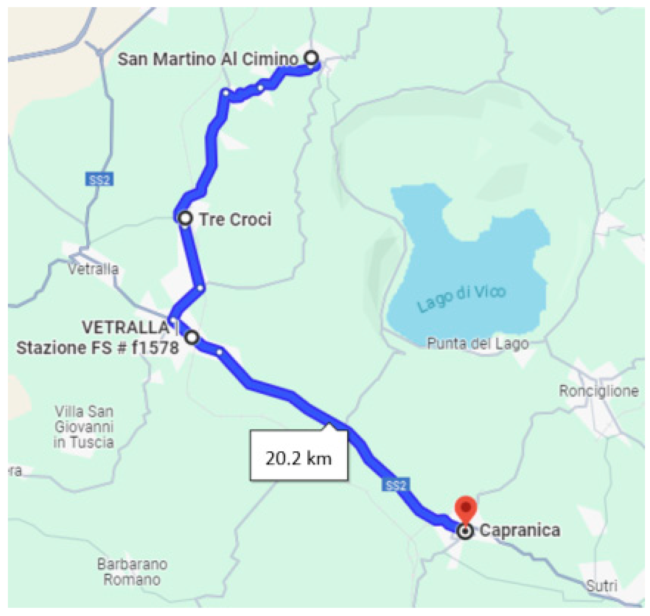
The section focuses on comparing simulation results with experimental data collected from the single-rail section between S. Martino al Cimino and Capranica whose length is 20.24 km as shown in Figure 17.
The measurement setup employed in this track is analogous to that previously described for the Francavilla Fontana–Brindisi track, and reference can be made to the description above. The circuit simulations were conducted using the key parameters specific to this track, a listed in Table 5.
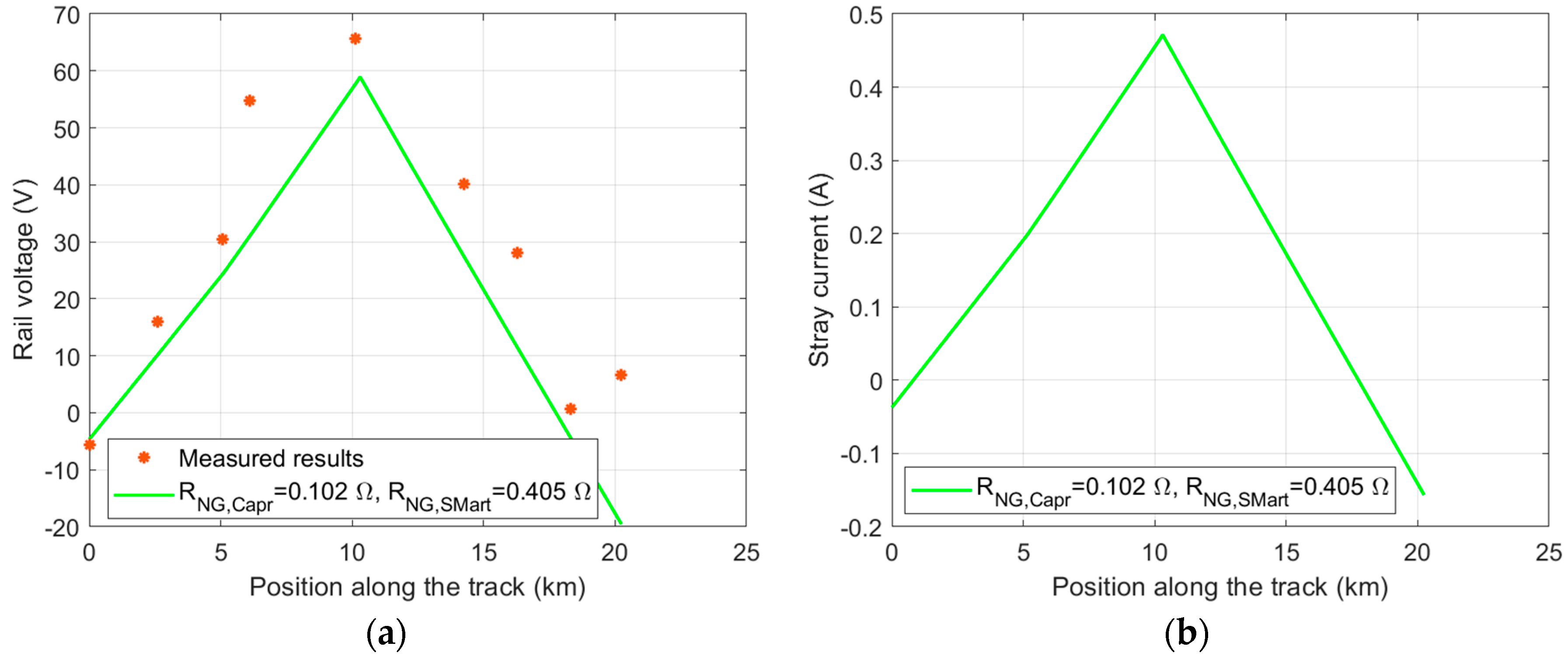
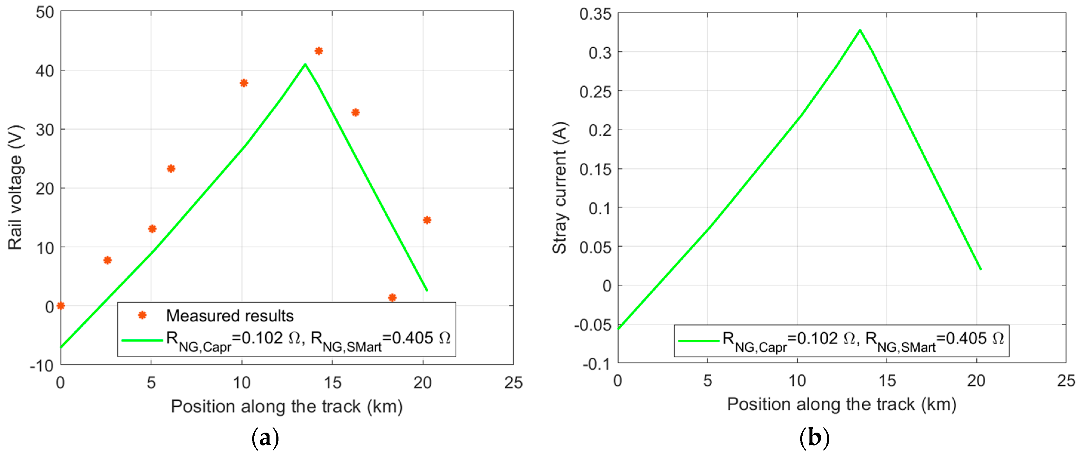
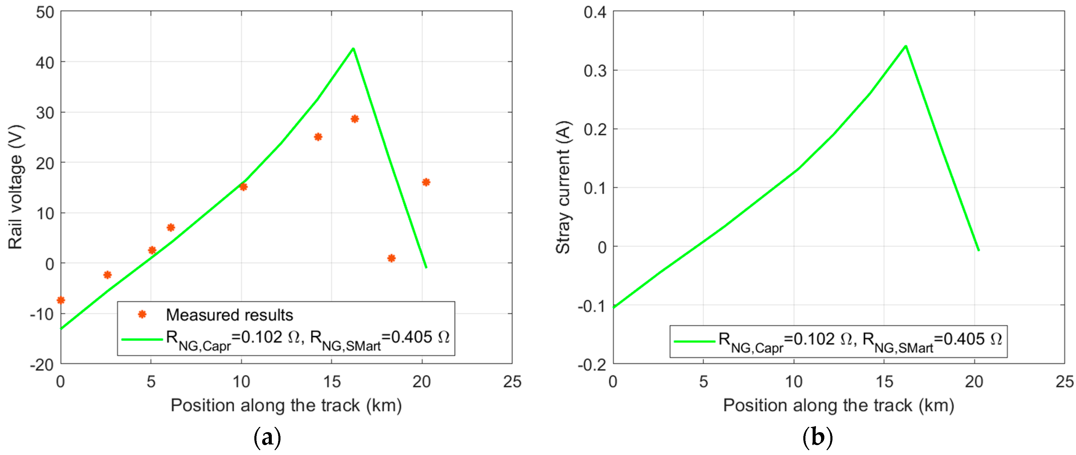
As can be observed, the G r e value used is smaller compared to the Francavilla Fontana–Brindisi section, characteristic of a terrain with less humidity (typical of this hilly section of the country) and, consequently, with better capability to mitigate stray current. For the same reasons as in the previous case of the Francavilla Fontana–Brindisi line (measurement during an active service time of the line), only one value of G r e was measured. Also, in this case the measurement was performed during permanent and constant weather conditions, allowing G r e to considered constant along the short track of the line. Notably, this section represents an intriguing case study as two different ground resistances were measured for the two substations, as detailed in the table. The study involves subdividing the rail section into three subsections: Capranica–Vetralla, Vetralla–Tre Croci, and Tre Croci–S. Martino al Cimino: for each one of these subsections, the length of the used Π-LP elementary cell is 0.1 km. The comparison between simulated and measured rail voltages (Vr) demonstrated a reasonable match, as shown in Figure 18, Figure 19 and Figure 20.
The experimental data points exhibit a clear trend, with the rail voltage peaking around the train position mark and subsequently decreasing. This pattern is consistent with the theoretical model, which shows a similar peak position and slope.
The largest error is found for the last two measurement points in Figure 18a, Figure 19a and Figure 20a toward the railway end at the TPS of San Martino al Cimino, at 18.3 km, and 20.23 km, respectively. The second-to-last point is always characterized by a very low voltage, very close to 0 V, specifically 1.7 V, 1.4 V, and 1.0 V for the three subsections Capranica–Vetralla, Vetralla–Tre Croci, and Tre Croci–San Martino al Cimino, respectively. Such points are not consistent with the expected trend indicated by the other measurement points, suggesting that measurement errors may have occurred either in the sensors or during data transfer; therefore, they are not considered reliable. A similar consideration can be made for the last point, which is characterized by a higher measured rail voltage. Aside from these two points, the agreement between the measured and computed rail voltages are consistent with each other, although larger errors are obtained (as for the point at 6.1 km) compared to the case in Section 3.1. Table 6 reports the RMSE between the measured and computed results for Figure 18, Figure 19 and Figure 20.
These latest results, along with those of the previous Section 3.1, confirm that a reduced complexity circuit model, oriented toward the evaluation of the rail voltage and the stray current itself is a viable solution for an accurate estimation of these electric variables considering the needs and constraints of the operators that must develop, to form and to use this circuit model. On the other hand, it should be noted that the visible discrepancies between measured (asterisks in the previous figures) and computed results in terms of rail voltage could stem from two different causes. On one hand, the accuracy of the measurements being performed on-field and during the in-service time of the railway are subject to more inaccuracies than those executed in a more controlled environment; on the other hand, the assumed, and in a sense also forced, assumption of a constant value of G r e becomes weaker and weaker in presence of variation in rail-to-earth interactions. Addressing these factors in future models to improve simulation accuracy and reliability, while maintaining the simplest circuit topology, is the next task.

4. Conclusions

This study demonstrates the feasibility of using reduced complexity circuit models for the prediction of rail voltages and the associated stray current itself. The knowledge of the amplitude of the stray current and its profile along the rail return path can be used for the subsequent predictive diagnostics of stray current corrosion in nearby installations. The strength of reduced complexity circuit models lies in their ability to maintain a level of accuracy that is “good enough” for most practical purposes, while drastically reducing the complexity involved. This allows operators to make quick, informed decisions without getting bogged down in the intricacies of the system they are forming and analyzing. This requirement is critical in any operative industrial environment (i.e., not strictly dedicated to research). By focusing on the most critical components and interactions within a circuit, such models streamline the process, enabling faster troubleshooting, design iterations, or performance assessments. Moreover, the ease of use makes these models accessible to a broader range of users, which can be particularly beneficial in environments where time and simplicity are key, such as in industrial applications or educational settings. Thus, simplified models provide a pragmatic tool that supports productivity without compromising the overall reliability of the analysis. This approach fosters a more efficient workflow, especially in fast-paced or resource-constrained environments.
Basically, the good agreement between simulation and measurement data highlights the relevant aspects that should be taken into account during the modeling or the testing phase of railway systems characterized by a homogeneous railway (without tunnels or viaducts) for extracting relevant design and safety information from the computed rail voltage and the stray current.
Although more complex circuit modeling could potentially provide a more accurate prediction of the stray current, the knowledge of the order of magnitude of such a stray current allows the rail designer to make an initial decision on the relative position between the rail track and potential victims such as pipelines and grounding circuits for nearby industries and power systems. A more precise calculation of the stray current along the rail track could be of greater interest, especially inside tunnels, where layered ground made with iron-reinforced concrete and insulation layers may largely affect the stray current path conductance. This will be the objective of future work aimed at providing a general circuit for modeling complex terrains.
For such cases, based on the current findings and possible discrepancies due to the G′re variation along the rail track, further investigation is planned with on-field evaluation of multiple G′re points after carefully analyzing the underground and geological profile. This information and data will be available from the more recent railway designs and the installation of the railway track to be analyzed in the near future.
Moreover, based on this initial work and the verification of the applicability of this simple circuit model, a subsequent work is planned for the near future for analyzing railway scenarios involving both tunnels and viaducts, thus not being able to consider a single conductance value as performed herein.

Author Contributions

Data Curation, F.d.P. and F.S.; Funding acquisition, M.C.; Investigation, C.O. and A.O.; Methodology, F.d.P. and F.S.; Project administration, F.S.; Resources, M.C.; Supervision, A.O. and M.C.; Visualization, L.D.L.; Writing—original draft, L.D.L. and A.O.; Writing—review & editing, C.O. and L.D.L. All authors have read and agreed to the published version of the manuscript.

Funding

This research received no external funding.

Data Availability Statement

The datasets presented in this article are not readily available because the Authors do not have the permission to distribute the data.

Conflicts of Interest

The Authors declare that they have no conflicts of interest.

References

  1. Regula, M.; Siranec, M.; Otcenasova, A.; Hoger, M. Possibilities of the stray current measurement and corrosive risk evaluation. Electr. Eng. 2022, 104, 2497–2513. [Google Scholar] [CrossRef]
  2. Siranec, M.; Regula, M.; Otcenasova, A.; Altus, J. Measurement and Evaluation of the Stray Currents from the DC Electric Traction Systems. In Proceedings of the 2020 ELEKTRO, Taormina, Italy, 25–28 May 2020; pp. 1–6. [Google Scholar] [CrossRef]
  3. Höger, M.; Reguľa, M.; Roch, M. Investigating the impacts of high voltage powerlines on ground current fields. Transp. Res. Procedia 2023, 74, 900–907. [Google Scholar] [CrossRef]
  4. Aatif, S.; Hu, H.; Rafiq, F.; He, Z. Analysis of rail potential and stray current in MVDC railway electrification system. Railw. Eng. Sci. 2021, 29, 394–407. [Google Scholar] [CrossRef]
  5. Wieczorek, G.; Bernacki, K.; Rymarski, Z.; Oliwa, W. Gathering Energy of the Stray Currents in Electrified Railways Environment for Power Supply. Energies 2021, 14, 6206. [Google Scholar] [CrossRef]
  6. Mariscotti, A. Stray Current Protection and Monitoring Systems: Characteristic Quantities, Assessment of Performance and Verification. Sensors 2020, 20, 6610. [Google Scholar] [CrossRef] [PubMed]
  7. Charalambous, C.A.; Cotton, I.; Aylott, P. A Simulation Tool to Predict the Impact of Soil Topologies on Coupling Between a Light Rail System and Buried Third-Party Infrastructure. IEEE Trans. Veh. Technol. 2008, 57, 1404–1416. [Google Scholar] [CrossRef]
  8. Chen, L.; Zhang, B.; Wei, K.; Fang, D.; Zou, Q. Analysis of Leakage Current Characteristics of Rail Insulation Fasteners Based on ANSYS. In Proceedings of the 2021 IEEE Sustainable Power and Energy Conference (iSPEC), Nanjing, China, 23–25 December 2021; pp. 2640–2643. [Google Scholar] [CrossRef]
  9. Zaboli, A.; Vahidi, B.; Yousefi, S.; Hosseini-Biyouki, M.M. Evaluation and Control of Stray Current in DC-Electrified Railway Systems. IEEE Trans. Veh. Technol. 2017, 66, 974–980. [Google Scholar] [CrossRef]
  10. Huang, K.; Lin, G.; Liu, Z. Prediction Approach of Negative Rail Potentials and Stray Currents in Medium-Low-Speed Maglev. IEEE Trans. Transp. Electrif. 2022, 8, 3801–3815. [Google Scholar] [CrossRef]
  11. Liu, W.; Li, T.; Jie, Z.; Weiguo, P.; Yichen, Y. Evaluation of the Effect of Stray Current Collection System in DC-Electrified Railway System. IEEE Trans. Veh. Technol. 2021, 70, 6542–6553. [Google Scholar] [CrossRef]
  12. Zhu, C.; Zheng, Z.; Du, G.; Hu, J.; Kang, C.; Hu, J.; Yang, Y. Simulation Method of DC Traction Power Systems with Complex Operation Conditions Based on Unified Chain Model. In Proceedings of the 2020 IEEE 9th International Power Electronics and Motion Control Conference (IPEMC2020-ECCE Asia), Nanjing, China, 29 November–2 December 2020; pp. 846–852. [Google Scholar] [CrossRef]
  13. Jamali, S.; Alamuti, M.M.; Savaghebi, M. Effects of different earthing schemes on the stray current in rail transit systems. In Proceedings of the 2008 43rd International Universities Power Engineering Conference, Padua, Italy, 1–4 September 2008; pp. 1–5. [Google Scholar] [CrossRef]
  14. Fichera, F.; Mariscotti, A.; Ogunsola, A.; Sandrolini, L. Comparison of distributed and lumped parameters stray current models. In Proceedings of the 2013 Africon, Pointe aux Piments, Mauritius, 9–12 September 2013; pp. 1–5. [Google Scholar] [CrossRef]
  15. Li, C.; Du, Q.; Guo, Y.; Liu, Y.; Yang, F.; Chen, L.; Zhang, X.; Huang, G.; Gao, G.; Wu, G. Modeling of Stray Currents from Metro Intruding into Power System Considering the Complex Geological Conditions in Modern Megacities. IEEE Trans. Transp. Electrif. 2023, 9, 1653–1663. [Google Scholar] [CrossRef]
  16. Tang, M.; Zhong, H.; Zhu, T.; Zhang, J.; Yan, J.; Xiao, S.; Guo, Y.; Wu, G. The Distribution Analysis of the Ground Potential and Stray Current in Power Grid Under the Operation of Metro System. In Proceedings of the 2023 2nd International Conference on Power Systems and Electrical Technology (PSET), Milan, Italy, 25–27 August 2023; pp. 158–162. [Google Scholar] [CrossRef]
  17. Zhou, Q.; Lin, S.; Lin, X.; Wang, A. A Uniform Model for Stray Current of Long-Line DC Metro Systems. IEEE Trans. Transp. Electrif. 2022, 8, 2915–2927. [Google Scholar] [CrossRef]
  18. Wang, C.; Li, W.; Wang, Y.; Xu, S.; Fan, M. Stray Current Distributing Model in the Subway System: A review and outlook. Int. J. Electrochem. Sci. 2018, 13, 1700–1727. [Google Scholar] [CrossRef]
  19. Arboleya, P.; Mayet, C.; Mohamed, B.; Aguado, J.A.; de la Torre, S. A review of railway feeding infrastructures: Mathematical models for planning and operation. eTransportation 2020, 5, 100063. [Google Scholar] [CrossRef]
  20. Tzeng, Y.-S.; Lee, C.-H. Analysis of Rail Potential and Stray Currents in a Direct-Current Transit System. IEEE Trans. Power Deliv. 2010, 25, 1516–1525. [Google Scholar] [CrossRef]
  21. Ogunsola, A.; Sandrolini, L.; Mariscotti, A. Evaluation of Stray Current From a DC-Electrified Railway with Integrated Electric–Electromechanical Modeling and Traffic Simulation. IEEE Trans. Ind. Appl. 2015, 51, 5431–5441. [Google Scholar] [CrossRef]
  22. Vranešić, K.; Haladin, I.; Lakušić, S.; Burnać, K. Convenient Procedure for Measuring the Electrical Resistance of Fastening Systems in Urban Railway Tracks. Energies 2023, 16, 1990. [Google Scholar] [CrossRef]
  23. Bhagat, S.; Bongiorno, J.; Mariscotti, A. Uncertainty of Standardized Track Insulation Measurement Methods for Stray Current Assessment. Sensors 2023, 23, 5900. [Google Scholar] [CrossRef] [PubMed]
  24. Ku, B.-Y. Rail-to-Earth Resistance Assessment: A Medium Capacity Transit System with Continuous Negative Rails by Potential Measurement. IEEE Veh. Technol. Mag. 2016, 11, 29–35. [Google Scholar] [CrossRef]
  25. Alamuti, M.; Nouri, H.; Jamali, S. Effects of earthing systems on stray current for corrosion and safety behaviour in practical metro systems. IET Electr. Syst. Transp. 2011, 1, 69–79. [Google Scholar] [CrossRef]
  26. Liu, N.; Du, G.; He, F.; Li, Q.; Xu, F.; Huang, W.; Jiang, X.; Zhu, Z. Optimization of grounding resistance in multitrain DC subway system based on MOEA/D-DE. IET Intell. Transp. Syst. 2023, 17, 1675–1689. [Google Scholar] [CrossRef]
  27. Chuchit, T.; Kulworawanichpong, T. Stray current assessment for DC transit systems based on modelling of earthing and bonding. Electr. Eng. 2019, 101, 81–90. [Google Scholar] [CrossRef]
  28. Soylemez, M.T.; Acikbas, S.; Kaypmaz, A. Controlling rail potential of DC supplied rail traction systems. Turk. J. Electr. Eng. 2006, 14, 475–484. [Google Scholar]
  29. Keysight Pathwave Advanced Design System, ADS 2023. Available online: https://www.keysight.com/us/en/products/software/pathwave-design-software/pathwave-advanced-design-system.html (accessed on 2 December 2022).
  30. EN 50122-1:2022; Railway Applications—Fixed Installations—Electrical Safety, Earthing and the Return Circuit—Part 1: Protective Provisions Against Electric Shock. CENELEC: Brussels, Belgium, 2022.
  31. EN 50122-2:2022; Railway Applications—Fixed Installations—Electrical Safety, Earthing and the Return Circuit—Part 2: Provisions Against the Effects of Stray Current Caused by DC Traction Systems. CENELEC: Brussels, Belgium, 2022.
  32. EN 50163:2022; Railway Applications—Supply Voltages of Traction Systems. CENELEC: Brussels, Belgium, 2022.
  33. Fluke. A3003 FC, Operating Manual; Fluke: Everett, WA, USA, 2024. [Google Scholar]
  34. Fluke. V3001AC, Operating Manual; Fluke: Everett, WA, USA, 2023. [Google Scholar]
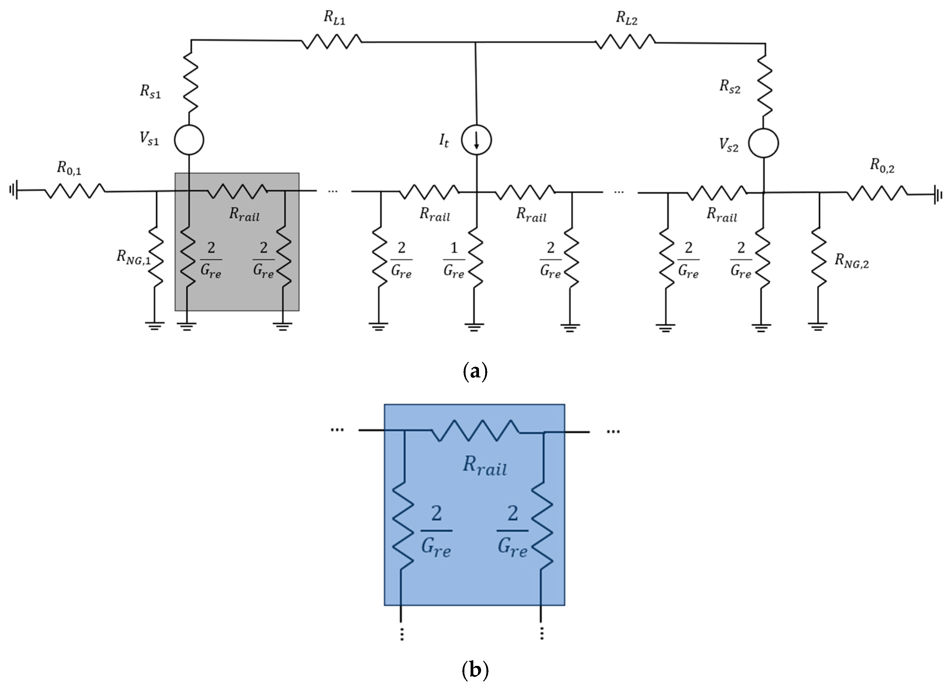
Figure 1. (a) The circuit employed for the modeling of a DC railway traction system oriented to the evaluation of Vr and stray current. In the highlighted box, the elementary Π cell. (b) The elementary Π cell of the circuit employed for the modeling of a DC railway traction system oriented to the evaluation of Vr and stray current.
Electronics 14 04541 g001
Figure 2. Circuit modeling of the grounding of substations in railway systems. In the highlighted box there is the equivalent negative pole-to-ground resistance for the TPS.
Electronics 14 04541 g002
Figure 3. Modeling of the running rails adjacent (i.e., downstream) to the railway segment under study. The selected rectangle shows the equivalent resistance of the running rails upstream of the railway segment.
Electronics 14 04541 g003
Figure 4. Geographical view of the Francavilla Fontana–Brindisi railway (Google, 2024).
Electronics 14 04541 g004
Figure 5. Electric traction schematic of the Francavilla Fontana–Brindisi railway.
Electronics 14 04541 g005
Figure 6. Details of installed instrumentation and data acquisition system at Brindisi TPS: (a) Optical link to transfer data; (b) LEM/LV-4000 SP6.
Electronics 14 04541 g006
Figure 7. Details of the installed instrumentation and data acquisition system in the Mesagne Ovest TE return circuit: (a) current clamp on the longitudinal connection; (b) voltmeter connection between the return circuit and the reference electrode.
Electronics 14 04541 g007
Figure 8. The ADS implementation of the circuit employed for the modeling of a Francavilla Fontana–Brindisi railway section using a spatial grid of 0.1 km: (a) focus on the Francavilla Fontana TPS and simulation parameters; (b) focus on the train source current in position 29.8 km; (c) subcircuit of the elementary Π−LP cell.
Electronics 14 04541 g008
Figure 9. Spatial distribution of the rail voltage and stray current with train position in the Latiano–Mesagne section and train current It = 1217 A: (a) rail voltage; (b) stray current. In (a), to quantify the accuracy between the measured (red asterisks) and computed results (labeled “Model w/ G r e = 0.13 S/km, w/RNG”) the root-mean-square error (RMSE) between these two sets of data was computed to be 3.34 V.
Electronics 14 04541 g009
Figure 10. Spatial distribution of the rail voltage for measured and computed results with different lengths of the elementary cells, with train position in the Latiano–Mesagne subsection and train current It = 1217 A.
Electronics 14 04541 g010
Figure 11. Ten sets of G r e (one value per km) obtained by ten random Gaussian distributions (r.d.) with mean equal to the measured value of G r e (0.13 S/km) and a standard deviation σ = 30% of the mean value added.
Electronics 14 04541 g011
Figure 12. Spatial distribution of the rail voltage and differences in ten cases of G r e = 0.13 S/km with a random Gaussian distribution (r.d.) and a standard deviation σ = 30% of the mean value added, considering a train position in the Latiano–Mesagne subsection and train current It = 1217 A: (a) rail voltage; (b) rail voltage differences.
Electronics 14 04541 g012aElectronics 14 04541 g012b
Figure 13. Spatial distribution of the rail voltage and stray current in three cases: R N G , n = 0.017 Ω, R N G , a = 1.5, R N G , n = 0.0255 Ω, and R N G , b = 0.5, R N G , n = 0.0085 Ω, considering a train position in the Latiano–Mesagne subsection and train current It = 1217 A: (a) rail voltage; (b) stray current.
Electronics 14 04541 g013
Figure 14. Spatial distribution of the rail voltage and stray current with train position in the Mesagne–Brindisi subsection and train current It = 1190 A: (a) rail voltage; (b) stray current.
Electronics 14 04541 g014
Figure 15. Spatial distribution of the rail voltage and stray current with train position in the Oria–Latiano subsection and train current It = 1272 A: (a) rail voltage; (b) stray current.
Electronics 14 04541 g015
Figure 16. Spatial distribution of the rail voltage and stray current with train position in the Francavilla Fontana–Oria subsection and train current It = 1202 A: (a) rail voltage; (b) stray current.
Electronics 14 04541 g016
Figure 17. Geographical view of the S. Martino al Cimino–Capranica railway (Google, 2024).
Electronics 14 04541 g017
Figure 18. Spatial distribution of the rail voltage and stray current with train position in the—Capranica–Vetralla subsection and train current It = 1049.4 A: (a) rail voltage; (b) stray current.
Electronics 14 04541 g018
Figure 19. Spatial distribution of the rail voltage and stray current with train position in the Vetralla–Tre Croci subsection and train current It = 670.5 A: (a) rail voltage; (b) stray current.
Electronics 14 04541 g019
Figure 20. Spatial distribution of the rail voltage and stray current with train position in the Tre Croci–San Martino al Cimino subsection and train current It = 1137 A: (a) rail voltage; (b) stray current.
Electronics 14 04541 g020
Table 1. Nominal parameters of the Francavilla Fontana–Brindisi Railway.
QuantitySymbolValueUnit
TPS source voltages V S   ( V S 1   =   V S 2 )3500V
TPS internal resistance R S   ( R S 1   =   R S 2 )0.15Ω
Longitudinal resistance of the contact line per kilometer R L 0.0415Ω/km
Resistance of the rail per kilometer R r a i l 0.015Ω/km
Conductance of the rail per kilometer G r e 0.13S/km
Termination resistance R 0 ( R 0,1     R 0,2 ) 0.34Ω
Neutral-to-ground resistance TPS R N G ( R N G , 1     R N G , 2 ) 0.017Ω
Table 2. Substation rail voltages in case of R N G , n = 0.017 Ω, R N G , a = 1.5, R N G , n = 0.0255 Ω, and R N G , b = 0.5, R N G , n = 0.0085 Ω, considering a train position in the Latiano–Mesagne subsection and train current It = 1217 A.
R N G (Ω)Rail Voltage at Francavilla Fontana Substation (0 km)
(V)
Rail Voltage at Brindisi Substation (33.8 km)
(V)
0.017   ( R N G , n )−7.423.14
0.0255   ( R N G , a )−10.44.21
0.0085   ( R N G , b )−4.001.78
Table 3. Substations stray current in case of R N G , n = 0.017 Ω, R N G , a = 1.5 R N G , n = 0.0255 Ω, and R N G , b = 0.5, R N G , n = 0.0085 Ω, considering a train position in the Latiano–Mesagne subsection and train current It =1217 A.
R N G
(Ω)
Stray Current at Francavilla Fontana Substation (0 km)
(A)
Stray Current at Brindisi Substation (33.8 km)
(A)
0.017   ( R N G , n )−0.0960.041
0.0255   ( R N G , a ) −0.130.054
0.0085   ( R N G , b )−0.0520.023
Table 4. RMSE for the subsections of the e Francavilla Fontana–Brindisi railway.
Subsection—FigureRMSE (V)
Mesagne–Brindisi—Figure 144.39
Oria–Latiano—Figure 157.90
Francavilla Fontana–Oria—Figure 166.09
Table 5. Nominal parameters of the S. Martino al Cimino–Capranica Railway.
QuantitySymbolValueUnit
TPS Source voltages V S   ( V S 1   =     V S 2 )3500V
TPS internal resistance R S   ( R S 1   =   R S 2 )0.15Ω
Longitudinal resistance of the contact line per kilometer R L 0.05725Ω/km
Resistance of the rail per kilometer R r a i l 0.015Ω/km
Conductance of the rail per kilometer G r e 0.08S/km
Termination resistance R 0 ( R 0,1 = R 0,2 ) 0.43Ω
Neutral-to-ground resistance TPS Capranica R N G , C a p r 0.017Ω
Neutral-to-ground resistance TPS S. Martino Al Cimino R N G , S M a r t 0.450Ω
Table 6. RMSE for the subsections of the San Martino al Cimino–Capranica Railway.
Subsection—FigureRMSE (V)
Capranica–Vetralla—Figure 1814.32
Vetralla–Tre Croci—Figure 198.98
Tre Croci–San Martino al Cimino—Figure 2010.11
Disclaimer/Publisher’s Note: The statements, opinions and data contained in all publications are solely those of the individual author(s) and contributor(s) and not of MDPI and/or the editor(s). MDPI and/or the editor(s) disclaim responsibility for any injury to people or property resulting from any ideas, methods, instructions or products referred to in the content.