Abstract
Few-shot fault diagnosis (FSFD) seeks to build accurate models from scarce labeled data, a frequent challenge in industrial settings with noisy measurements and varying operating conditions. Conventional metric-based meta-learning (MBML) often assumes task-invariant, class-separable feature spaces, which rarely hold in heterogeneous environments. To address this, we propose a Transformer-embedded Task-Adaptive-Regularized Prototypical Network (TETARPN). A tailored Transformer-based Temporal Encoder Module is integrated into MBML to capture long-range dependencies and global temporal correlations in industrial time series. In parallel, a task-adaptive prototype regularization dynamically adjusts constraints according to task difficulty, enhancing intra-class compactness and inter-class separability. This combination improves both adaptability and robustness in FSFD. Experiments on bearing benchmark datasets show that TETARPN consistently outperforms state-of-the-art methods under diverse fault types and operating conditions, demonstrating its effectiveness and potential for real-world deployment.
1. Introduction
Fault diagnosis serves as a cornerstone in maintaining the operational stability and safety of industrial systems [1,2]. With the increasing popularity of monitoring sensors and data acquisition equipment, abundant sensor data has made condition monitoring more feasible [3], which has aroused widespread interest among experts and scholars in adopting data-driven fault diagnosis methods [4].
Among the prevailing data-driven strategies for fault diagnosis, learning-based methods have become the mainstream due to their ability to automatically extract discriminative features from complex, high-dimensional sensor data [5]. For example, Zuo et al. proposed extraction networks and dual-model geometric calibration to monitor the status of bolts in industrial magnetic separation systems [6]; Mukherjee et al. developed deep learning models to detect pipeline faults from sensor data [7]; Cheng et al. trained a physics-informed Fourier neural operator as a surrogate solver for pantograph–catenary dynamics [8]; Chen et al. developed a parallel attention module within a flexible residual structure, showing improved diagnostic accuracy under noisy conditions [9]; Chen et al. proposed a multi-scale ScConv and quaternion Transformer method based on a hybrid attention mechanism for noise-resistant bearing fault diagnosis [10]. These models eliminate the need for hand-crafted feature design and offer scalable solutions across diverse equipment types and operating conditions [11]. In laboratory settings or data-rich environments, such methods have shown remarkable accuracy and robustness, fueling their rapid adoption in predictive maintenance and intelligent monitoring systems [12]. Nevertheless, translating these successes to real-world applications presents persistent challenges [13]. Fault data, by nature, are difficult to obtain in sufficient quantity and diversity, often limited to a few cases captured under specific conditions [14]. Therefore, defining fault diagnosis as a few-shot learning problem is more in line with real-world requirements [15].
This paradigm is fundamentally more challenging than traditional data-driven approaches for several reasons. First, while conventional methods excel in data-rich environments, they struggle to generalize from the limited samples available in real-world industrial settings, where fault events are inherently rare. Second, the process of labeling fault data requires costly and time-consuming manual inspection by domain experts, making the creation of large-scale labeled datasets infeasible. Therefore, few-shot fault diagnosis (FSFD) directly confronts these practical constraints by aiming to build robust models from inherently scarce data, a scenario where traditional methods often fall short.
To address the challenges of FSFD, three mainstream solutions have emerged: domain generalization, self-supervised learning, and meta-learning. Domain generalization enhances cross-domain adaptability by learning invariant features from multiple source domains, reducing reliance on target-specific data [16]. For instance, Li et al. first demonstrated this principle by adversarially aligning feature distributions in four source domains [17]. Self-supervised learning leverages intrinsic data structures to generate pseudo-labels, addressing annotation scarcity through contrastive learning or auxiliary tasks [18]. For example, Fu et al. proposed a self-supervised learning approach for time-series anomaly detection, which was the first attempt to apply masked self-supervised learning to multivariate time-series anomaly detection [19]. Lastly, meta-learning explicitly models how to learn from a few instances across multiple tasks. Furthermore, meta-learning introduces a highly adaptive learning paradigm that addresses the few-shot problem by focusing on the acquisition of learning capabilities rather than just learning itself [20]. Therefore, meta-learning-based fault diagnosis has gradually become a potential solution for FSFD [21].
In the meta-learning paradigm, it is generally assumed that knowledge acquired from multiple auxiliary fault diagnosis tasks can be leveraged to rapidly adapt to new, related tasks with scarce labeled samples. The goal is to build a diagnosis model that can swiftly generalize to unseen fault conditions with minimal fine-tuning effort. In recent years, increasing attention has been paid to the application of optimization-based meta-learning algorithms in the FSFD domain. For instance, a first-order approximation of model agnostic meta-learning (MAML) was employed to reduce training complexity while maintaining adaptation efficiency in mechanical fault diagnosis scenarios [20]; another line of work proposed a meta-regularization framework to constrain parameter updates and enhance generalization in noisy industrial environments [22]; additionally, a hybrid meta-learning model combining task-specific adaptation and shared representation learning was designed for cross-domain fault identification [23]. These methods typically aim to establish a set of initialization parameters that are broadly optimal across tasks, thereby enabling efficient adaptation to target fault types using few labeled examples. However, when the task distribution is highly heterogeneous, these approaches may struggle to maintain stable convergence and generalization performance [24]. Striking an effective balance between rapid adaptability and model stability thus remains a critical challenge for practical deployment.
In contrast, metric-based meta-learning (MBML) has demonstrated strong robustness in FSFD scenarios, particularly under low-data conditions where task heterogeneity and label scarcity can hinder optimization-based approaches. By learning an embedding space in which intra-class features are compact and inter-class features are well separated, MBML shifts the adaptation burden from parameter fine-tuning to metric computation, thereby improving stability and reducing overfitting risk [25,26]. Among MBML methods, prototypical networks (PNs) [25] remain a widely adopted and conceptually simple baseline; however, their effectiveness in realistic FSFD is constrained by implicit assumptions of class-separable and task-invariant embeddings, which are often violated under non-stationary conditions, sensor noise, and severe class imbalance.
To mitigate these PN limitations, recent studies have explored diverse strategies, including PN with center loss (PN-CL) [27] and PN with center triplet loss (PN-CTL) [28]. They use different loss function constraints to make similar samples more focused and different samples separated. In addition, conductive inference, distribution calibration, or cross-domain alignment can be used to alleviate distribution shift [29,30]. While methods like PN-CL and PN-CTL have improved performance by refining the loss function to better structure the embedding space, they often rely on conventional encoders that struggle with long-range temporal dependencies and employ static regularization constraints. Two key challenges remain underexplored in FSFD: the lack of strong temporal embeddings capable of modeling long-range dependencies under noisy industrial time series and the absence of task-difficulty-aware regularization that adapts prototype geometry to varying episodic complexities. Recent studies have explored Transformer-based variants for industrial fault diagnosis and reported promising results, which motivates us to further investigate their potential for capturing temporal dependencies in complex industrial data [31,32].
To address the challenges of effectively modeling long-range temporal dependencies in noisy industrial time series and adapting prototype representations to varying task difficulties, we propose a novel framework termed transformer-embedded Task-Adaptive-Regularized Prototypical Network (TETARPN). Unlike conventional approaches relying on convolutional encoders, TETARPN leverages the powerful self-attention mechanism of the Transformer to extract richer and more robust feature embeddings that better capture temporal context and subtle fault characteristics. Meanwhile, a task-adaptive prototype regularization strategy is introduced to dynamically guide the prototype learning process according to the complexity of each diagnostic task, encouraging more compact intra-class distributions and clearer inter-class boundaries. By jointly integrating these components, our method aims to significantly enhance the generalization capability and diagnostic accuracy in few-shot fault diagnosis scenarios under realistic industrial conditions.
The main contribution of this article is summarized as follows.
- 1.
- To overcome the limitations of conventional encoders in modeling complex industrial signals, we design a Transformer-based Temporal Encoder (TBTE). This module adapts the self-attention mechanism to tokenize time series into segments, enabling it to capture not only local dynamics but also critical long-range temporal dependencies. This results in more discriminative feature embeddings crucial for distinguishing subtle fault characteristics.
- 2.
- We propose a novel Task-Adaptive Prototype Regularization (TAPR) strategy to address the challenge of task heterogeneity. This mechanism dynamically adjusts the regularization strength based on the difficulty of each few-shot task, promoting more compact intra-class distributions and clearer inter-class boundaries. This enhances the model’s adaptability and robustness in diverse and challenging diagnostic scenarios.
The rolling bearing benchmark are used to analyze the FSFD performance of the proposed TETARPN approach. Extensive experiments demonstrate its effectiveness and superiority in comparison with state-of-the-art methodologies.
2. Preliminary
2.1. Problem Formulation
In practical industrial environments, it is often possible to pre-identify various system states—such as normal operations or fault conditions—through domain knowledge and prior experience [33]. Based on this insight, we consider a scenario where data samples are collected under M known operating conditions, forming a labeled dataset , where each input denotes a p-dimensional measurement, and each label indicates its corresponding condition category. These samples are naturally grouped in the joint space , aligning with different machine states. Traditionally, the goal of fault diagnosis is cast as a multi-class classification problem, in which a model is trained to accurately distinguish between these pre-defined categories [5].
However, in real-world industrial applications, obtaining a sufficient amount of labeled faulty data remains a significant bottleneck. It should be noted that the general consensus on “few shot” usually refers to scenarios where each category contains only a very limited number of samples. Not only that, fault events are rare by nature, and their labeling often requires costly manual inspection or domain expertise, making large-scale data acquisition infeasible. This limitation challenges the effectiveness of conventional supervised learning methods, especially when faced with limited samples for new fault types [34]. To address this issue, our study explores a more realistic and challenging FSFD scenario. In particular, we adopt the MBML approach, which is designed to emulate the adaptive behavior of experienced engineers: leveraging accumulated knowledge from past fault scenarios to quickly generalize to new, data-scarce diagnostic tasks.
2.2. Fault Diagnosis Based on PN
Fault diagnosis in industrial systems often suffers from insufficient labeled data under new or rare fault conditions, making it challenging for conventional supervised classifiers to generalize effectively. PN offers a compact yet powerful framework to address this challenge by learning a metric space where classification can be performed by computing distances to class prototypes. In this way, PN naturally supports rapid adaptation to unseen fault types with only a few labeled samples, a capability that is particularly valuable for real-world diagnostic scenarios. The method employs an episodic training strategy, which mimics the human ability to quickly adapt to new fault scenarios by leveraging prior knowledge [35]. The core idea is to learn an embedding that pulls together instances from the same class while pushing apart those from different classes, thereby facilitating generalization to novel working conditions not encountered during training [36].
To realize this idea, PN constructs a large number of small, structured classification tasks—also referred to as episodes—during training. Let us denote the set of these episodes as , each sampled from an overall dataset . Each episode contains labeled instances for to , which are divided into two mutually exclusive subsets: the support set and the query set . A typical configuration involves selecting K examples per class for the support set, covering M distinct classes, commonly referred to as an “M-way K-shot” setting. Here, denotes the total number of support samples in each episode. The remaining samples from each class are reserved for the query set, which is used to evaluate the model’s generalization capability within the episode [26].
The architecture of PN generally comprises two main modules: a feature extraction module and a prototype-based classification mechanism [35]. The feature extractor maps raw input data into a latent space , parameterized by . This mapping can be instantiated via various neural network backbones, such as 1-D convolutional networks tailored to vibration signal analysis in rotating machinery [37]. Once embedded, samples from the same class in the support set are aggregated to define a class prototype. Typically, this prototype is computed by averaging the embedded representations:
where denotes the subset of support samples belonging to class m, and is the input sample. The key insight of this approach is that even with a very small number of support samples (K-shot), this mean vector can serve as a robust estimator for the class centroid in the learned embedding space.
For classification, the model compares the embedding of each query sample with the stored prototypes. In PN [25], similarity is measured using the squared Euclidean distance, denoted as , and the probability of a query sample belonging to class m is given by
The model parameters are trained to minimize the cross-entropy loss over the predictions on the query set:
What sets PN apart from standard training regimes is its episodic nature. Specifically, during each training iteration, a new episode is randomly sampled, a fresh support set is used to generate prototypes, and the model is updated based on its performance over the query set. This episodic loop is repeated over diverse training episodes, enabling the model to internalize a general strategy for fast adaptation. Once training concludes, the model is deployed on an unseen target episode , where a few labeled instances are used to form new prototypes, and the remaining is used to assess diagnostic performance under the few-shot setting in the target domain. It must be stated that, unlike KTR-BUNN [38], which characterizes class prototypes by constructing fault knowledge graphs to enhance intra-class compactness and inter-class separability, and introduces new categories explicitly through a triple-tier unknown fault separator, PN defines prototypes as the mean embedding of a few labeled instances within each episode. Consequently, PN enables accurate feature representation from small samples and can adapt to novel categories, but relies on distance thresholds for unknown detection rather than explicitly modeling the separation of unseen faults.
3. Fault Diagnosis Based on TETARPN
3.1. Overview of the Proposed Method
Although PN and its variants have demonstrated strong capability in MBML-based FSFD, their performance can still be hindered by two key limitations. First, PN-based methods’ embedding modules, typically based on shallow or convolutional architectures, are insufficient for capturing long-range temporal dependencies inherent in sequential signals. Second, they often struggle to cope with substantial task variability, which can lead to unstable feature distributions across different tasks.
To address the challenges of long-range temporal dependency and task variability, we propose a general-purpose framework named Transformer-embedded Task-Adaptive-Regularized Prototypical Network (TETARPN). This framework seamlessly integrates two complementary enhancements into the conventional PN structure: a Transformer-based Temporal Encoder (TBTE) tailored for time series and a Task-Adaptive Prototype Regularization (TAPR) mechanism, as shown in Figure 1. The framework’s workflow proceeds as follows: First, each task’s data is divided into a support set and a query set. Both sets are processed by the Transformer-based Temporal Encoder to extract powerful temporal features. For the support set, these features are then used to compute class prototypes. Concurrently, the Task-Adaptive Regularization Module calculates a regularization loss that encourages intra-class compactness and inter-class separability. This loss is dynamically weighted based on the task’s initial difficulty and is combined with the primary classification loss from the query set to form a comprehensive task loss, which guides the model’s optimization.
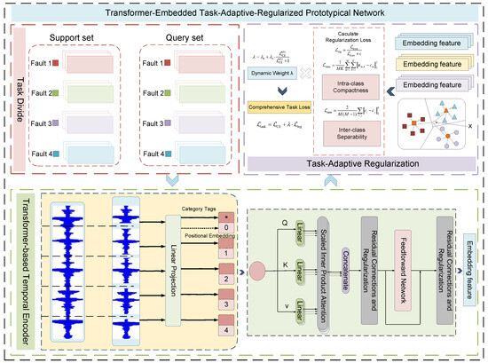
Figure 1.
The framework of the proposed TETARPN method.
The first component of TETARPN is the TBTE module, which serves as a high-capacity embedding function for time series. Traditional CNN or LSTM-based encoders struggle to capture global temporal features due to local receptive field limitations or sequential processing bottlenecks. In contrast, our embedding module utilizes a self-attention mechanism with positional encoding to extract long-term dependencies across time steps. To better adapt the Transformer to fault diagnosis scenarios, we adopt a time-series segmentation strategy as preprocessing, which partitions complex signals into meaningful intervals, enabling the attention mechanism to focus on discriminative temporal patterns.
The second component is the TAPR module, designed to dynamically adapt to the difficulty of each individual few-shot task. Unlike conventional PNs that optimize uniformly across tasks, this module computes an intra-class and inter-class prototype loss and adjusts its contribution according to the initial task loss. This allows the model to maintain compact intra-class distributions while enhancing inter-class separability, thereby improving generalization under varying task complexities.
By combining these two components, TETARPN achieves both TBTE and TAPR—two critical factors for better FSFD performance across a variety of industrial conditions.
3.2. Transformer-Based Temporal Encoder
Transformers have achieved remarkable success in computer vision, particularly with vision Transformers (ViTs), which model images as sequences of patches and capture long-range dependencies through self-attention [39]. Inspired by this paradigm, we extend the Transformer architecture to time-series analysis by treating temporal subsequences as analogous to patches. This adaptation allows the model to capture both local patterns and global temporal dependencies, which is critical for FSFD tasks where subtle temporal correlations may indicate different fault conditions.
Let each input sample be denoted as , where l is the sequence length and N is the number of samples. The sequence is first segmented into temporal subsequences:
Each segment is projected into an embedding space using a learnable weight matrix to obtain temporal tokens. A class token is prepended, and positional encoding is added:
The token sequence is processed by a Transformer encoder consisting of self-attention and feed-forward layers. The single-head scaled dot-product attention is defined as
where are learnable projections of .
Residual connections and layer normalization are applied after each sublayer to enhance training stability:
For the purpose of clarity in description, the process of the aforementioned embedded feature extraction can be expressed in a formulaic manner as follows:
where represents the output embedding, and denotes the TBTE module parameterized by .
This design enables the model to adaptively capture both short-term dynamics and long-term dependencies in time series, producing discriminative embeddings suitable for MBML. By drawing inspiration from ViT and tailoring it to temporal data, the TBTE module provides a robust feature extraction backbone for downstream metric-based classification.
3.3. Task-Adaptive Prototype Regularization
Given output embeddings from TBTE, we adopt a metric-based classification framework inspired by PN. In each few-shot episode, the support set contains K samples for each of M classes (). The class prototypes are first computed as the mean of support embeddings, as defined in Equation (1). While the original PN assumes a task-invariant and class-separable embedding space, such assumptions often fail in practice due to noise, inter-class ambiguity, and intra-class variation. To address this, we propose a TAPR strategy that shapes the prototype space according to the intrinsic difficulty of each episode.
We simultaneously encourage intra-class compactness and inter-class separability. The intra-class loss penalizes dispersion of samples around their prototype:
where denotes the embedding of the k-th support sample from class m.
The inter-class loss rewards separation between prototypes:
To balance these objectives, we define the prototype regularization as the ratio of intra-class dispersion to inter-class separation:
where a small constant prevents numerical instability when . Minimizing encourages embeddings to form tight clusters within classes while maximizing distances between prototypes.
Our TAPR formulation can be interpreted as a Fisher-style ratio , similar in spirit to center loss and triplet loss that encourage intra-class compactness and inter-class separability. However, prior works such as PN-CL and PN-CTL adopt static penalty terms that apply uniformly across all tasks. In contrast, to adapt the strength of this regularization to task difficulty, we introduce a dynamic weight controlled by the initial query classification loss :
where sets a baseline regularization strength and determines sensitivity to task difficulty. Higher initial query loss leads to stronger regularization, allowing the model to adjust prototype compactness and separability more aggressively in challenging episodes. This adaptation ensures that difficult tasks receive stronger prototype constraints, while easier tasks are not over-regularized, thus enhancing stability and generalization across heterogeneous episodes.
The final episodic training objective is represented by
where is the cross-entropy loss on the query set. By dynamically shaping the prototype space during episodic training, TAPR produces embeddings that remain discriminative in complex tasks while avoiding over-constraining simpler ones, thus improving few-shot generalization.
3.4. Fault Diagnosis Procedure
The TETARPN-based FSFD flowchart is drawn in Figure 2, where the blue part represents the offline training phase and the orange part depicts the online diagnosis phase.
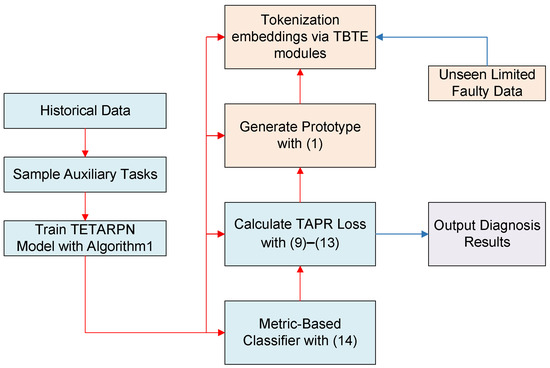
Figure 2.
TETARPN-based FSFD flowchart.
In the training phase, the proposed TETARPN framework is trained on the episodically sampled tasks from the training dataset , which includes known fault categories. As detailed in Algorithm 1, each training episode consists of a support set and a query set sampled from a subset of classes. During each episode, the model first extracts Transformer embeddings for both support and query samples, and then constructs class-wise prototypes using the support embeddings. A Task-Adaptive Prototype Regularization strategy is subsequently applied to jointly optimize classification performance and embedding space structure. The episodic optimization process encourages the model to generalize well to novel diagnostic tasks by learning a transferable embedding space and a robust metric-based decision boundary. After sufficient training episodes, the model parameters are optimized to .
| Algorithm 1 Learning Algorithm for TETARPN |
|
In the diagnosis (inference and deployment) phase, the trained TETARPN model is used to perform fault diagnosis on new, unseen tasks sampled from , containing previously unobserved fault types. In practical deployment, a few labeled instances from the new task are leveraged solely to define class prototypes in the embedding space. These instances are passed through the frozen Transformer encoder to extract their embeddings, which are then averaged to obtain task-specific prototypes . For any incoming data sample , its embedding is computed and compared against the prototypes to determine its class, enabling efficient, real-time diagnosis based on the learned metric:
where denotes the squared Euclidean distance.
Through this procedure, the proposed TETARPN method enables rapid adaptation to new diagnostic conditions with minimal labeled data. By integrating TBTE and TAPR, it achieves better FSFD performance across diverse and challenging working scenarios.
4. Experiments
4.1. Data Description
To evaluate the effectiveness of the proposed TETARPN method, we utilize a rolling bearing benchmark dataset provided by the Bearing Data Center of Case Western Reserve University (CWRU) [40], which has become a standard reference in the field of intelligent fault diagnosis. The CWRU dataset is available at https://engineering.case.edu/bearingdatacenter/download-data-file (accessed on 23 September 2025), which comprises vibration signals collected from the drive end of an induction motor using an accelerometer, with a uniform sampling rate of 12 kHz. The visualization of the vibration signal under ten categories is shown in Figure 3. Each dataset contains ten classes with a total of 4000 samples. The motor operates under four distinct load conditions, which correspond to rotational speeds of 1797, 1772, 1750, and 1730 revolutions per minute (rpm). For ease of reference, these operating conditions are categorized into subsets A, B, C, and D, respectively. Each subset includes one healthy condition and three typical fault types: inner race fault (IF), outer race fault (OF), and ball fault (BF). Moreover, each fault type is further divided into three damage severities—0.007, 0.014, and 0.021 inches—resulting in nine faulty categories and one normal condition per subset. Table 1 and Table 2 show our dataset settings under different loads.
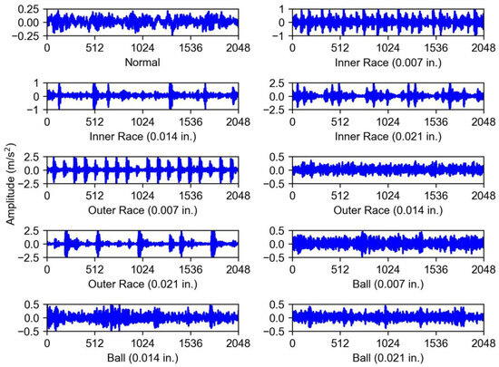
Figure 3.
The visualization of the vibration signal under ten categories from the CWRU Dataset [40].

Table 1.
Different categories of bearing faults selected from the CWRU dataset [40].
Table 2.
Task segmentation under four load conditions of the CWRU dataset.
To simulate a few-shot learning scenario, we follow an episodic training paradigm. Specifically, six of the ten categories (Classes 2–7) are designated as the training domain (), while the remaining four categories are reserved for testing (). For training, 1000 episodes are randomly generated. Each episode includes M fault categories randomly selected from , with K instances per category. For instance, under a 3-way 5-shot setting, three fault types are chosen and five samples from each are used, forming a support set of 15 samples for each episode. During the evaluation phase, 100 test episodes are sampled from following the same M-way K-shot setting to assess the average diagnostic accuracy.
4.2. Implementation Details and Evaluation Index
To evaluate the fault diagnosis performance of the proposed method, we conduct diagnostic performance tests on the CWRU bearing dataset and perform comparisons with other representative meta-learning approaches. In our Transformer-based Temporal Encoder Module, CWRU correspondences constitute a univariate time series. Given the extended sequence length of CWRU data required to capture fault characteristics, we configure l = 10,000 with segmentation granularity = 100. It is worth noting that the parameter is determined according to the specific experimental conditions. Its value is set to 30 for a 3-way setup and 40 for a 4-way setup. In our Task-Adaptive Prototype Regularization Module, the constant is set to 0.01, and and are both set to 0.5.
In our implementation, one iteration is equivalent to an epoch over the 1000 generated episodes, with training conducted for 50 iterations in total; the Adam optimizer is used with an initial learning rate of , decayed by a factor of after each iteration, while wall-clock time is not reported as it depends on hardware rather than the algorithmic setting. It is important to highlight that this study primarily investigates a novel FSFD method, utilizing bearing faults as the case study. This method is versatile and can be adapted for deployment across various hardware devices equipped with GPU computing units. All experiments were performed on a laptop featuring a GeForce RTX 3060 GPU (manufactured by ASUS Computer Co., Ltd., Taipei, Taiwan), utilizing PyTorch version 2.0.0. Theoretically, the proposed algorithm can be implemented on devices with comparable or even superior performance capabilities. To avoid randomness introduced by a single experiment, each setting was replicated five times. The overall FSFD performance of the proposed method was evaluated using the mean diagnostic accuracy and its confidence interval.
4.3. Result and Analysis
To demonstrate the superiority of the proposed TETARPN method, we conducted comparative experiments with several state-of-the-art meta-learning methods, including PN [25], PN-CL [27], PN-CTL [28], MatchingNet [26], RelationNet [41], and MAML [20]. Among them, PN employs the TBTE module to extract embedding features and compute prototypes, combining Euclidean distance and cross-entropy loss to build a metric-based FSFD model. PN-CL and PN-CTL are both derivative models of PN. What they have in common is that they both adopt a TBTE module similar to PN for embedding feature learning, but they differ in their optimization objectives: PN-CL integrates center loss with cross-entropy loss, while PN-CTL replaces cross-entropy loss with center triplet loss to further enhance the FSFD model. In addition, MatchingNet leverages an attention-based mechanism to map a small labeled support set to query samples for prediction. RelationNet introduces a learnable deep distance metric by constructing a relation module to measure the similarity between support and query samples. MAML, on the other hand, is a gradient-based approach that aims to learn an initialization of model parameters, enabling fast adaptation to new tasks with only a few gradient updates.
As shown in Table 3, the proposed TETARPN method consistently achieves higher accuracy than all compared meta-learning approaches on Dataset C. In the 3-way tasks, TETARPN obtains 90.93% and 93.10% under the 3-shot and 5-shot settings, respectively. These results are consistently above those of PN, PN-CL, and PN-CTL by margins ranging from 0.3% to over 3%, and also surpass the optimization-based (MAML) and relation/metric-based (RelationNet and MatchingNet) baselines. This indicates that TETARPN is able to form more discriminative prototypes even when the number of support samples is limited. In the more challenging 4-way tasks, TETARPN continues to demonstrate clear advantages, reaching 86.72% in the 3-shot case and 90.13% in the 5-shot case. Compared with the other methods, the improvements are generally within the range of 0.3–3.5%, showing that our method remains stable and effective even as task complexity increases. Notably, the margins become more pronounced in the 5-shot scenarios, which suggests that TETARPN is particularly adept at leveraging additional labeled samples to strengthen prototype representations and enhance generalization. Overall, these consistent gains across different baselines and setups confirm the robustness of the proposed framework. They further demonstrate that the task-adaptive design of TETARPN not only improves accuracy but also ensures strong adaptability to varying task complexities in few-shot fault diagnosis.
Table 3.
Few-shot diagnostic accuracy (%) with different meta-learning methods on Dataset C of CWRU under different setups.
To elaborate on the diagnostic accuracies of different methods, the confusion matrices are drawn in Figure 4. From the results, it can be seen that the proposed method achieves better discrimination between different categories and is not easily affected by other categories. At the same time, it is slightly better than other metric or meta variants in diagnostic accuracy.
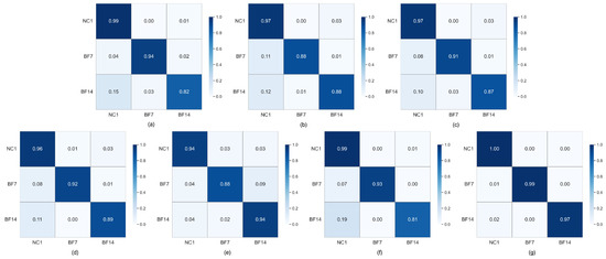
Figure 4.
Confusion matrix of different meta-learning methods on Dataset C under the 3-way 5-shot setting. (a) PN. (b) PN-CL. (c) PN-CTL. (d) MAML. (e) RelationNet. (f) MatchingNet. (g) TETARPN.
As demonstrated in Table 4, TETARPN consistently attains the highest F1-scores across all evaluated settings, including 3-way 3-shot, 3-way 5-shot, 4-way 3-shot, and 4-way 5-shot configurations. This superior performance highlights TETARPN’s effectiveness in few-shot diagnostic learning, outperforming conventional meta-learning approaches such as PN, PN-CL, MAML, and RelationNet. The bold formatting emphasizes the proposed method’s results for clarity.
Table 4.
F1-score (%) of different meta-learning methods on Dataset C under various experimental settings.
Furthermore, we conducted ablation experiments on TETARPN to test the impact of the TBTE and TAPR. As shown in Table 5, the method integrating the two modules has better FSFD performance. It can not only better deal with the temporal dependency problem of industrial data, but also has better adaptability when samples are scarce. This ablation study confirms that both the advanced temporal feature extraction capability of the TBTE and the adaptive regularization from the TAPR are critical and complementary components, and their synergistic combination is key to the model’s enhanced performance.
Table 5.
Few-shot diagnostic accuracy (%) of TETARPN with different components on Dataset C under different settings.
In addition to conducting comparative experiments on Dataset C with different methods, we also evaluated the effectiveness of the proposed method over various datasets under different loads. The experimental results are illustrated in Table 6. Clearly, TETARPN performs well in diagnosis tasks under various operating conditions, indicating that different operating loads do not excessively affect the diagnostic performance of our proposed method. As shown in Table 7, the proposed method consistently achieves high accuracy across all cross-scenario setups, including both 3-way and 4-way tasks. Accuracy generally improves with the number of shots, as 5-shot results are higher than 3-shot results in all cases. Among the three transfer scenarios, Dataset C to D achieves the highest accuracy, Dataset A to D the lowest, and Dataset B to D is intermediate, reflecting varying cross-domain adaptation difficulty. Notably, the smaller performance gains in the A to D scenario highlight cases where transferring to a domain with larger differences in operating conditions poses greater challenges. Overall, the method maintains stable performance even in the more challenging 4-way 3-shot tasks.
Table 6.
Few-shot diagnostic accuracy (%) of the proposed method on different datasets.
Table 7.
Few-shot diagnostic accuracy (%) of the proposed method on different datasets under cross-scenario setups.
Moreover, we visualize the FSFD performance of the proposed method under different meta-learning settings. As shown in Figure 5, our method has high accuracy and small performance fluctuation in different scenarios. However, although TETARPN achieves high overall accuracy, minor confusion between certain classes can be observed. For example, in Figure 5d, there are slight confusions between the NC1 and BF21 classes. This suggests that the vibration signals for these conditions may share some underlying characteristics, making them harder to separate, especially in a low-data regime. Such misclassifications likely stem from the inherent ambiguity and signal similarity between different machine states.
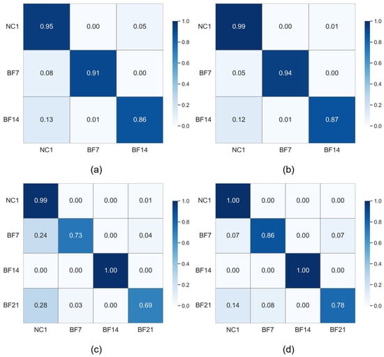
Figure 5.
Confusion matrix of features learned by TETARPN under different settings on dataset C. (a) 3-way 3-shot. (b) 3-way 5-shot. (c) 4-way 3-shot. (d) 4-way 5-shot.
Additionally, the hyperparameter selection experiments are conducted, and the corresponding results are recorded in Figure 6 and Table 8. From the results, it can be observed that the proposed method can effectively adapt to different parameter settings and perform stably. The best diagnostic accuracy is achieved at loss weights and tokenization granularity configuration , respectively. The optimal learning rate and decay factor have been determined to be 0.001 and 0.4, respectively, based on the performance of the diagnostic evaluation.
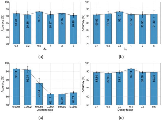
Figure 6.
Few-shot diagnostic accuracy (%) of TETARPN with different hyperparameters on Dataset C under the 3-way 5-shot setting. (a) . (b) . (c) Learning rate. (d) Decay factor.
Table 8.
Few-shot diagnostic accuracy (%) of TETARPN with different subsequence granularity on Dataset C Under the 3-way 5-shot settings.
5. Conclusions
In this work, we develop a new meta-learning approach termed TETARPN to tackle the FSFD challenges in complex industrial environments. The proposed TETARPN method includes two well-designed modules, named TBTE and TAPR. It not only improves the quality of learned representations through self-attention mechanisms that capture long-range temporal dependencies, but also adaptively refines the feature space in response to task-specific difficulty, thereby achieving a more balanced trade-off between adaptability and generalization. Comprehensive experiments demonstrate that TETARPN consistently outperforms baselines, including PN and its variants, across diverse operating conditions and varying levels of data scarcity, underscoring its potential for practical deployment in real-world diagnostic scenarios. Although the proposed framework achieves competitive performance, we identify three key directions for future work. First, its scalability to more complex multivariate scenarios where data is collected from multiple sensors requires further investigation to effectively model cross-channel dependencies. Second, future work could explore extending this framework to address the more challenging cross-domain fault diagnosis issue, such as cross-machine scenarios, to improve the model’s robustness and domain generalization capability. Third, to address the misclassifications stemming from the high similarity between certain fault signals, future research can focus on developing more discriminative feature learning methods that are robust to signal ambiguities, especially in low-data regimes.
Author Contributions
Conceptualization, M.X.; methodology, H.P.; software, S.S.; validation, M.X., H.P., and S.W.; formal analysis, H.P.; investigation, S.W.; resources, S.S.; data curation, S.S.; writing—original draft preparation, S.S.; writing—review and editing, M.X.; visualization, S.S.; supervision, M.X.; project administration, M.X.; funding acquisition, M.X. All authors have read and agreed to the published version of the manuscript.
Funding
This work is supported by the Science and Technology Project of State Grid Shandong Electric Power Company, named Research on brain-like sensing technology of multi-sensor module for substation intelligent inspection device (No. 52060122000P).
Data Availability Statement
The original data presented in the study are openly available at https://engineering.case.edu/bearingdatacenter/download-data-file (accessed on 23 September 2025).
Conflicts of Interest
Author Mingkai Xu, Huichao Pan and Siyuan Wang were employed by the company State Grid Shandong Electric Power Company, Jinan Power Supply Company. The remaining authors declare that the research was conducted in the absence of any commercial or financial relationships that could be construed as a potential conflict of interest.
References
- Li, J.; Wang, F. Transformer Fault Diagnosis Using Hybrid Feature Selection and Improved Black-Winged Kite Optimized SVM. Electronics 2025, 14, 3160. [Google Scholar] [CrossRef]
- Al Lahham, E.; Kanaan, L.; Murad, Z.; Khalid, H.M.; Hussain, G.A.; Muyeen, S. Online condition monitoring and fault diagnosis in wind turbines: A comprehensive review on structure, failures, health monitoring techniques, and signal processing methods. Green Technol. Sustain. 2025, 3, 100153. [Google Scholar] [CrossRef]
- Veigas, K.L.; Chinnici, A.; De Chiara, D.; Chinnici, M. Towards Energy Efficiency of HPC Data Centers: A Data-Driven Analytical Visualization Dashboard Prototype Approach. Electronics 2025, 14, 3170. [Google Scholar] [CrossRef]
- Danso, A.A.; Büker, U. Automated Generation of Test Scenarios for Autonomous Driving Using LLMs. Electronics 2025, 14, 3177. [Google Scholar] [CrossRef]
- Zhao, M.; Zhong, S.; Fu, X.; Tang, B.; Pecht, M. Deep residual shrinkage networks for fault diagnosis. IEEE Trans. Ind. Inform. 2019, 16, 4681–4690. [Google Scholar] [CrossRef]
- Zuo, F.; Liu, J.; Ren, Y.; Wang, L.; Wen, Z. A Reliable Bolt Key-Points Detection Method in Industrial Magnetic Separator Systems. IEEE Trans. Instrum. Meas. 2025, 74, 5015710. [Google Scholar] [CrossRef]
- Mukherjee, C. Machine Learning Approaches for Fault Detection in Pipeline Flowlines. 2025. Available online: https://www.researchgate.net/profile/Chandrani-Mukherjee-2/publication/395354454_Machine_Learning_Approaches_for_Fault_Detection_in_Pipeline_Flowlines/links/68bfa0596f87c42f3b91064f/Machine-Learning-Approaches-for-Fault-Detection-in-Pipeline-Flowlines.pdf (accessed on 26 September 2025).
- Cheng, Y.; Yan, J.; Zhang, F.; Li, M.; Zhou, N.; Shi, C.; Jin, B.; Zhang, W. Surrogate modeling of pantograph-catenary system interactions. Mech. Syst. Signal Process. 2025, 224, 112134. [Google Scholar] [CrossRef]
- Chen, C.; Li, X.; Shi, J. Hierarchical gray wolf optimizer-tuned flexible residual neural network with parallel attention module for bearing fault diagnosis. IEEE Sens. J. 2024, 24, 19626–19635. [Google Scholar] [CrossRef]
- Chen, C.; Wang, Z.; Shi, J.; Yue, D.; Shi, G.; Wang, C. Noise-Resilient Bearing Fault Diagnosis via Hybrid Attention-Based Multi-Scale ScConv and Quaternion Transformer. IEEE Trans. Instrum. Meas. 2025, 74, 3552118. [Google Scholar]
- Zhao, J.; Wang, W.; Huang, J.; Ma, X. A comprehensive review of deep learning-based fault diagnosis approaches for rolling bearings: Advancements and challenges. AIP Adv. 2025, 15, 020702. [Google Scholar] [CrossRef]
- Łuczak, D. Data-driven machine Fault Diagnosis of Multisensor vibration data using synchrosqueezed transform and time-frequency image recognition with convolutional neural network. Electronics 2024, 13, 2411. [Google Scholar] [CrossRef]
- Calabrese, F.; Regattieri, A.; Bortolini, M.; Galizia, F.G. Data-driven fault detection and diagnosis: Challenges and opportunities in real-world scenarios. Appl. Sci. 2022, 12, 9212. [Google Scholar] [CrossRef]
- An, Y.; Zhang, K.; Liu, Q.; Chai, Y.; Huang, X. Deep transfer learning network for fault diagnosis under variable working conditions. In Proceedings of the 2021 CAA Symposium on Fault Detection, Supervision, and Safety for Technical Processes (SAFEPROCESS), Chengdu, China, 17–18 December 2021; pp. 1–6. [Google Scholar]
- Wu, J.; Zhao, Z.; Sun, C.; Yan, R.; Chen, X. Few-shot transfer learning for intelligent fault diagnosis of machine. Measurement 2020, 166, 108202. [Google Scholar] [CrossRef]
- Wang, J.; Lan, C.; Liu, C.; Ouyang, Y.; Qin, T.; Lu, W.; Chen, Y.; Zeng, W.; Yu, P.S. Generalizing to unseen domains: A survey on domain generalization. IEEE Trans. Knowl. Data Eng. 2022, 35, 8052–8072. [Google Scholar] [CrossRef]
- Li, H.; Pan, S.J.; Wang, S.; Kot, A.C. Domain generalization with adversarial feature learning. In Proceedings of the IEEE Conference on Computer Vision and Pattern Recognition (CVPR), Salt Lake City, UT, USA, 18–23 June 2018; pp. 5400–5409. [Google Scholar]
- Jing, L.; Tian, Y. Self-supervised visual feature learning with deep neural networks: A survey. IEEE Trans. Pattern Anal. Mach. Intell. 2020, 43, 4037–4058. [Google Scholar] [CrossRef] [PubMed]
- Fu, Y.; Xue, F. Mad: Self-supervised masked anomaly detection task for multivariate time series. In Proceedings of the 2022 International Joint Conference on Neural Networks (IJCNN), Padua, Italy, 18–23 July 2022; pp. 1–8. [Google Scholar]
- Finn, C.; Abbeel, P.; Levine, S. Model-agnostic meta-learning for fast adaptation of deep networks. In Proceedings of the International Conference on Machine Learning (ICML), Sydney, Australia, 6–11 August 2017; pp. 1126–1135. [Google Scholar]
- Li, K.; Wang, L.; Gao, X.; Zhang, L. Transformer-enhanced meta-learning for few-shot fault diagnosis of electric submersible pump. Expert Syst. Appl. 2025, 284, 127851. [Google Scholar] [CrossRef]
- Balaji, Y.; Sankaranarayanan, S.; Chellappa, R. Metareg: Towards domain generalization using meta-regularization. Adv. Neural Inf. Process. Syst. NeurIPS 2018, 31. Available online: https://proceedings.neurips.cc/paper_files/paper/2018/file/647bba344396e7c8170902bcf2e15551-Paper.pdf (accessed on 1 September 2025).
- Yue, F.; Wang, Y. Cross-domain fault diagnosis via meta-learning-based domain generalization. In Proceedings of the 2022 IEEE 18th International Conference on Automation Science and Engineering (CASE), Mexico City, Mexico, 20–24 August 2022; pp. 1826–1832. [Google Scholar]
- Hospedales, T.; Antoniou, A.; Micaelli, P.; Storkey, A. Meta-learning in neural networks: A survey. IEEE Trans. Pattern Anal. Mach. Intell. 2021, 44, 5149–5169. [Google Scholar] [CrossRef]
- Snell, J.; Swersky, K.; Zemel, R. Prototypical networks for few-shot learning. Adv. Neural Inf. Process. Syst. NeurIPS 2017, 30, 4077–4087. [Google Scholar]
- Vinyals, O.; Blundell, C.; Lillicrap, T.; Wierstra, D. Matching networks for one shot learning. Adv. Neural Inf. Process. Syst. NeurIPS 2016, 29. [Google Scholar] [CrossRef]
- Yu, T.; Guo, H.; Zhu, Y. Center Loss Guided Prototypical Networks for Unbalance Few-Shot Industrial Fault Diagnosis. Mob. Inf. Syst. 2022, 2022, 3144950. [Google Scholar] [CrossRef]
- Qiu, Y.; Liu, H.; Liu, J.; Shi, B. Center-triplet loss for railway defective fastener detection. IEEE Sens. J. 2023, 24, 3180–3190. [Google Scholar] [CrossRef]
- Tseng, H.Y.; Lee, H.Y.; Huang, J.B.; Yang, M.H. Cross-domain few-shot classification via learned feature-wise transformation. arXiv 2020, arXiv:2001.08735. [Google Scholar]
- Liu, J.; Song, L.; Qin, Y. Prototype rectification for few-shot learning. In Proceedings of the European Conference on Computer Vision (ECCV), Glasgow, UK, 23–28 August 2020; Springer: Berlin/Heidelberg, Germany, 2020; pp. 741–756. [Google Scholar]
- Sehri, M.; Hua, Z.; Boldt, F.d.A.; Dumond, P. Selective Embedding for Deep Learning. arXiv 2025, arXiv:2507.13399. [Google Scholar] [CrossRef]
- Zhang, Y.; Tang, Y.; Liu, Y.; Liang, Z. Fault diagnosis of transformer using artificial intelligence: A review. Front. Energy Res. 2022, 10, 1006474. [Google Scholar] [CrossRef]
- Saeed, A.; Khan, M.A.; Akram, U.; Obidallah, W.J.; Jawed, S.; Ahmad, A. Deep learning based approaches for intelligent industrial machinery health management and fault diagnosis in resource-constrained environments. Sci. Rep. 2025, 15, 1114. [Google Scholar] [CrossRef]
- Li, K.; Shang, C.; Ye, H. Reweighted Regularized Prototypical Network for Few-Shot Fault Diagnosis. IEEE Trans. Neural Netw. Learn. Syst. 2022, 35, 6206–6217. [Google Scholar] [CrossRef]
- Wang, S.; Wang, D.; Kong, D.; Wang, J.; Li, W.; Zhou, S. Few-shot rolling bearing fault diagnosis with metric-based meta learning. Sensors 2020, 20, 6437. [Google Scholar] [CrossRef]
- Qin, Y.; Wen, Q.; Wang, L.; Mao, Y. Adaptive generic prototype network with geodesic distance for cross-domain few-shot fault diagnosis. Knowl.-Based Syst. 2024, 306, 112726. [Google Scholar] [CrossRef]
- Jiang, C.; Chen, H.; Xu, Q.; Wang, X. Few-shot fault diagnosis of rotating machinery with two-branch prototypical networks. J. Intell. Manuf. 2023, 34, 1667–1681. [Google Scholar] [CrossRef]
- Wang, L.; Zhang, H.; Liu, J.; Zuo, F. Knowledge Transfer and Reinforcement Based on Biunbiased Neural Network: A Novel Solution for Open-Set Fault Transfer Diagnosis. IEEE Trans. Neural Netw. Learn. Syst. 2025, 36, 15794–15806. [Google Scholar] [CrossRef]
- Vaswani, A.; Shazeer, N.; Parmar, N.; Uszkoreit, J.; Jones, L.; Gomez, A.N.; Kaiser, Ł.; Polosukhin, I. Attention is all you need. Adv. Neural Inf. Process. Syst. NeurIPS 2017, 30. Available online: https://proceedings.neurips.cc/paper_files/paper/2017/file/3f5ee243547dee91fbd053c1c4a845aa-Paper.pdf (accessed on 1 September 2025).
- Loparo, K. Case Western Reserve University Bearing Data Center; Bearings Vibration Data Sets; Case Western Reserve University: Cleveland, OH, USA, 2013; pp. 22–28. [Google Scholar]
- Sung, F.; Yang, Y.; Zhang, L.; Xiang, T.; Torr, P.H.; Hospedales, T.M. Learning to compare: Relation network for few-shot learning. In Proceedings of the IEEE Conference on Computer Vision and Pattern Recognition, Salt Lake City, UT, USA, 18–23 June 2018; pp. 1199–1208. [Google Scholar]
Disclaimer/Publisher’s Note: The statements, opinions and data contained in all publications are solely those of the individual author(s) and contributor(s) and not of MDPI and/or the editor(s). MDPI and/or the editor(s) disclaim responsibility for any injury to people or property resulting from any ideas, methods, instructions or products referred to in the content. |
© 2025 by the authors. Licensee MDPI, Basel, Switzerland. This article is an open access article distributed under the terms and conditions of the Creative Commons Attribution (CC BY) license (https://creativecommons.org/licenses/by/4.0/).