Article

Integrated Soft-Sensor Model for Wastewater Treatment Process with Collaborative Calibration Strategy

1
Department of Aerospace Science and Technology, Space Engineering University, Beijing 101416, China
2
College of Information Science and Technology, Beijing University of Technology, Beijing 100124, China
*
Author to whom correspondence should be addressed.
Electronics 2025, 14(22), 4506; https://doi.org/10.3390/electronics14224506
Submission received: 4 October 2025 / Revised: 14 November 2025 / Accepted: 17 November 2025 / Published: 18 November 2025
(This article belongs to the Section Systems & Control Engineering)

Abstract

The soft-sensor model (SSM) has been widely used for monitoring water quality, operational state, and performance evaluation in wastewater treatment process (WWTP). However, due to serious dynamics in WWTP under different working conditions, SSM faces a challenge to maintain excellent performance. To address this issue, an integrated soft-sensor model (ISSM) is introduced for WWTP based on a collaborative calibration strategy in this study. Different from the previous studies, the SSM is equipped with the given model structure with respect to certain input variables. The proposed ISSM has the capability of updating its structure online to adapt to the changes in input variables with a structural collaborative calibration strategy. The parameters of ISSM, associated with feature extraction of input variables and feature representation of its input–output, are calibrated simultaneously with a parametric collaborative calibration strategy. As a result, this model can improve its adaptability to the dynamics of WWTP and further maintain the accuracy of real-time monitoring. Finally, the ISSM is used to monitor the total nitrogen removal in WWTP. Its RMSE on the test set is lower than that of most comparison algorithms, with a streamlined network architecture enabling monitoring, which validates its effectiveness and advanced nature.

Graphical Abstract

1. Introduction

Over the past few years, driven by both advances in environmental protection technology and heightened awareness of the hazards of eutrophication, the requirements and standards for wastewater treatment processes (WWTPs) have become increasingly stringent [1,2,3]. It is essential for WWTPs to monitor the key or primary process indicators associated with its instrumentation, control, and automation [4,5]. As an alternative monitoring method, the soft-sensor model (SSM) represents an efficient and cost-effective technical solution capable of directly extracting and modeling relevant process information from routine process and laboratory data [6,7,8]. It finds widespread application in the field of fault detection and diagnosis, online prediction, and so on [9,10]. The essence of the SSM lies in establishing a mathematical model that exploits available input and associated output data to describe their relationships, which in turn reflects core variables that are difficult to measure [11]. Therefore, the selection of input variables selection and model design of the SSM are crucial to maintain its acceptable performance.
By reducing the dimensionality of input variables, variable selection can effectively lower costs, which improves the feasibility of implementing practical applications. It also avoids the problem of overfitting and increasing calculation time caused by too many parameters [12]. Some efficient methods like principal component analysis (PCA) [13], partial least squares (PLS) [14], and a series of PLS-based methods [15,16,17], for variable selection have already been developed. They exploit linear manifold techniques to achieve dimensionality reduction by mapping observations onto a low-dimensional subspace. However, this type of technique cannot accomplish the variable selection accurately due to the nonlinearity of WWTP. To capture the nonlinear relationships between variables, kernel-based approaches have been the subject of extensive research, such as kernel PCA (KPCA) and kernel PLS (KPLS) [18]. This process is first achieved by transforming the original data into a high-dimensional feature space through a nonlinear mapping. Based on this, the high-dimensional feature space is analyzed using PCA/PLS methods [19]. Specifically, Huang et al. proposed a method for extracting independent and related variables by using KPCA and support vector data description [20]. Deng et al. developed an improved KPCA to obtain the feature variables based on deep principal component analysis [21]. Si et al. presented an improved KPLS, which provided a reasonable decomposition of process information [22]. It had a high efficiency in observing the correlation between variables. However, methods based on KPCA and KPLS have certain limitations, which only exploit the partial correlation information of the selected latent variables. To address this problem, Wang and Jiao designed a kernel least squares (KLS) model to exploit the entire correlation of selected latent variables and determine their number [23]. Furthermore, by considering that the traditional kernel-based methods ignore the regression relationships between variables, Wei and Song introduced a supervised kernel-learning model for process monitoring online [24], which is suitable for variable selection by sharpening the authentic relationship between variables.
Model design is another core in the development of SSM, which prepares the model structure and its parameters to map the relationship between inputs and outputs. Although there is no consistent approach to accomplish this task so far, several techniques have been studied to provide a reliable model for SSM. For instance, Cheng et al. proposed a kernel machine learning model to describe nonlinear problems in multivariate ICs data [25]. The exploratory analysis through data visualization revealed the temporal behavior and statistical characteristics of multivariate IC time series. Abouzari et al. introduced twelve linear and nonlinear regression models to estimate the chemical oxygen demand (COD) level [26]. These models serve as efficient alternatives for estimating chemical oxygen demand (COD), with accuracy that overcomes the time-consuming and labor-intensive bottlenecks of traditional laboratory analysis. Although statistical models or regression models have the advantages of simple calculation and strong interpretability, they are not suitable for covering the complexity and nonlinearity of WWTP [27,28]. Then, some researchers tried to model WWTP with the collected data using support vector machine (SVM) [29,30], neural networks (NNs) [31,32,33]. They can capture the dynamic nonlinear relationships of variables in the WWTP well. Tan et al. proposed SVM to forecast the discharge nitrate concentration with an adaptive neuro-fuzzy reasoning system model [34]. Nourani et al. designed an LSSVM method to realize the continuous forecasting of effluent COD in an anaerobic wastewater treatment system [35]. The calculating procedure can be sped up, and the calculation performance can be improved significantly in the above method, which alleviates the fact that the calculating process is complicated and difficult to execute for the size of the training data [36]. However, these methods cannot process data online, and the selection of the kernel function requires subjective participation [37]. Compared with these methods, some intelligent methods have stronger learning ability and autonomy, and can realize the learning and training of data only by data supervision. As intelligent methods, fuzzy reasoning systems and artificial neural networks have been widely used in WWTP [38,39], but both have their strengths and weaknesses. In this case, the fuzzy neural network (FNN) was proposed, which can combine the learning ability of a neural network with the interpretability of a fuzzy system based on rules, and has considerable accuracy and convergence speed [40]. Unfortunately, in most FNNs, only the learning stages of parameters are determined by learning algorithms, and their structures are artificially fixed in advance. Improper selection of fuzzy rules may lead to problems in accuracy or real-time performance. To obtain a tight network structure of FNNs, a dynamic fuzzy neural network (DFNN) was proposed in [41] to determine the number of fuzzy rules. Then, a generalized dynamic fuzzy neural network (GDFNN), an enhanced version of DFNN, was developed in [42]. However, both DFNN and GDFNN are confined to offline learning modes and lack online adaptive capabilities. Additionally, the existing publications associated with variable selection and model design of SSM still have the following problems:
(1) Although the proposed SSM has the capability of describing the input–output relationship between variables with available data, it performs the variable selection and model design asynchronously or modifies the model with given variables directly. This SSM is hard to adapt to the change in working conditions, where the categories of input variables related to primary variables also change.
(2) The carrier of SSM, such as DNN, DFNN, GDFNN, has realized that the structure of these models can self-organize or be adjusted following the underlying regularity derived from given data. The standards, importance, and sensitivity of neuron or fuzzy rules that direct the update of structure are usually implemented with evaluation of input classification, structural complexity, and output performance, etc., but ignore the change in inputs, which includes their dimension and attribution.
(3) The parameter learning of SSM generally involves least squares, gradient descent, evolutionary algorithms, etc., which are merely conducted in continuous dimensional space. Once the working conditions change, the dimension of parameters should be updated over time to match the dimension of inputs. Without any prior knowledge, it brings an obstacle for SSM to hold a stable performance during the switch of working conditions.
Inspired by the above challenges, this study proposes an integrated soft-sensor model (ISSM) for WWTP based on a collaborative calibration strategy. The proposed model updates its structure online with a structure collaborative calibration strategy and its parameters with a collaborative calibration strategy. As a result, this model can adapt to the change in input variables arbitrarily, following the dynamics of working conditions. The contributions of this study are as follows:
(1) The proposed ISSM is built by inserting a feature extraction layer with sets of gated units into a traditional self-organizing fuzzy neural network. This model simultaneously performs variable selection and model design synchronously according to the state of working conditions.
(2) Compared to the existing SSMs employing a self-organized structure, the proposed ISSM dynamically adjusts its architecture through a structural collaborative calibration strategy. This strategy dynamically modulates the number of gating units and neurons, simultaneously balancing output performance, structural complexity, and input space. They will promote ISSM to find the optimal structure online.
(3) To maintain the stable performance of ISSM, a parametric collaborative calibration strategy is designed. This strategy can coordinate the parameters of feature extraction and feature representation to suppress the abrupt change in parametric space by a re-weighted regularized conjugate gradient method.
The structure of this study is as follows: Section 2 reviews the fundamental principles of soft sensors for WWTPs. Section 3 describes in detail the proposed ISSM, which includes an improved gated unit, the self-organizing mechanism of FNN, as well as the collaborative calibration strategy. Section 4 presents the experimental results of ISSM, which highlight its advantages in applicability and accuracy over existing methods. Section 5 concludes this study.

2. Preliminaries

In recent years, soft sensors have been regarded as the mainstream method for the practical monitoring of WWTP [9,43]. Deep neural networks learn from historical data, encoding complex patterns within the network parameters to accomplish prediction tasks. However, the efficiency of this process is often constrained by the complexity of the model hyperparameter optimization procedure [44]. Soft sensors can achieve great monitoring performance without complex mechanism knowledge of WWTP, and only use observational data. Its inputs originate from auxiliary variables that are easily measurable, specifically manifested as process signals, measurement data, and expert knowledge. The model’s output targets are those dominant variables that are difficult to measure online [45]. The mapping relationship between input and output is derived through empirical modeling, which is encoded with the available data. The role of SSM is to construct a dynamic model that can provide real-time estimates of output variables for new input data. Therefore, the core task of SSM in addressing supervised learning problems is essentially to perform regression or classification.
However, it is a common practice to observe degradation of soft sensors in continuous data streams in practice. The change in process and instrument characteristics or operating conditions is typically the cause of this performance degradation. The reasons primarily stem from two aspects: one is the variation in operating conditions, such as influent water quality, temperature, and flow rate; the other is equipment and management factors, such as changes in instrument calibration and operational procedures. The above changes can be described as the statistical characteristics of the target variable frequently altered by the input variables, which is called concept drift in machine learning. The phenomenon will degrade the performance of soft sensors. A series of algorithms have emerged to preset a model, such as a diversity pool, or to preprocess the learning pattern, including batch learning and just-in-time-learning algorithms. They are generally available for the gradual drift during long-term WWTP. They still consume effort of preliminary decision-making, which makes it hard to solve the sudden drift with the change in operating point or reaction stage.

3. Self-Organizing Fuzzy Neural Network with Feature Extraction Layer

In this section, ISSM and its mechanism are described in detail. After that, the feature selection method and self-organizing strategy involved in the framework of the integrated soft-sensor (F-FNN) are described systematically. Then, the collaborative optimization process of this network is introduced.

3.1. Framework of Integrated Soft-Sensor

The proposed ISSM is constructed based on data-driven principles, which integrate variable selection and model design to achieve dynamic feature evaluation and expression in a changing environment. ISSM follows the same process as conventional data-driven soft sensors, with independent steps including data acquisition, preprocessing, model design, and maintenance. This process is essentially an iterative cycle requiring continuous optimization. The specific flow of ISSM is shown in Figure 1, and each step will be further described below.

3.1.1. Data Acquisition

The operational data for ISSM originates from an actual anaerobic anoxic oxic (A2/O) WWTP in operation. The process units of this wastewater treatment system comprise two anaerobic tanks, two anoxic tanks, and four aerobic zones. In this plant, online measuring instruments are set up in advance in the corresponding reaction tanks. These online instruments are deployed in each reaction tank of the A2/O process to measure a series of readily accessible parameters. The measured parameters include dissolved oxygen concentration (DO), ammonia nitrogen (NH4-N), nitrate nitrogen (NO3-N), oxidation–reduction potential (ORP), total suspended solids (TSSs), potential of hydrogen (PH), and temperature (T). To ensure data acquisition frequency, all devices operate in continuous measurement mode and store data in local memory. To achieve centralized management and distribution of data, uploaded data is received and integrated by an Open Process Control (OPC) server.

3.1.2. Data Preprocessing

This step aims to transform the data to ensure that the prediction model can process the data more efficiently. Figure 1 shows several necessary processing steps for processing data generated in the WWTP. The usual processing steps include missing data processing, outlier detection and replacement, selection of related variables, handling of drift data, and delay detection between particular variables. At this stage, many steps are handled manually, and a large proportion of data processing needs to be judged by the model developer. In the designed data preprocessing method, data cleaning and sample selection are carried out iteratively until the data is ready for training and evaluation of the actual model, after only one standardization and missing value processing. It is remarkable that, in this step, the feature selection process is integrated into the model design, which previously required substantial manual intervention. This integration enables the model to automatically evaluate and select features, thereby significantly reducing manual effort and enhancing the feasibility of the ISSM.

3.1.3. Model Design

In this study, a multi-input single-output F-FNN is introduced. A regular FNN consists of only four layers: the input layer, the RBF layer, the normalization layer, and the output layer. This network is equipped with an extra feature extraction layer compared to the regular FNN, which has the capability of dynamic feature extraction and expression with a change in inputs.
The specific description of F-FNN is as follows:
Input layer: There are m neurons in this layer, which represent the input variables of F-FNN. It consists of feature subsets as
X = x 1 , x 2 , , x i , , x m ,
where xi is ith neuron, i = 1, 2,…, m.
Feature extraction layer: The weight connection formed by this layer can approximate any function, so that the feature extraction part can accurately evaluate the input features. There are P neurons, which all contain tangent sigmoid functions. The output values of neurons in this layer are
U = σ ( X T W + b ) ,
u k = g ( w k 1 x 1 + w k 2 x 2 + + w k m x m + b k ) ,
where uk is the kth output value, U = [u1, u2,…, uk,… uN], k = 1, 2,…, N. W is the weights parameter matrix, W = [w1, w2,…, wk,…, wP], wk= [wk1, wk2,…, wkm], b is the bias between the kth neuron in the feature extraction layer and the input layer, b = [b1, b2,…, bk], σ(·) is an activation function, and g(·) is tangent sigmoid function.
Pooling layer: This layer receives the evaluated feature set and selects the most appropriate feature subset according to the adaptive threshold T as the input of the next layer. The number of neurons in this layer is equivalent to the number of feature subsets after selection, which is the floating value changed according to the threshold T selection. Assume the floating value to N. The output is represented as follows:
u i = u k ,
where ui is the output of the pooling layer, and its value is uk, i = 1, 2,…, N.
RBF layer: The functionality of this layer is implemented by Q radial basis function (RBF) neurons, each corresponding to a precondition of a fuzzy rule. The output values of these RBF neurons are given by
ϕ j = i = 1 N e ( ( u i c i j ) 2 / 2 σ i j 2 ) = e i = 1 N ( ( u i c i j ) 2 / 2 σ i j 2 ) ,
where e is the natural constant, ui is the input value, U = [u1, u2,…, ui,…, uN], σj and cj are the vectors of widths and centers of the jth RBF neuron, respectively, σj = [σ1j, σ2j,…, σNj], cj = [c1j, c2j,…, cNj], j = 1, 2,…, Q.
Normalized layer: There are Q neurons in this layer
v l = ϕ l j = 1 Q ϕ j = e i = 1 N ( ( u i c i j ) 2 / 2 σ i j 2 ) j = 1 Q e i = 1 N ( ( u i c i j ) 2 / 2 σ i j 2 ) ,
where vl is lth neurons output values, l = 1, 2,…, Q, v = [v1, v2,…, vl,…, vQ]T.
Output layer: The output layer has only one neuron, calculated as
g ^ = W v ,
W = w 1 , w 2 , , w Q ,
where W′ is a parameter matrix between the normalized and the output layer. The detailed calculation of the output value is
g ^ = W v = l = 1 Q w l e i = 1 N ( ( u i c i j ) 2 / 2 σ i j 2 ) j = 1 Q e i = 1 N ( ( u i c i j ) 2 / 2 σ i j 2 )

3.1.4. Model Maintenance

In order to avoid soft sensor performance degradation caused by data drift and other changes, compensation must be made by adjusting or redeveloping the model. Therefore, this model must be maintained regularly. This study presents a real-time model maintenance scheme. The label data provided by the experimental analysis provides the basis for the supervised modification of the model. The self-organizing mechanism carried by F-FNN will enable it to change the network structure in different data distributions, which makes the network obtain a stronger generalization ability. The core of this approach lies in online monitoring of input data streams and triggering multi-level model adaptive behavior based on quantitative assessments of feature distribution drift. Specifically, Martensitic Distance (MD) is calculated from real-time feature vectors to precisely detect shifts in data distribution. The threshold for the feature drift metric is established to guide model maintenance decisions. There are two cases of model modification and reconstruction in model maintenance. When the data distribution changes slowly, the network weight is adjusted periodically to maintain the reliability of the model. However, once the data distribution changes greatly, the feature selection part will first reflect the changes in the selected feature subset, and then the network will appropriately increase or decrease the neurons in the rule layer under the guidance of the self-organization mechanism.

3.2. Feature-Based Fuzzy Neural Network

The aforementioned study provides an overall description of the layer-by-layer structure of the F-FNN. However, during design, this network consists of two network structures with a coupling relationship, and the training of the entire network is conducted separately for each part. The front part of the network architecture resembles a multi-layer perceptron (MLP), while the subsequent structure can be regarded as a typical FNN. In the former approach, the input space is determined by training the network weights, evaluating and ranking feature sets that are guided by adaptive thresholds to select the optimal feature subset through an aggregation layer. In the latter, FNN is equipped with a self-organizing mechanism to follow the change in feature subset and automatically choose whether to add or subtract neurons.

3.2.1. Feature Extraction Method

In this study, the feature extraction method is used as an evaluation index to calculate the contribution rate of input features, which can obtain the sensitivity of the network output to small input disturbances by calculating the partial derivative of the network.
The disturbance of the inputs and outputs can be represented by its Jacobian matrix dy/dx = [ϑyx]m×n. The feature extraction part of this study can be regarded as an MLP with m inputs and one output, then the gradient vector of y relative to xi can be described as di = [d1,…, di,…, dm] with
d i = S i h = 1 P w ( 1 I i k 2 ) w ,
where Si is the derivative of the output node with respect to its input, Iik is the output of the kth hidden node for the tth input, the scalar w is the weight between the ith input node and the kth hidden node, and w′ is the weight between the output node and the kth hidden node.
By employing the sum of squared partial derivatives (SSDs) as a metric, the relative contribution of the ith input variable to a specific output can be calculated as follows:
S S D i = i = 1 T d i 2 ,
where T is the number of data. Different from algorithms requiring iteration, the SSD value directly reflects the impact of each input variable on the output.
The network uses a recursive feature elimination (RFE) approach for feature selection, pruning the input neurons with the least contribution in each iteration, and giving greater weight to the important input variables. Assume training is performed on dataset A, A = {(x(h), yd(h)); h = 1,…, H}. The following algorithmic feature elimination process is outlined.
To maintain the stability of the sum of inputs to hidden layer neurons, after identifying the input node xi to be removed, all its output connections must be eliminated, and the remaining input weights in its projection domain must be updated accordingly. That is, the following conditions are satisfied:
x i ( h ) X w i k x i ( h ) = x i ( h ) X r ( w i k + δ i k ) x i ( h ) ,
where i = 1,…, r − 1, r + 1,…, m, k = 1,…, P, and the quantities δik are the adjusting factors for the weights wik. This prevents the need to retrain the entire network. Further, it is simplified as
x i X r δ i k x i ( h ) = w r k x r ( h ) ,
The information measurement function is employed as the evaluation function of a heuristic search method, which is based on the minimum redundancy and maximum correlation criteria. Feature selection refers to finding a subset S from the feature set F to make it approximate the amount of information between category C and F, e.g., eFeS, where eF is the error of the classification model hF.
The heuristic sequence selection method assumes that each selection of a feature will increase the information content of the selected subset S, and its quantitative form is J (S) ≤ J(S, f). In this case, the J(S) computing problem is transformed into the problem of calculating J(f), which significantly lowers the computational complexity of the selection process and enhances the reliability of the mutual information estimation.
The information measurement function of candidate feature f in this study is
J ( f ) = I ( C ; f ) 1 | S | s S I ( s ; f ) ,
I ( C ; f ) = f F p ( C , f ) log 2 p ( C , f ) p ( C ) p ( f ) ,
I ( s ; f ) = s S f F p ( s , f ) log 2 p ( s , f ) p ( s ) p ( f ) ,
where p(s) and p(f) are the single-variable marginal, I(C; f) indicates the amount of information of candidate features, I(s; f) denotes the redundancy between f and subset S. When J(f) is greater than 0, the candidate features are added to the subset S. When J(f) is less than or equal to 0, the candidate features are eliminated.
The proposed feature extraction method is shown in Algorithm 1.
Algorithm 1: The variable selection method.
1: Input: Dataset: A = ( x ( k ) , y d ( k ) ) ; k = 1 , , m ;
2: Output: Optimal feature set X;
3: Set M ( A ) ← “Network trained with dataset A”
4: for k = m down to 1
5:  For each x i X , compute S S D i , Equation (11), and let x r = arg min x i X ( S S D i ) ;
6:  X X \ x r , “Remove variable x r that has the lowest S S D i ”;
7:  Set M ( A ) ← “Network updated by removing the x r input and adjusting the remaining weights according to Equation (12), and w i j ( n e w ) = w i j ( o l d ) + δ i j ”.
8:  Calculate the mutual information I ( X ; C ) of X and C;
9:  If I ( X ; C ) I 0 “Control the amount of feature selection by threshold I 0 ”;
break;
10: Return the feature subset X as the selected subset;

3.2.2. Self-Organizing Mechanism

In biophysical neural circuits, the connectivity between synaptic sequences of neurons significantly influences network dynamics and population coding. To achieve efficient information processing, a core principle must be followed: maximizing the information capacity carried by synaptic activity and plasticity rules while minimizing the number of energetically costly discharges between adjacent neuronal layers. To this end, this study employs the spike intensity (SS) of hidden layer neurons as an indicator to adjust the structure of the F-FNN neural network.
s s j = k τ ln k sin e ln ϕ j ( t ) + Λ + ε 1 ,
where k and kτ are constants, and ε is a small positive number.
The rule is defined based on spike intensity. If the intensity value ssj of the jth hidden neuron exceeds the trigger threshold ss0, the neuron is activated and performs a splitting operation. When ssj is below the resting potential, it is deemed inactive and removed. This study proposed a spike-based pruning algorithm that integrates the characteristics of recurrent radial basis function networks to dynamically optimize network architecture. The specific implementation is as follows:
Growing Phase:
During the training process, it is determined whether new neurons are generated by combining the peak intensity of the hidden layer neurons with the root mean square error (RMSE) of the network output. When the neural network meets a Formula (21), the activated corresponding neurons will split back.
s s j ( t ) s s 0 E ( t ) E d ,
where ss0 is the firing threshold, Ed is the training error target threshold, and the error E(t) calculated by RMSE is defined as follows:
E ( t ) = 1 2 T t = 1 T ( y d ( t ) g ^ ( t ) ) 2 ,
where T is the total number of samples, t = 1, 2,…, T, yd(t) represents the expected output of tth sample, and g ^ (t) denotes the actual output of the network.
The parameter configuration for this normalization layer is as follows:
c n e w ( t ) = c P + 1 ( t ) = 1 2 ( c m ( t ) + x ( t ) ) w n e w q ( t ) = y q ( t ) g ^ q ( t ) e i = 1 k ( u i ( t ) c i n e w ( t ) ) 2 2 σ i n e w 2 ( t ) σ n e w ( t ) = σ P + 1 ( t ) = σ m ( t ) ,
where cnew(t) is the center of new normalized neuron, x(t) is the current input value, σnew(t) is the width of new normalized neuron, wnew(t) = [ w n e w 1 (t), w n e w 2 (t), …, w n e w Q (t)]T is the weight of new normalized neuron, cm(t) and σm(t) are the center and the width of the mth normalized neuron before the structure has been adjusted, respectively.
Pruning Phase:
This section further explores pruning algorithms for removing redundant neurons, with the following criteria for determination:
s s j ( t ) < s s r ,
R h ( t ) = min R ( t ) ,
where ssr ∈ (0, Ed) is the preset resting potential value threshold of the jth hidden neurons, j = 1, 2,…, m, Rh ∈ (0, E0) is the threshold.
The hth normalized neuron is pruned when it is identified as a redundant neuron, which is the one with the shortest Euclidean distance from it. While simultaneously updating the parameters of the remaining neurons according to the following rules
c h ' ' ( t ) = c h ' ( t ) σ h ' ' ( t ) = σ h ' ( t ) w h ' q ' ( t ) = π 1 + π 2 e i = 1 k ( u i ( t ) c i , h ' ( t ) ) 2 / 2 σ i , h ' 2 ( t ) c h ' ( t ) = 0 σ h ' ( t ) = 0 w h ' ( t ) = 0 ,
π 1 = w h ' q ( t ) e i = 1 k ( u i ( t ) c i , h ' ( t ) ) 2 2 σ i , h ' 2 ( t ) π 2 = w h q ( t ) e i = 1 k ( u i ( t ) c i , h ( t ) ) 2 2 σ i , h 2 ( t ) ,
where w h is the hth weight after pruning the hth normalized neuron, w h (t) = [ w h 1 (t), w h 2 (t),…, w h Q (t)]T, and c h (t) and σ h (t) are the center and width of hth normalized neuron after the neuron is pruned, respectively.

3.3. Collaborative Optimization Algorithm

The composite loss function is employed for a unified solution to achieve simultaneous optimization of forward and backward network parameters. The comprehensive loss function using the mean square error is given by
L = α 2 ( y d ( t ) y ( t ) ) 2 + β 2 ( y d ( t ) g ^ ( t ) ) 2 ,
where α and β are scale factors that align the magnitudes of the forward and backward network loss functions. This composite loss function achieves joint parameter learning for the forward and backward networks by synergistically optimizing both final output accuracy and internal representation quality. The backward network serves as a regularizing “anchor,” which ensures intermediate features possess strong discriminative power directly related to the target variables. The forward network then performs deep nonlinear fitting on this foundation to enhance performance. The theoretical basis for this approach stems from the concept of multi-task learning [46], which constrains the model to learn multiple tasks by introducing auxiliary losses as regularization terms.
By using the adaptive gradient algorithm to train the parameters of F-FNN (including center, standard deviation, and weight coefficient). The adjustment process of the parameters is as follows:
Δ ( t + 1 ) = Δ ( t ) + η ( t ) G ( t ) ,
η ( t ) = μ η ( t 1 ) ,
where
Δ ( t ) = A ( t ) B ( t ) ,
A ( t ) = w 1 ( 1 ) ( t ) w k ( 1 ) ( t ) w P ( 1 ) ( t ) w 1 ( 2 ) ( t ) w k ( 2 ) ( t ) w P ( 2 ) ( t ) ,
B ( t ) = c 1 ( t ) c j ( t ) c Q ( t ) σ 1 ( t ) σ j ( t ) σ Q ( t ) w 1 ( 3 ) ( t ) w j ( 3 ) ( t ) w Q ( 3 ) ( t ) ,
where Δ(t) is a unified parameter matrix, A(t) is the front network parameter matrix, B(t) is the post network parameter matrix, η is the adaptive learning rate, μ is a regulatory factor, 0 < μ < 1, G(t) is a gradient vector.
The partial derivatives of the loss function to y and g ^ are as follows:
δ A ( t ) = L y ( t ) = α y d ( t ) y ( t ) ,
δ B ( t ) = L g ^ ( t ) = β y d ( t ) g ^ ( t ) .
The Jacobian matrix j(t) is expressed as follows:
j A ( t ) = e ( t ) w 1 ( 1 ) ( t ) e ( t ) w j ( 1 ) ( t ) e ( t ) w Q ( 1 ) ( t ) e ( t ) w 1 ( 2 ) ( t ) e ( t ) w k ( 2 ) ( t ) e ( t ) w P ( 2 ) ( t ) ,
j B ( t ) = e ( t ) c 1 ( t ) e ( t ) c j ( t ) e ( t ) c Q ( t ) e ( t ) σ 1 ( t ) e ( t ) σ j ( t ) e ( t ) σ Q ( t ) e ( t ) w 1 ( 3 ) ( t ) e ( t ) w j ( 3 ) ( t ) e ( t ) w Q ( 3 ) ( t ) .
Based on the chain rule, the elements of the Jacobian matrix are given by the following formula:
L w i k ( 1 ) ( t ) = L z k z k h k h k w i k ( 1 ) ( t ) = z k 1 z k × w k ( 2 ) δ A × x i L w k ( 2 ) ( t ) = L y y w k ( 2 ) ( t ) = z k δ A L w j ( 3 ) ( t ) = L g g w j ( 3 ) ( t ) = v j ( t ) δ B ,
L σ j ( t ) = L σ 1 j ( t ) L σ 2 j ( t ) L σ m j ( t ) L σ i j ( t ) = w j ( t ) δ B × v i ( t ) × x i ( t ) c i j ( t ) 2 σ i j 2 ( t ) ,
L c j ( t ) = L c 1 j ( t ) L c 2 j ( t ) L c m j ( t ) L c i j ( t ) = 2 w j ( t ) × v i ( t ) × x i ( t ) c i j ( t ) σ i j ( t ) .
The parameters of F-FNN are updated using the formulas (31)–(37).

4. Simulation Studies

This section presents experimental results in two datasets of different monitoring tasks in a real wastewater treatment plant. Three independent experiments were conducted to verify the model’s performance in feature extraction, self-organizing correction, and collaborative optimization. Relevant methods were compared separately in each experiment.

4.1. Experimental Settings

The experimental dataset comprises process data of two monitoring tasks: effluent total nitrogen (ETN) and effluent total phosphorus (ETP), which were supported by the experiment that came from a real A2/O WWTP. The A2/O WWTP is configured with two anaerobic tanks, two anoxic compartments, and four oxic compartments.
As shown in Table 1, the factory variable dataset comprises 1100 samples, which cover 13 input variables X = {X1,…, X13} and two distinct monitoring target variables YD1 and YD2. This variable set primarily consists of process variables such as T, DO, ORP, MLSS, and NO3-N that are useful for monitoring, but the initial data also contains some irrelevant or weakly correlated variables. To ensure consistency in the data time series, this study employs a fixed-interval sampling strategy, where the sampling frequency for all parameters is set to 10 min. Based on data collected between September 1 and October 31, 2019, and after exclusion of outliers, a total of 1400 samples were ultimately included for normalization analysis. Each dataset comprises a total of 700 samples, of which 600 are allocated for model training, while the remaining 100 are reserved for testing. To obtain unbiased estimates of the model using limited data, k-fold cross-validation is employed with K = 5. Specifically, the training set (600 samples) is randomly divided into K mutually exclusive subsets of similar size. Each iteration uses (K-1) of these subsets for training, while the remaining subset serves as validation. Final prediction performance is consistently reported on an independent test set (the remaining 100 samples) that was never involved in any training or validation process.
To validate the applicability of the SSM under input variables, actual process data collected under two distinct operating conditions (OCs) were employed as model inputs, which simulated the phase transitions occurring in real-world applications. A total of 300 data points is allocated under each working condition, and two different working conditions constitute a complete training dataset. The two operating conditions are defined as follows:
Condition OC1 (High load Period): A total of 300 data points collected during periods where the influent chemical oxygen demand (COD) concentration consistently exceeds 450 mg/L. This condition represents the wastewater treatment plant’s operational state during peak load treatment.
Operating Condition OC2 (Low Load Period): A total of 300 data points collected during periods when the influent COD concentration remained consistently below 250 mg/L. This condition reflects the system’s operational characteristics under low-load conditions.

4.2. Experiment I: Comparison of Feature Extraction

In Experiment I, the focus is on investigating the impact of dynamic feature extraction on SSMs. The experiment compares the performance of the method proposed in this study with several other feature extraction algorithms: mRMR [47], NMIFS [48], IANN [45], and SBS-MLP [49].
The multi-layer perceptron networks were configured with the following: a hyperbolic tangent activation function in the single hidden layer, linear activation in the output layer, batch-mode Levenberg–Marquardt training algorithm, and Nguyen–Widrow weight initialization scheme [41]. The proposed model’s initial weights are set to [0, 1], the initial width parameter of the radial basis function is set to 1, and the center parameter is set to [0, 1].
To evaluate the approximation performance of soft sensors, this study selected root mean square error (RMSE) and correlation coefficient (CC) as evaluation metrics, measuring their predictive accuracy and linear correlation with actual values, respectively, which is shown as follows:
C C = t = 1 T ( y d ( t ) y ¯ d ( t ) ) ( g ^ ( t ) g ^ ¯ ( t ) ) t = 1 T ( y d ( t ) y ¯ d ( t ) ) 2 ( g ^ ( t ) g ^ ¯ ( t ) ) 2 ,
where T is the total number of samples, yd(t) is the expected output for the tth sample, t = 1, 2,…, M, y ¯ d (t) is the mean value of yd, g ^ (t) is the network output for the tth sample, g ^ ¯ (t) is the mean value of g ^ (t).
For the method that can be evaluated in real time, it should be re-evaluated every 100 samples. The execution time of all methods in the test was quantified as the time required to complete the sorting operation, which was performed on all variables of each method and their corresponding criteria.
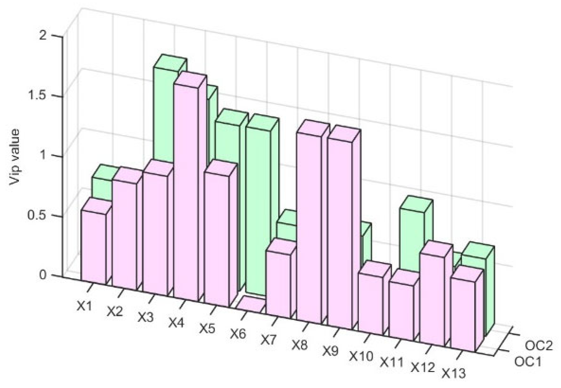
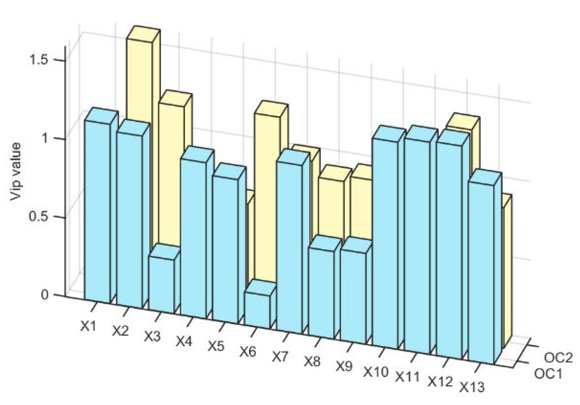
All feature extraction methods use the prediction network proposed in this study. For different OC of each dataset, the relationship between variables will change, so that some variables with high correlation in the previous OC may not be used as the input of the next OC and vice versa. As shown in Figure 2 and Figure 3, the change in variable importance projection (VIP) of each variable when the partial least squares (PLS) method is used under different OC, and the model input VIP value usually needs to be greater than 1.
As shown in Table 2 and Table 3, the IANN method performed less effectively than the other comparison methods in variable selection, as the latter methods all successfully identified the correct variable sets. In the ETN dataset, the IANN selected irrelevant variables X1 and X4 besides the eight relevant variables, and the mRMR eliminated a redundant variable X8 to obtain a faster convergence rate. In the ETP dataset, the IANN selected the irrelevant variable X9.
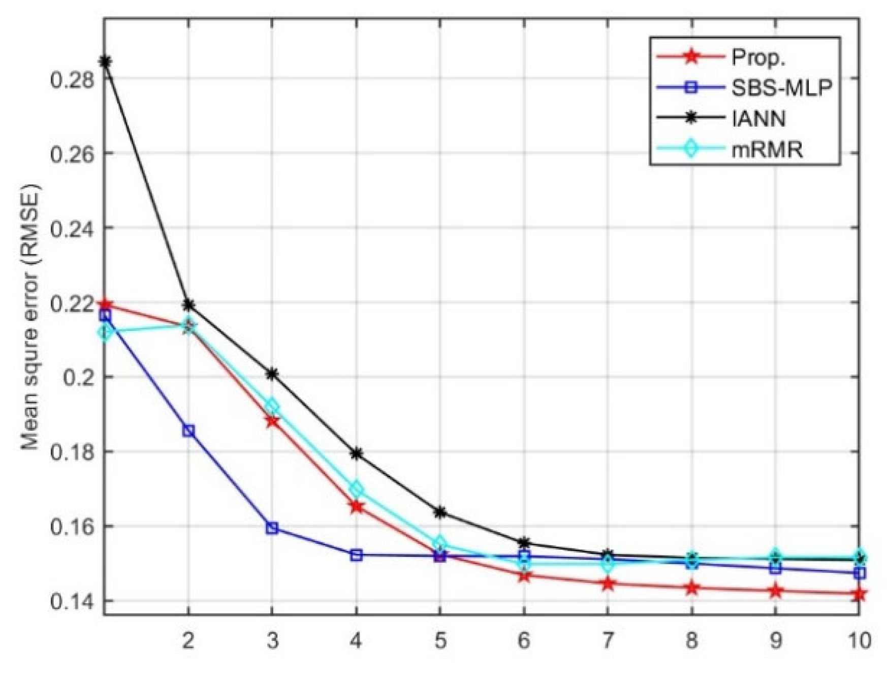
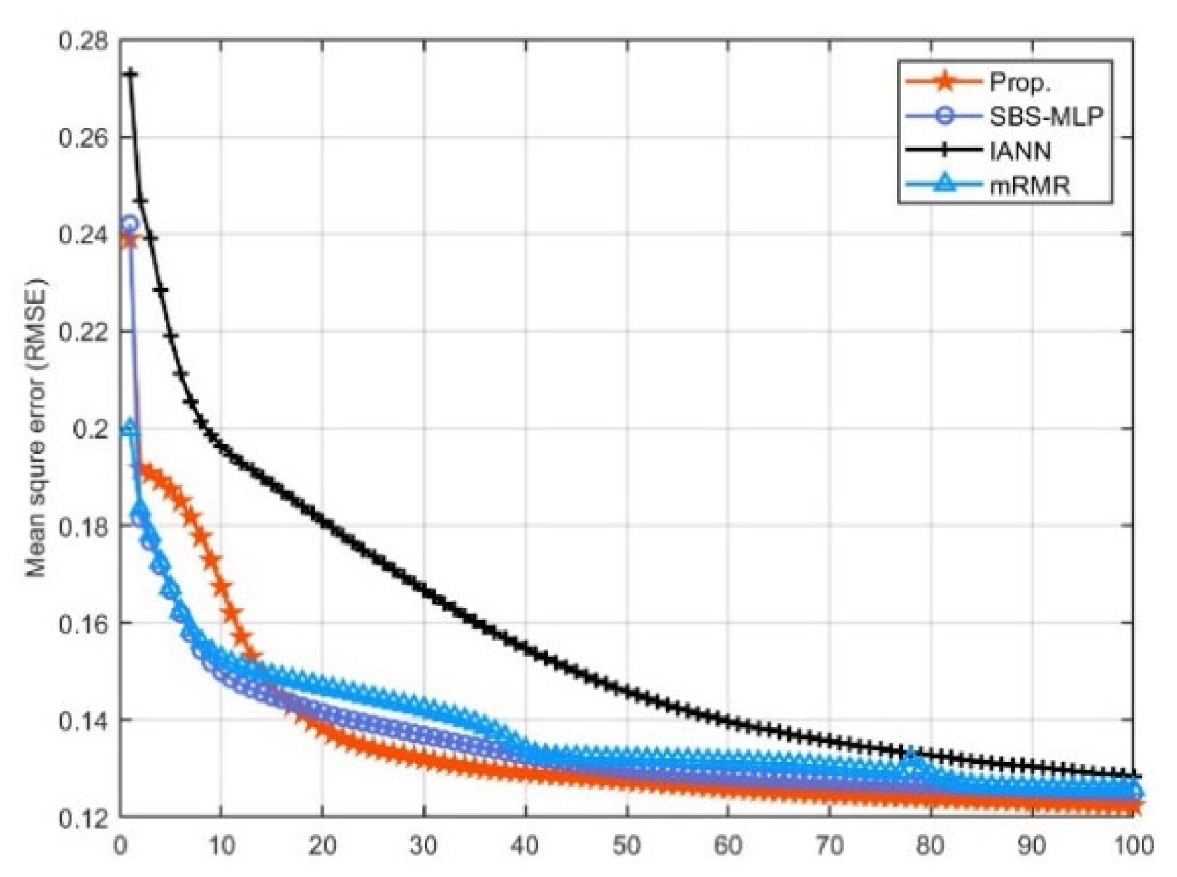
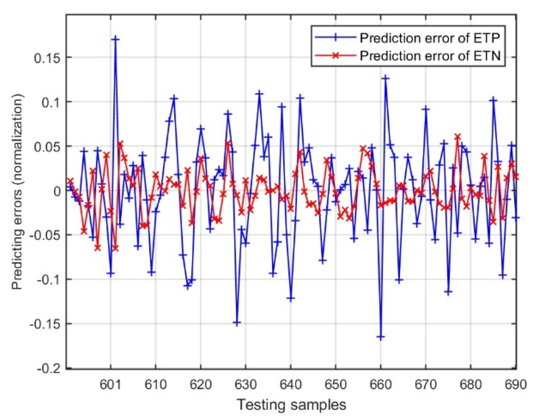
The results in Table 2 indicate that this feature selection method-based MLP can obtain high mean accuracy and faster CPU time. The results of Error rates on the ETN and ETP test dataset are displayed in Figure 4 and Figure 5, respectively. When employing a consistent set of input variables, the proposed method demonstrates comparable generalization performance on the test data to the examined methods, such as SBS-MLP, NMIFS, and mRMR. The experimental results align with expectations: IANN exhibits overfitting due to the introduction of irrelevant variables, which results in degraded performance on the test set. In contrast, SBS-MLP demonstrates the highest computational complexity, followed by the proposed method and IANN, while NMIFS and mRMR exhibit the fastest computational speeds. To validate the statistical significance of the performance improvement in the proposed ISSM, a paired t-test was conducted against the baseline method, IANN, based on the absolute prediction error across all samples in the test set. In Task A, the error difference between ISSM and IANN exhibited high statistical significance (t(99) ≈ 3.39, p < 0.001). In Task B, an equally significant performance advantage was observed (t(99) ≈ 3.85, p < 0.001). These results strongly indicate that the observed reduction in RMSE for ISSM does not stem from random fluctuations but rather from inherent performance advantages of the model itself.

4.3. Experiment II: Comparison of Self-Organizing Algorithms

To quantify the model’s fitting performance, this experiment introduces the Average Percentage Error (APE) as a performance metric. The calculation method for this metric is as follows:
A P E = 1 T t = 1 T y d ( t ) g ^ ( t ) y d ( t ) × 100 % .
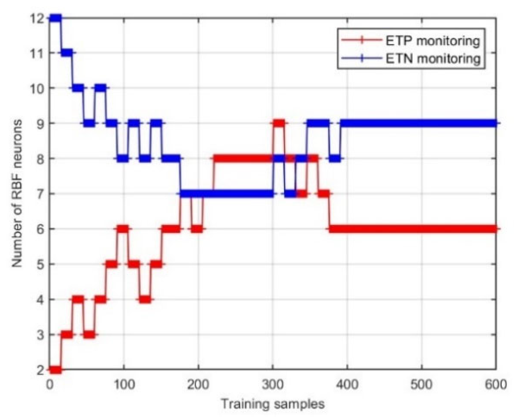
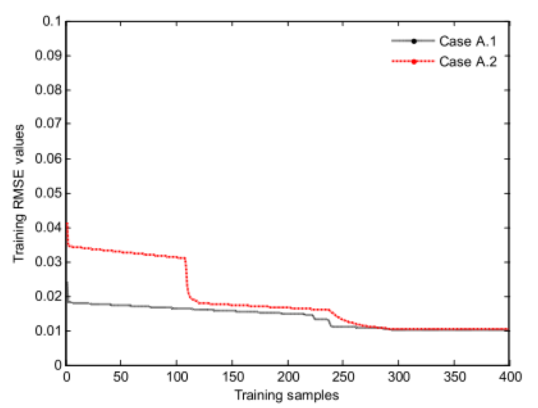
The simulation results validate the outstanding performance of the F-FNN model. Figure 6 reveals the dynamic changes in the number of ETP and ETN neurons during training. Figure 7 illustrates the decline process of the training mean-squared error. The results demonstrate that this model exhibits exceptional dynamic system approximation capabilities for datasets with varying open-loop errors. As shown in Figure 6, the F-FNN model exhibits asymptotic convergence over the first 300 samples but subsequently overfits, which signals a decline in its generalization performance. After applying feature selection, this issue is effectively controlled, ultimately enabling the network to achieve excellent operating condition transfer performance.
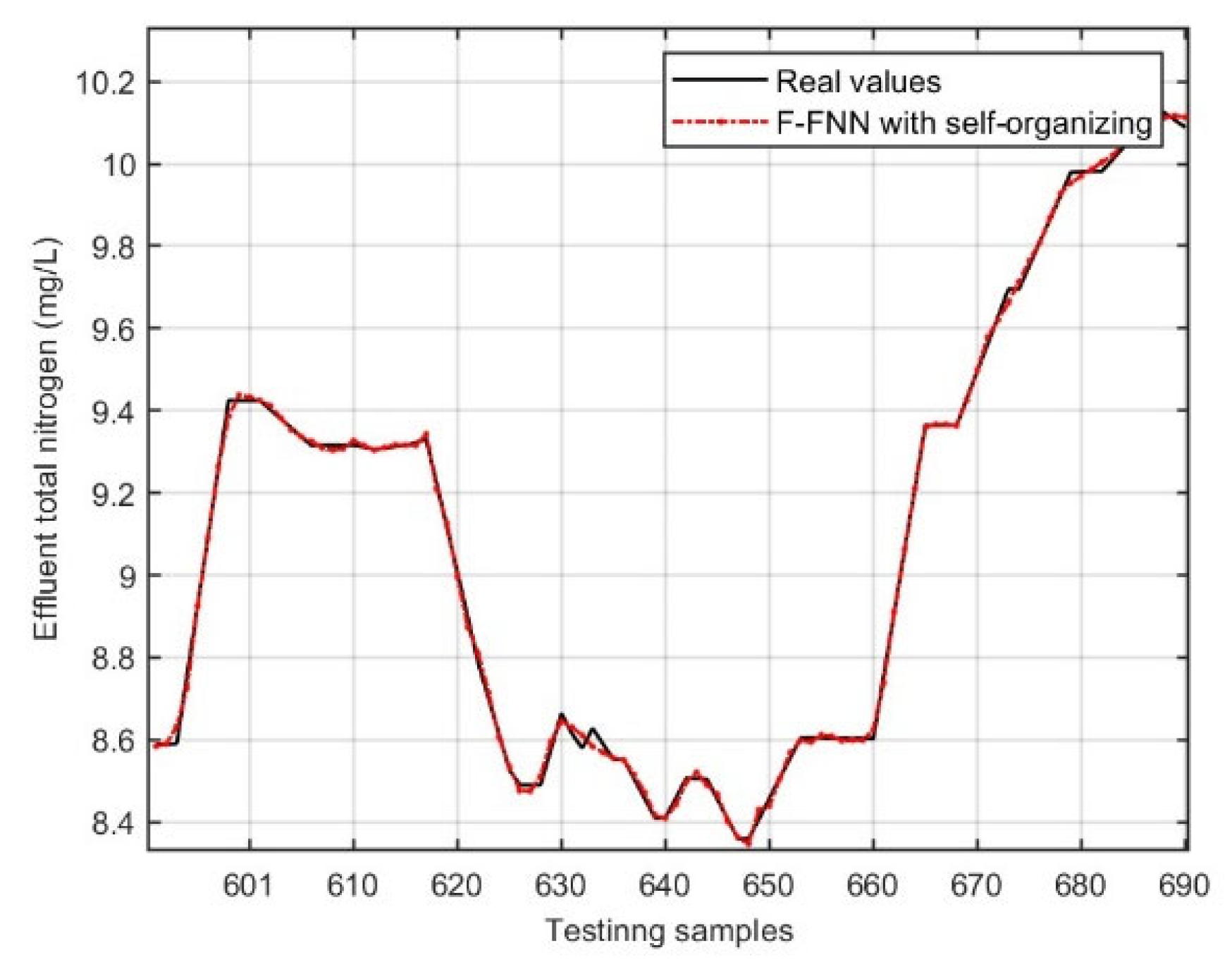
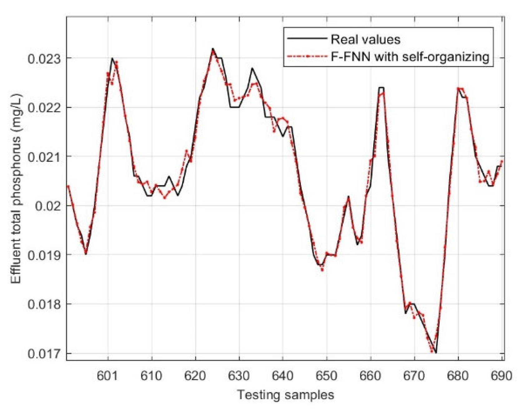
Figure 8 and Figure 9, respectively, demonstrate the model’s predictive performance for monitoring effluent total phosphorus (ETP) and effluent total nitrogen (ETN). As shown, the self-organizing F-FNN closely tracks the fluctuation trends of actual values in both ETP and ETN test samples. Specifically, the model accurately reproduces the trends in water quality parameters and captures multiple rapidly changing fluctuation peaks and troughs (e.g., the abrupt change points near sample numbers 610 and 660 in Figure 9). This fully demonstrates that F-FNN possesses outstanding nonlinear dynamic system modeling capabilities, which can effectively learn and approximate the complex nonlinear dynamic characteristics in WWTP. To quantitatively evaluate its performance, this study compares F-FNN with several advanced algorithms, including the Self-Organizing Fuzzy Neural Network Adaptive Computation Algorithm (SOA-SOFNN) [50], DFNN [42], GDFNN [51], SOFMLS [52], and GP-FNN [53]. To ensure fairness in the comparison, all methods employed identical training data.
The parameter settings for this experiment are as follows: the initial number of RBF neurons in ETP and ETN is 2 and 12, respectively. The effluent water quality is evaluated using a permissible error of 0.1 mg/L, while the model’s generalization performance is comprehensively assessed based on the average test root mean square error (RMSE) and average prediction accuracy. Figure 8, Figure 9 and Figure 10, respectively, display the predicted effluent concentration results and their corresponding prediction errors. To comprehensively evaluate the performance of the F-FNN, Table 3 further compares its network structure, average test RMSE, and prediction accuracy with multiple methods. The data in the table represent the average of 30 independent trials.
As shown in Table 3, the self-organizing F-FNN achieved the highest average prediction accuracy. Its precision significantly outperformed fixed-structure F-FNN, DFNN, GDFNN, GP-FNN, and traditional mathematical models [13]. This demonstrates that the proposed self-organizing F-FNN effectively enhances the accuracy of wastewater quality monitoring.

4.4. Experiment III: Comparison of Parameter Update Mode

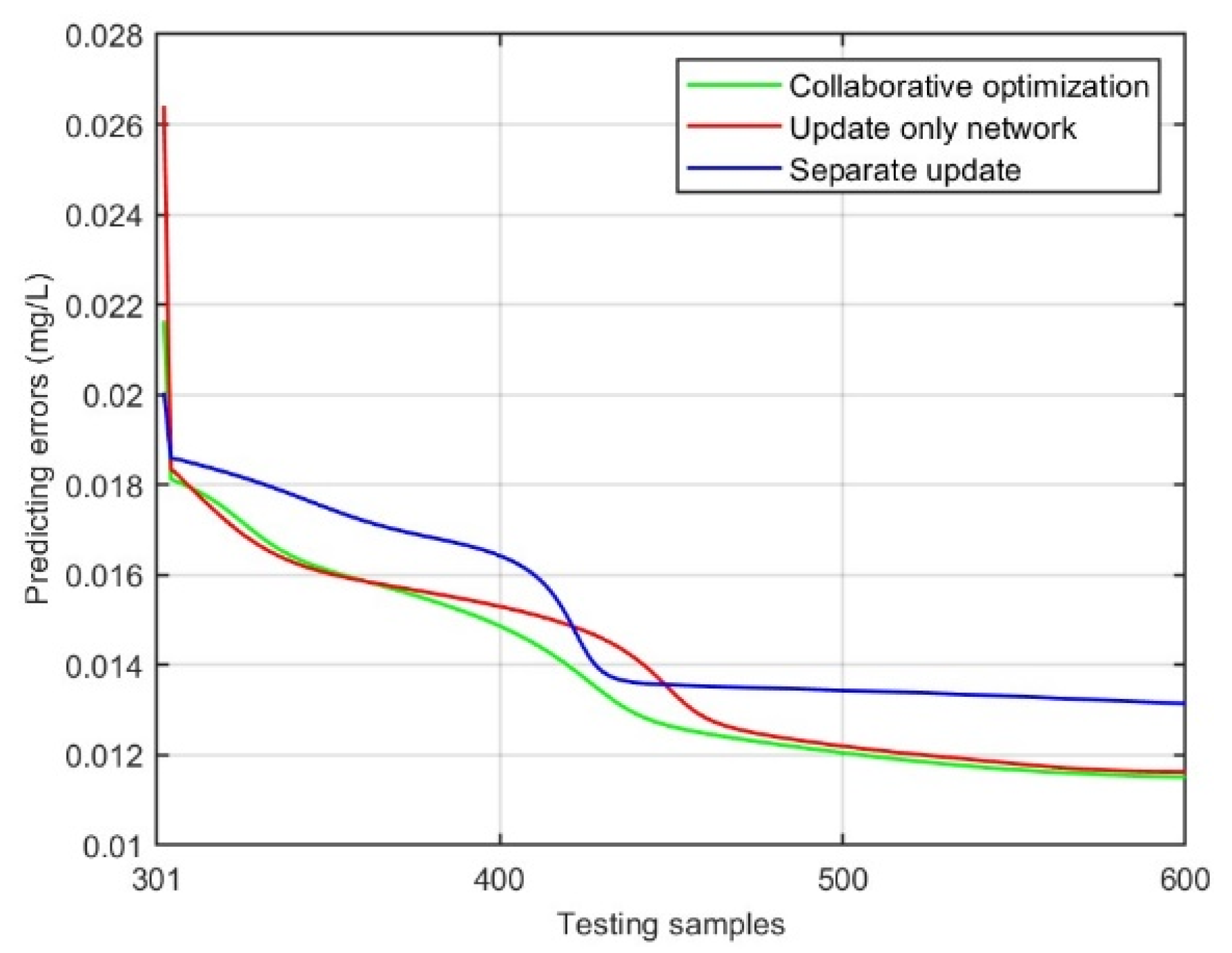
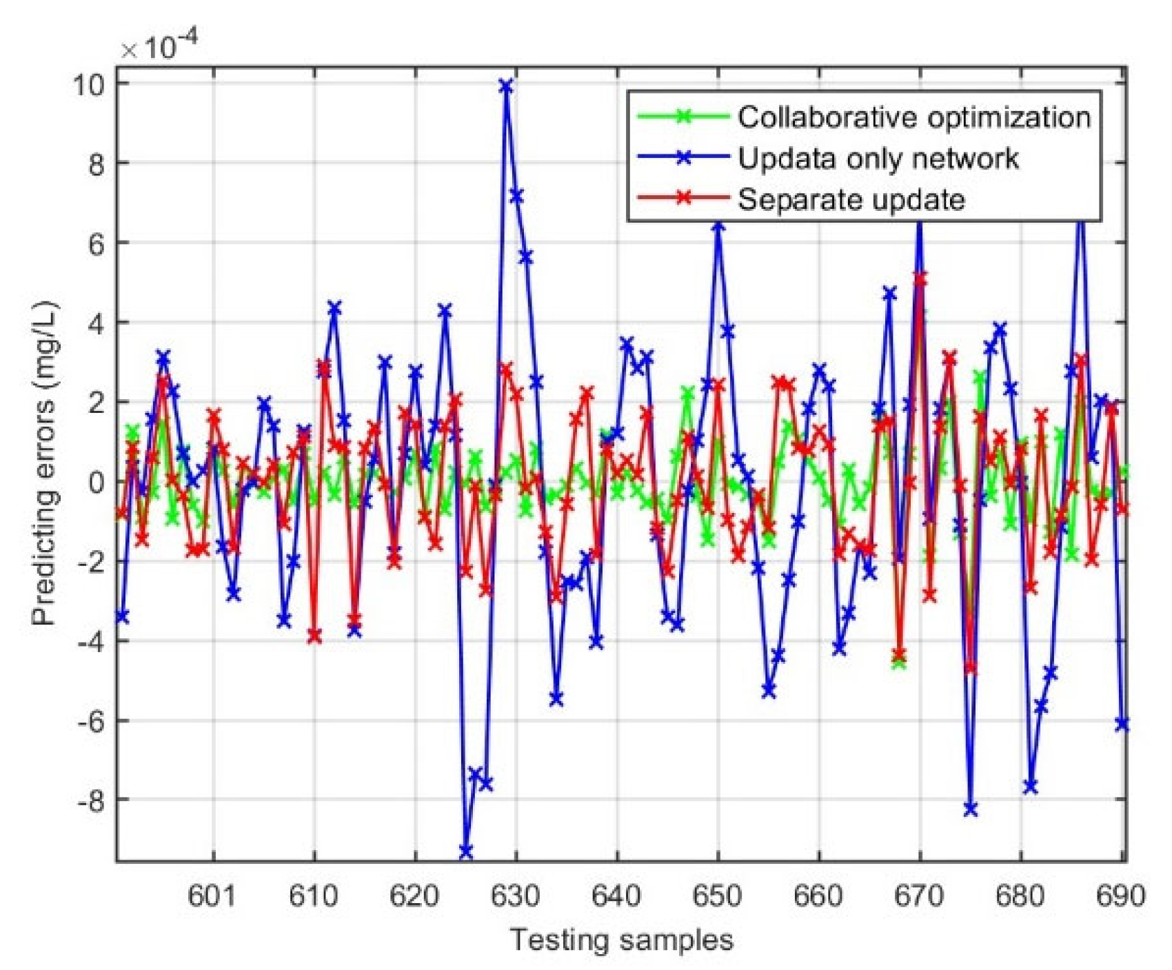
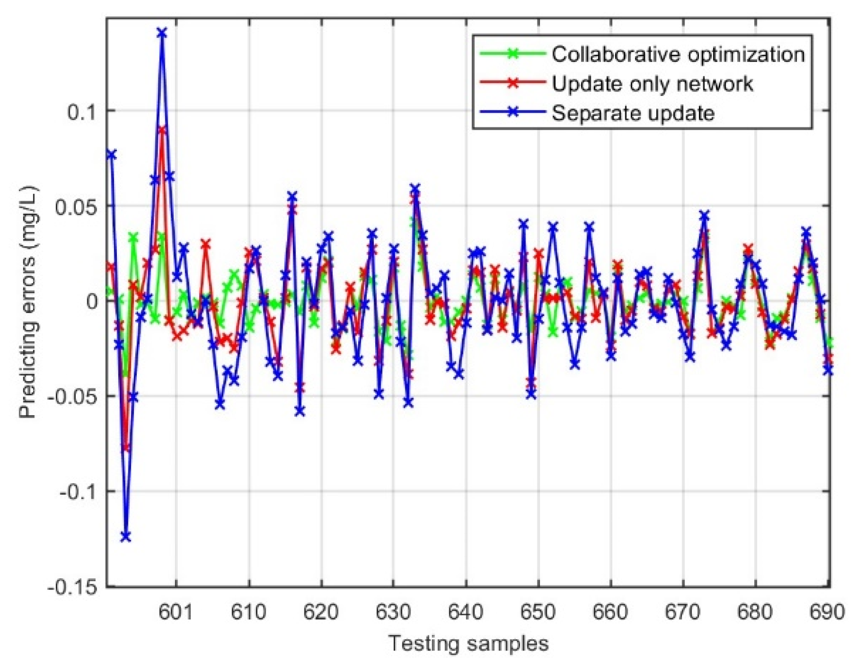
To evaluate the performance of the collaborative optimization algorithm, the experiment compares differences between only updating network parameters, separately updating parameters, and collaborative updating parameters, and distinguishes the advantages and disadvantages of each mode by RMSE and mean accuracy. Three different parameter update modes correspond to three feature extraction modes of soft sensor offline, filter, and embedded.
The modeling capabilities and convergence performance of the three modes are shown in Figure 11, which indicates that SSM exhibits acceptable convergence. The testing errors for ETP and ETN are presented in Figure 12 and Figure 13, respectively, with more detailed data recorded in Table 3. All results consistently demonstrate that the collaborative parameter update mode significantly outperforms the other two modes in both prediction accuracy and operational stability. This mode ensures that parameters of both the feature extraction layer and the feature representation layer are adjusted in a coordinated manner, using a re-weighted regularized conjugate gradient method. This coordination helps suppress abrupt changes in the parametric space, leading to smoother model adaptation and improved real-time monitoring performance.
In contrast, updating parameters only or separately can lead to suboptimal performance, as these modes do not account for the interdependencies between different layers of the network. The collaborative update mode, by considering these interdependencies, achieves a more balanced and effective optimization, resulting in higher mean accuracy and lower RMSE values. This experiment underscores the importance of a holistic approach to parameter calibration in dynamic systems like WWTPs.

5. Conclusions

This study introduces an innovative ISSM tailored specifically for the dynamic and complex environment of WWTPs. The ISSM stands out due to its unique collaborative calibration strategy, which enables the model to adapt its structure and parameters online in response to changing input variables and operating conditions. This self-organizing capability ensures that the ISSM maintains high monitoring accuracy and stability, even under scenarios characterized by concept drift and sudden operational changes.
One of the key strengths of the ISSM lies in its ability to perform dynamic feature extraction and selection, ensuring that only the most relevant input variables are considered. This reduces computational overhead while enhancing the model’s predictive performance. Furthermore, the collaborative optimization algorithm employed in the ISSM allows for simultaneous calibration of front and back network parameters, promoting a balanced trade-off between accuracy and computational efficiency.
Experimental results demonstrate that compared to existing methods, ISSM exhibits significant overall performance advantages in adaptability, accuracy, and real-time capability. Compared to traditional methods, accuracy has improved by over 5%, while computational speed has increased by more than threefold while maintaining precision. By effectively addressing the challenges posed by the dynamic nature of WWTPs, the ISSM offers a reliable and cost-effective solution for ensuring compliance with environmental regulations and optimizing treatment process efficiency.
In conclusion, the ISSM and its collaborative calibration strategy have marked a considerable improvement in WWTP monitoring, with broad potential applications in other complex industrial processes. A key future direction is to test its performance under complex operating conditions involving full-process and multi-unit operations in series.

Author Contributions

Methodology, Y.Y.; Validation, X.W.; Investigation, X.W. and Y.Y.; Data curation, X.W. and Y.Z.; Writing—original draft, Y.Z. and Y.Y.; Project administration, Y.Y. All authors have read and agreed to the published version of the manuscript.

Funding

This work was funded by the National Science Foundation of China under Grants 62422301, 62125301, and 92467205, National Key Research and Development Project under Grants 2022YFB3305800-05, Beijing Nova Program under Grant Z211100002121073, and Youth Beijing Scholar under Grant No. 037.

Data Availability Statement

The data presented in this study are available on request from the corresponding author. The data are not publicly available due to the protection of data privacy and intellectual property rights.

Conflicts of Interest

All the authors declare that they have no competing financial interests or personal relationships that could influence the work reported in this paper.

References

  1. Yan, R.; Han, J.; Shen, G.; Hao, Z.; Han, Y.; Xiong, W.; Liang, B.; Gao, S.; Yang, M.; Sun, Y.; et al. The threat of PPCPs from WWTP and solutions of advanced reduction coupled treatment processes with pilot-scale. J. Hazard. Mater. 2025, 498, 139782. [Google Scholar] [CrossRef] [PubMed]
  2. Jin, H.-T.; Xu, K.; Ding, T.; You, A.-J.; Hu, J.-W.; Hua, L.; Gan, Z.-W.; Hu, L.-F. Kitchen waste composting leachate stimulates endogenous simultaneous nitrifying and denitrifying pathways in WWTPs. Environ. Res. 2025, 285, 122588. [Google Scholar] [CrossRef] [PubMed]
  3. Chen, Q.Y.; Yu, L.-F.; Yu, T.; Fan, Y.; An, M.-Z.; Tian, X. Flow partitioning strategy for partial denitrification and anammox (PD/A) implementation: Simultaneous treatment of raw sewage and secondary effluent in WWTPs. J. Water Process Eng. 2025, 77, 108276. [Google Scholar] [CrossRef]
  4. Qiao, J.-F.; Zhang, J.-N.; Li, W.-J. PCA-based sensor drift fault detection with distribution adaptation in wastewater treatment process. IEEE Trans. Autom. Sci. Eng. 2025, 22, 10071–10083. [Google Scholar] [CrossRef]
  5. Han, H.-G.; Xu, Z.-A.; Wang, J.-J. A novel set-based discrete particle swarm optimization for wastewater treatment process effluent scheduling. IEEE Trans. Cybern. 2024, 54, 5394–5406. [Google Scholar] [CrossRef]
  6. Li, J.; Wang, J.-L.; Sui, E.-G.; Wang, W.; He, R. Soft sensor development based on hybrid modeling with ensemble learning for multimode batch processes. IEEE Sens. J. 2025, 25, 15588–15597. [Google Scholar] [CrossRef]
  7. Gao, S.-W.; Li, T.-Z.; Dong, X.-H.; Dang, X.-C. Semi-supervised soft sensor modeling based on ensemble learning with pseudo label optimization. IEEE Trans. Instrum. Meas. 2024, 73, 2524818. [Google Scholar] [CrossRef]
  8. Yuan, X.-F.; Xu, N.; Ye, L.-J.; Wang, K.; Shen, F.-F.; Wang, Y.-L. Attention-Based Interval Aided Networks for Data Modeling of Heterogeneous Sampling Sequences with Missing Values in Process Industry. IEEE Trans. Ind. Inform. 2024, 20, 5253–5262. [Google Scholar] [CrossRef]
  9. Ba-Alawi, A.-H.; Kim, J. Dual-stage soft sensor-based fault reconstruction and effluent prediction toward a sustainable wastewater treatment plant using attention fusion deep learning model. J. Environ. Chem. Eng. 2025, 13, 116221. [Google Scholar] [CrossRef]
  10. Dias, A.-L.; Turcato, A.-C.; Sestito, G.-S. A soft sensor edge-based approach to fault diagnosis for piping systems. Flow Meas. Instrum. 2024, 97, 102618. [Google Scholar] [CrossRef]
  11. Jiang, D.-N.; Yang, H.-W.; Cao, H.-C.M.; Xu, D.-Z. A missing data imputation method for industrial soft sensor modeling. J. Process Control. 2025, 152, 103485. [Google Scholar] [CrossRef]
  12. Hu, H.-S.; Feng, D.-Z.; Yang, F. A promising nonlinear dimensionality reduction method: Kernel-based within class collaborative preserving discriminant projection. IEEE Signal Process. Lett. 2020, 27, 2034–2038. [Google Scholar] [CrossRef]
  13. Louifi, A.; Kouadri, A.; Harkat, M.-F.; Bensmail, A.; Mansouri, M. Sensor fault detection in uncertain large-scale systems using interval-valued PCA technique. IEEE Sens. J. 2024, 25, 3119–3125. [Google Scholar] [CrossRef]
  14. Hu, C.-H.; Luo, J.-Y.; Kong, X.-Y.; Xu, Z.-Y. Orthogonal multi-block dynamic PLS for quality-related process monitoring. IEEE Trans. Autom. Sci. Eng. 2023, 21, 3421–3434. [Google Scholar] [CrossRef]
  15. Yin, J.-J.; Alias, A.-H.; Haron, N.-A.; Bakar, N.-A. Development of a hoisting safety risk framework based on the stamp theory and PLS-sem method. IEEE Access 2024, 12, 122998–123017. [Google Scholar] [CrossRef]
  16. Al-Emran, M.; AlQudah, A.-A.; Abbasi, G.-A.; Al-Sharafi, M.-A.; Iranmanesh, M. Determinants of using ai-based chatbots for knowledge sharing: Evidence from PLS-SEM and fuzzy sets (fsQCA). IEEE Trans. Eng. Manag. 2023, 71, 4985–4999. [Google Scholar] [CrossRef]
  17. Cheah, J.-H.; Hair, J.-F. Explaining and predicting new retail market and consumer behavior habits using partial least squares structural equation modeling (PLS-SEM). J. Retail. Consum. Serv. 2025, 87, 104446. [Google Scholar] [CrossRef]
  18. Briscik, M.; Dillies, M.-A.; Déjean, S. Improvement of variables interpretability in kernel PCA. BMC Bioinform. 2023, 24, 282. [Google Scholar] [CrossRef]
  19. Sahoo, T.-K.; Negi, A.; Banka, H. 14-Dimensionality reduction using PCAs in feature partitioning framework. In Statistical Modeling in Machine Learning; Academic Press: Cambridge, MA, USA, 2023; pp. 269–286. [Google Scholar]
  20. Huang, J.; Yan, X.-F. Related and independent variable fault detection based on KPCA and SVDD. J. Process Control. 2016, 39, 88–99. [Google Scholar] [CrossRef]
  21. Deng, X.-G.; Tian, X.-M.; Chen, S. Deep principal component analysis based on layerwise feature extraction and its application to nonlinear process monitoring. IEEE Trans. Control. Syst. Technol. 2019, 27, 2526–2540. [Google Scholar] [CrossRef]
  22. Si, Y.-B.; Wang, Y.-Q.; Zhou, D.-H. Key-performance-indicator-related process monitoring based on improved kernel partial least squares. IEEE Trans. Ind. Electron. 2020, 68, 2626–2636. [Google Scholar] [CrossRef]
  23. Wang, G.; Jiao, J.-F. A kernel least squares based approach for nonlinear quality-related fault detection. IEEE Trans. Ind. Electron. 2016, 64, 3195–3204. [Google Scholar] [CrossRef]
  24. Wei, C.-H.; Song, Z.-H. Generalized semi supervised self-optimizing kernel model for quality-related industrial process monitoring. IEEE Trans. Ind. Electron. 2020, 67, 10876–10886. [Google Scholar] [CrossRef]
  25. Cheng, T.; Dairi, A.; Harrou, F.; Sun, Y.; Leiknes, T. Monitoring Influent Conditions of Wastewater Treatment Plants by Nonlinear Data-Based Techniques. IEEE Access 2019, 7, 108827–108837. [Google Scholar] [CrossRef]
  26. Abouzari, M.; Pahlavani, P.; Izaditame, F.; Bigdeli, B. Estimating the chemical oxygen demand of petrochemical wastewater treatment plants using linear and nonlinear statistical models—A case study. Chemosphere 2021, 270, 129465. [Google Scholar] [CrossRef]
  27. Samuelsson, O.; Lindblom, E.-U.; Djupsjö, K.; Kanders, L.; Corominas, L. Mobility data for reduced uncertainties in model-based WWTP design. Water Res. X 2025, 29, 100418. [Google Scholar] [CrossRef]
  28. Yu, W.-B.; Liu, R.-B.; Zhu, K.-Y.; Hao, X.-D. Variable emission factors of CH4 and N2O from WWTPs: A model-based analysis on available data. Environ. Res. 2025, 264, 120380. [Google Scholar] [CrossRef]
  29. Wang, Y.; Li, T.; Bai, L.-M.; Yu, H.-R.; Qu, F.-S. Comparison of interpretable machine learning models and mechanistic model for predicting effluent nitrogen in WWTP. J. Water Process Eng. 2025, 77, 108344. [Google Scholar] [CrossRef]
  30. Dimitriadou, S.; Kokkinos, P.-A.; Kyzas, G.-Z.; Kalavrouziotis, I.-K. Fit-for-purpose WWTP unmanned aerial systems: A game changer towards an integrated and sustainable management strategy. Sci. Total Environ. 2024, 949, 174966. [Google Scholar] [CrossRef]
  31. Ciuccoli, N.; Fatone, F.; Sgroi, M.; Eusebi, A.-L.; Rosati, R.; Screpanti, L.; Mancini, A.; Scaradozzi, D. Forecasting and early warning system for wastewater treatment plant sensors using multitask and LSTM neural networks: A Simulated and Real-World Case Study. Comput. Chem. Eng. 2025, 198, 109103. [Google Scholar] [CrossRef]
  32. Mihály, N.-B.; Vasile, A.-V.; Cristea, M. Artificial neural networks-based identification of the WWTP DO sensor types of faults. In Computer Aided Chemical Engineering; Kokossis, A.C., Georgiadis, M.C., Pistikopoulos, E., Eds.; Elsevier: Amsterdam, The Netherlands, 2023; Volume 52, pp. 1879–1884. [Google Scholar]
  33. Karadimos, P.; Anthopoulos, L. Development of artificial neural networks for predicting the construction costs of WWTPs in Greece. Procedia Comput. Sci. 2025, 263, 285–292. [Google Scholar] [CrossRef]
  34. Tan, T.-J.; Yang, Z.; Chang, F.; Zhao, K. Prediction of the first weighting from the working face roof in a coal mine based on a GA-BP neural network. Appl. Sci. 2019, 9, 4159. [Google Scholar] [CrossRef]
  35. Nourani, V.; Elkiran, G.; Abba, S.I. Wastewater treatment plant performance analysis using artificial intelligence-an ensemble approach. Water Sci. Technol. 2018, 78, 2064–2076. [Google Scholar] [CrossRef] [PubMed]
  36. Singh, N.-K.; Yadav, M.; Singh, V.; Padhiyar, H.; Kumar, V.; Bhatia, S.-K.; Show, P.-L. Artificial intelligence and machine learning-based monitoring and design of biological wastewater treatment systems. Bioresour. Technol. 2023, 369, 128486. [Google Scholar] [CrossRef] [PubMed]
  37. Xu, B.; Pooi, C.-K.; Tan, K.-M.; Huang, S.-J.; Shi, X.-Q.; Ng, H.-Y. A novel long short-term memory artificial neural network (LSTM)-based soft-sensor to monitor and forecast wastewater treatment performance. J. Water Process Eng. 2023, 54, 104041. [Google Scholar] [CrossRef]
  38. Qiao, J.-F.; Chen, D.; Yang, C.; Li, D. Double-Layer Fuzzy Neural Network Based Optimal Control for Wastewater Treatment Process. IEEE Trans. Fuzzy Syst. 2025, 33, 2062–2073. [Google Scholar] [CrossRef]
  39. Liu, Z.; Han, H.; Yang, H.; Qiao, J. Knowledge-Aided and Data-Driven Fuzzy Decision Making for Sludge Bulking. IEEE Trans. Fuzzy Syst. 2023, 31, 1189–1201. [Google Scholar] [CrossRef]
  40. Meng, X.; Zhang, Y.; Quan, L.-M.; Qiao, J.-F. A self-organizing fuzzy neural network with hybrid learning algorithm for nonlinear system modeling. Inf. Sci. 2023, 642, 119145. [Google Scholar] [CrossRef]
  41. Campos, P.-V. Fuzzy neural networks and neuro-fuzzy networks: A review the main techniques and applications used in the literature. Appl. Soft Comput. 2020, 92, 106275. [Google Scholar] [CrossRef]
  42. Winkler, M.-K.; Ettwig, K.-F.; Vannecke, T.-P.; Stultiens, K.; Bogdan, A.; Kartal, B.; Volcke, E.-I.-P. Modelling simultaneous anaerobic methane and ammonium removal in a granular sludge reactor. Water Res. 2015, 73, 323–331. [Google Scholar] [CrossRef]
  43. Harrou, F.; Cheng, T.; Sun, Y.; Leiknes, T.; Ghaffour, N. A Data-Driven Soft Sensor to Forecast Energy Consumption in Wastewater Treatment Plants: A Case Study. IEEE Sens. J. 2021, 21, 4908–4917. [Google Scholar] [CrossRef]
  44. Cao, J.-F.; Xue, A.; Yang, Y.; Cao, W.; Hu, X.-J.; Cao, G.-L.; Gu, J.-H.; Zhang, L.; Geng, X.-L. Deep learning based soft sensor for microbial wastewater treatment efficiency prediction. J. Water Process Eng. 2023, 56, 104259. [Google Scholar] [CrossRef]
  45. Ryu, K.-Y.; Sung, M.-J.; Gupta, P.-Y.; D'sa, J.; Tariq, F.-M.; Isele, D.; Bae, S.-J. IANN-MPPI: Interaction-aware neural network-enhanced model predictive path integral approach for autonomous driving. Comput. Sci. 2025, arXiv:2507.11940. [Google Scholar]
  46. Zhang, Y.; Yang, Q. A Survey on Multi-Task Learning. IEEE Trans. Knowl. Data Eng. 2022, 34, 5586–5609. [Google Scholar] [CrossRef]
  47. Sergio, R.-G.; Iago, L.; David, M.-R.; Verónica, B.-C.; José, M.-B.; Francisco, H.; Amparo, A.-B. Fast-mRMR: Fast minimum redundancy maximum relevance algorithm for high-dimensional big data. Intell. Syst. 2016, 32, 134–152. [Google Scholar]
  48. Cheng, J.-H.; Sun, J.; Yao, K.-S.; Xu, M.; Cao, Y. A variable selection method based on mutual information and variance inflation factor. Spectrochim. Acta Part A Mol. Biomol. Spectrosc. 2022, 268, 1386–1425. [Google Scholar] [CrossRef]
  49. Meng, W.; Lu, Y.-Q.; Qin, J.-C. A dynamic MLP-based DDoS attack detection method using feature selection and feedback. Comput. Secur. 2020, 88, 101645. [Google Scholar]
  50. Han, H.-G.; Zhang, L.; Wu, X.-L.; Qiao, J.-F. An efficient second-order algorithm for self-organizing fuzzy neural networks. IEEE Trans. Cybern. 2017, 49, 14–26. [Google Scholar] [CrossRef]
  51. Jahromi, A.-T.; Er, M.-J.; Li, X.; Lim, B.-S. Sequential fuzzy clustering based dynamic fuzzy neural network for fault diagnosis and prognosis. Neurocomputing 2016, 196, 31–41. [Google Scholar] [CrossRef]
  52. Feng, S.; Chen, C.-P. Fuzzy Broad Learning System: A Novel Neuro-Fuzzy Model for Regression and Classification. IEEE Trans. Cybern. 2020, 50, 414–424. [Google Scholar] [CrossRef]
  53. Huang, H.; Yang, C.; Chen, C.-P. Optimal Robot–Environment Interaction Under Broad Fuzzy Neural Adaptive Control. IEEE Trans. Cybern. 2021, 51, 3824–3835. [Google Scholar] [CrossRef]
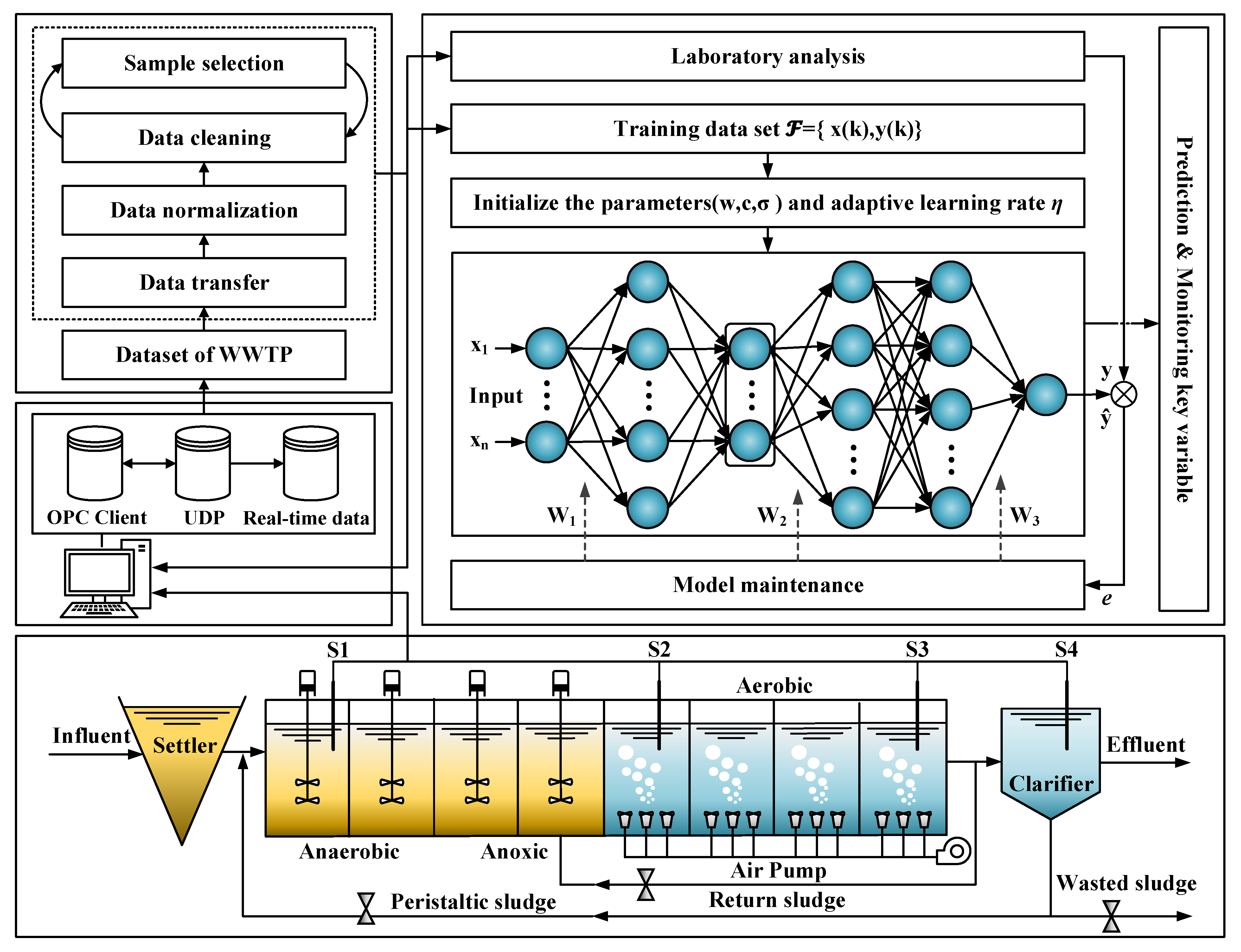
Figure 1. The ISSM-based monitoring system.
Electronics 14 04506 g001
Figure 2. Correlation changes in variables (ETP).
Electronics 14 04506 g002
Figure 3. Correlation changes in variables (ETN).
Electronics 14 04506 g003
Figure 4. Error rates on the ETN test dataset.
Electronics 14 04506 g004
Figure 5. Error rates on the ETP test dataset.
Electronics 14 04506 g005
Figure 6. Number of RBF neurons in task A and task B.
Electronics 14 04506 g006
Figure 7. Training RMSE values in task A and task B.
Electronics 14 04506 g007
Figure 8. The predicted results in ETP.
Electronics 14 04506 g008
Figure 9. The predicted results in ETN.
Electronics 14 04506 g009
Figure 10. Modeling errors versus testing samples.
Electronics 14 04506 g010
Figure 11. Training RMSE values.
Electronics 14 04506 g011
Figure 12. Testing errors in ETP.
Electronics 14 04506 g012
Figure 13. Testing errors in ETN.
Electronics 14 04506 g013
Table 1. Process variables of the WWTP dataset.
VariableDescriptionUnitCollecting Points
X1Inlet flowLMPInfluent Tank
X2Temperature°CTank A
X3ORP1mVAnaerobic tank (tank A)
X4ORP2mVAnoxic tank (tank A)
X5MLSS1mg/LAnoxic tank (tank A)
X6NO3-Nmg/LAnoxic tank (tank A)
X7NH4-Nmg/LAerobic tank (tank A)
X8DO1mg/LAerobic tank (tank A)
X9ORP3mVAnaerobic tank (tank B)
X10MLSS2mg/LAnoxic tank (tank B)
X11NO3-Nmg/LAnoxic tank (tank B)
X12DO2mg/LAerobic tank (tank B)
X13pHSettler
Yd1TPmg/LSettler (effluent)
Yd2TNmg/LSettler (effluent)
Table 2. Performance comparison of different methods in Example 1.
AlgorithmTask A: Effluent Total Phosphorus MonitoringTask B: Effluent Total Nitrogen Monitoring
⎸S⎹CPU
Time(s)
Testing RMSECC⎸S⎹CPU
Time(s)
Testing RMSECC
Prop.7-64.10.14170.846-838.40.12210.8657
IANN9-86.70.15860.827-947.60.12860.8406
SBS-MLP7-61050.14980.876-8116.30.12370.8708
NMIFS7-60.1250.15310.836-810.210.12620.8539
mRMR7-60.1390.15670.846-88.90.12570.8572
Table 3. Performance comparisons between different algorithms in Example 2.
AlgorithmTask A: Effluent Total Phosphorus MonitoringTask B: Effluent Total Nitrogen Monitoring
No. of Final RBF NeuronsCPU
Time(s)
Testing RMSETesting
APE
No. of Final RBF NeuronsCPU
Time(s)
Testing RMSETesting
APE
Prop.621.610.01520.0043952.210.1330.052
Prop (fixed structure)224.550.02320.01021240.120.1980.083
SOA-FNN611.270.01050.0031928.640.0570.010
DFNN636.550.01240.0039882.120.1650.067
GDFNN842.330.02170.00849142.670.1780.081
GP-FNN628.240.01050.0046989.310.1820.092
SOFMLS829.360.01200.0095978.630.1930.098
Disclaimer/Publisher’s Note: The statements, opinions and data contained in all publications are solely those of the individual author(s) and contributor(s) and not of MDPI and/or the editor(s). MDPI and/or the editor(s) disclaim responsibility for any injury to people or property resulting from any ideas, methods, instructions or products referred to in the content.