Article

Research on Hybrid Optimization Prediction Models for Photovoltaic Power Generation Under Extreme Climate Conditions

1
Jiangmen Power Supply Bureau, Guangdong Power Grid Co., Ltd., Jiangmen 529000, China
2
School of Electric Power Engineering, South China University of Technology, Guangzhou 510641, China
*
Authors to whom correspondence should be addressed.
Electronics 2025, 14(22), 4475; https://doi.org/10.3390/electronics14224475 (registering DOI)
Submission received: 26 September 2025 / Revised: 7 November 2025 / Accepted: 12 November 2025 / Published: 17 November 2025

Abstract

With the vigorous development of contemporary clean energy, the participation rate of photovoltaic (PV) power generation in the whole power system is increasing day by day, and accurate PV power prediction technology is crucial for the optimal scheduling of the power system. However, the frequent occurrence of extreme climate in recent years has caused greater disturbance to PV power generation, which greatly increases the degree of difficulty in accurately predicting PV power generation and thus affects the security, economy, reliability and stability of grid system operation. In order to predict PV power under extreme climatic conditions, we firstly elaborate the PV power prediction methods and their respective advantages and disadvantages for sand, dust, rainstorm and snowfall in existing studies, and on this basis, we propose the Gray Wolf Optimization for Short-Term Forecasting Models of the Long and Short-Term Memory Model based on K-Means clustering, which ensures the accuracy of PV power prediction under extreme climatic conditions. power prediction accuracy under extreme climate conditions. Firstly, the K-means clustering algorithm is utilized to perform weather typing, which is divided into four weather categories, namely, dusty weather, heavy rain, heavy snow and normal weather. Then, for the weather typing results, the prediction effects of the Gray Wolf Optimization Long Short-Term Memory Network (GWO-LSTM) Model, Random Forest (RF) Model, Multilayer Feedforward Neural Network (BP) Model, and Long and Short-Term Memory Network (LSTM) Model are compared, respectively. The prediction results indicate that GWO-LSTM achieves the highest forecasting accuracy, with a mean root mean square error (RMSE) of 0.6235 across all four weather scenarios. Its prediction accuracy reaches approximately 95%, providing effective data support for the safe and stable operation of new power systems featuring high proportions of grid-connected photovoltaic generation.

1. Introduction

As the global traditional fossil energy market deficit continues to expand and the degree of environmental pollution continues to increase, the energy crisis and environmental problems are becoming more prominent. In recent years, socio-economic development and energy supply have become more and more closely linked, and photovoltaic power generation has become a mainstream means of coping with the energy crisis in the world. Currently, under the strong support of various policies, PV power generation technology is developing rapidly in China, and the relevant installed capacity ranks first in the world. By the first half of 2025, China’s new photovoltaic (PV) installed capacity had grown by 99.3% year-on-year, accounting for approximately 91.5% of all new installations. Cumulative installed capacity reached about 110 gigawatts, a 54.1% increase from the previous year, representing 59.2% of the nation’s total power generation capacity. Distributed PV once again emerged as the primary driver of market growth, contributing over half of the new installations, primarily concentrated in resource-rich regions such as Xinjiang and Inner Mongolia. According to the National Energy Administration, after years of development, China has become the world’s largest investor in photovoltaic power generation, possessing unparalleled market competitiveness and potential compared to other countries. However, PV power generation is greatly affected by the meteorological environment; there is greater randomness and volatility, humidity, temperature and wind speed and other meteorological factors will have greater interference in the PV power generation prediction, and different types of weather brought about by the meteorological characteristics of the difference to the PV power generation and the grid pose a serious challenge.
Currently, for predicting photovoltaic power generation, heuristic algorithms are commonly employed to optimize prediction models, aiming for rapid convergence and accurate forecasting [1]. Reference [2] proposed a multi-step photovoltaic power generation prediction model based on Time Convolutional Neural Networks (TCN) and DLinear. This model achieves power prediction by utilizing an improved adaptive white noise complete set empirical mode decomposition for multivariate meteorological sequences and employing TCN to model local temporal information. Reference [3] proposes a photovoltaic power forecasting method based on an enhanced Long Short-Term Memory (LSTM) neural network. It analyzes meteorological features strongly correlated with photovoltaic power output, reduces feature data to two dimensions using a t-distribution, and ultimately trains an LSTM neural network prediction model. Reference [4] proposes a hybrid convolutional neural network (CNN) and long short-term memory model for photovoltaic power generation forecasting. CNN establishes spatial correlations between regions, while LSTM captures temporal dependencies in power data to enable prediction. Reference [5] constructs a short-term photovoltaic power forecasting model using a time-series convolutional neural network with feature extraction based on Random Forest (RF). RF is employed to calculate the contribution of each meteorological feature to power generation for key feature selection. Finally, the key meteorological features and raw power data are used in a combined model for prediction. Reference [6] proposed a correction method for photovoltaic power availability prediction based on Hidden Markov Models, achieving sequential monthly prediction correction through longitudinal same-month recursion. Reference [7] proposes a short-term PV power forecasting method integrating adaptive white noise-enhanced complete empirical mode decomposition (CEEMEDAN), least squares support vector machine (LSSVM), and autoregressive integrated moving average (ARIMA) models. An incremental search method enhances LSSVM, enabling adaptive selection of suitable input features. Reference [8] proposes a forecasting model based on Sequential Variational Modal Decomposition (SVMD) and an improved Dung Beetle Optimization Algorithm (IDBO) to optimize Kernel Extreme Learning Machine (KELM). IDBO is applied to enhance KELM, constructing the IDBO-KELM forecasting model. In summary, current approaches primarily employ machine learning, deep learning, neural networks, or hybrid algorithms for short-term photovoltaic power forecasting. However, these methods suffer from uneven initial population distributions, susceptibility to local optima, and insensitivity to extreme meteorological data, resulting in poor prediction performance under extreme weather conditions.
In summary, it is necessary to incorporate extreme meteorological factors alongside conventional meteorological elements, combining appropriate variables as input data for photovoltaic power generation forecasting models to enhance prediction accuracy. To address the aforementioned challenges, this paper proposes a GWO-LSTM model based on K-Means clustering. By comparing its predictive performance against random forest (RF) models, multi-layer feedforward neural network (BP) models, and long short-term memory (LSTM) models, this study provides practical guidance for real-world photovoltaic forecasting engineering applications. First, preprocessed weather data undergoes classification through a clustering module, with key climate factors identified via Pearson correlation analysis. Subsequently, within the long short-term memory (LSTM) network module, the gray wolf optimization module automatically adjusts network parameters to train the prediction model based on distinct weather cluster outcomes. Finally, photovoltaic forecasting is achieved using the model tailored to the corresponding climate type for that day. This model comprehensively addresses the complexity and coupling issues among multiple variables in extreme weather data [9]. By leveraging the long-term dependency capture capabilities of long short-term memory networks and further enhancing them with the gray wolf optimization algorithm, the model achieves more stable and high-precision predictions when handling complex, dynamic multivariate data. It provides effective data support for the safe and stable operation of new power systems featuring a high proportion of photovoltaic grid connections.

2. Common Photovoltaic Power Forecasting Methods Under Extreme Climate Conditions

Photovoltaic power forecasting is a critical research area in the renewable energy sector, centered on establishing models using historical data and environmental factors to predict future power generation from photovoltaic systems. Photovoltaic power forecasting techniques employ diverse methods and approaches, with most models for extreme weather conditions building upon foundational forecasting models through proposed improvements. This section will separately examine photovoltaic power forecasting methods under dust storms, heavy rainfall, and snowfall conditions, as well as their respective advantages and disadvantages, based on existing research.

2.1. Photovoltaic Power Forecasting Methods Under Sandstorm Conditions

2.1.1. Multi-Layer Feedforward Neural Network Prediction Model

Under dusty conditions, photovoltaic power forecasting must comprehensively consider the dynamic effects of dust on irradiance, module surface contamination, and system efficiency. In photovoltaic power forecasting studies under dusty meteorological conditions, physical model optimization strategies often enhance the input dimensions of neural network architectures by incorporating environmental feature parameters. Specifically, researchers integrate atmospheric optical characteristics—such as dust attenuation coefficients or aerosol optical depth—as additional features within foundational neural network prediction frameworks to improve the model’s ability to characterize complex meteorological conditions.
A typical case involves a study proposing a photovoltaic daily power prediction model based on a multilayer feedforward neural network (Back Propagation, BP). This model innovatively incorporates atmospheric transmittance parameters into the input feature space, constructing a 24 h power prediction time series model using the Back Propagation (BP) algorithm [10]. Empirical analysis demonstrated that compared to the baseline neural network model that disregarded dust attenuation effects, this improved architecture reduced the root mean square error by 9.6%, validating the significant enhancement in prediction performance achieved through environmental feature fusion [11].
The backpropagation (BP) neural network, first proposed by Rumelhart and McClelland in 1986, is a multi-layer feedforward neural network based on the error backpropagation algorithm. It stands as one of the most fundamental and widely applied models in deep learning [12]. Its core principle involves continuously adjusting the weight parameters within the network to make the predicted output as close as possible to the actual value. A BP neural network consists of an input layer, one or more hidden layers, and an output layer. Each layer may contain multiple nodes. The connection state between nodes across layers is represented by weights.

2.1.2. Advantages and Disadvantages of Multi-Layer Feedforward Neural Network Prediction

Backpropagation neural networks have reached a high level of maturity in both theoretical foundations and practical performance. Their prominent advantages lie in robust nonlinear modeling capabilities and adaptive learning properties. On one hand, they can capture complex nonlinear relationships between dust concentration and power generation in photovoltaic forecasting (such as the exponential effect of transmittance decay). On the other hand, they are also suitable for modeling the dynamic coupling of multiple variables (PM2.5, wind speed, irradiance) during dust storms. However, BP neural networks also exhibit several major limitations. For instance, during gradient backpropagation in deep networks, gradients may decay or grow exponentially, making it difficult to update shallow-layer parameters. This hinders the high-frequency model updates required for photovoltaic power forecasting. Additionally, local optima traps may occur; under conditions of sudden dust changes, local optima can lead to a sudden increase in prediction errors.

2.2. Photovoltaic Power Forecasting Methods Under Rainstorm Conditions

2.2.1. Random Forest Prediction Model

Prediction models for photovoltaic power output under heavy rainfall conditions also require consideration of atmospheric transparency effects. Typically, these models involve modeling the power output of photovoltaic modules under various rainfall conditions and integrating them with other key meteorological factors. This approach constructs prediction models for photovoltaic module power output under different rainfall scenarios, enabling the assessment of how meteorological parameters like rainfall impact module power generation. Heavy rainfall is often accompanied by abrupt changes in cloud cover thickness, sudden drops in light intensity, temperature fluctuations, and rapid increases in humidity—all nonlinear factors. The impact of these variables on PV power generation does not follow a simple linear relationship.
For photovoltaic power forecasting in rainfall scenarios, a typical approach involves employing machine learning-based statistical models [13]. The core process consists of two steps: First, all historical data is categorized based on weather phenomena to identify specific weather types such as “heavy rain.” Subsequently, the most suitable artificial intelligence algorithm is selected and trained for each category. For instance, research has demonstrated how the Random Forest algorithm can be combined with weather forecasts and historical power generation data to train and establish a photovoltaic power prediction model for heavy rain conditions [14].
Random forests effectively capture complex nonlinear relationships between features and power generation by constructing multiple decision trees. The predictive advantage of random forests under heavy rainfall conditions stems from their adaptability to nonlinear, high-noise scenarios with multiple feature interactions, as well as the robustness derived from ensemble learning. A typical case study proposes establishing a cumulative prediction model using random forest algorithms based on meteorological data collected from an experimental platform. This model incorporates relevant meteorological factors alongside the previous day’s atmospheric transparency as input variables to create a photovoltaic power prediction model [15].
As a nonparametric model in supervised learning, decision trees are essentially recursive classification frameworks based on feature space partitioning. Each node in the tree represents a reference object, each branching path denotes a possible attribute value, and each leaf node corresponds to the value of the object traversed along the path from the root node to that leaf. Random forests employ bootstrap resampling techniques to repeatedly draw k samples with replacement from the original training dataset N, generating new training datasets. These datasets are then used to build n classification trees, collectively forming the random forest. This approach essentially refines the decision tree algorithm by merging multiple decision trees, each constructed from an independently sampled dataset. In detail, Figure 1 illustrates the workflow diagram of a random forest.
Suppose there are currently M decision trees and N training samples. The correct classification result for each training sample N n is denoted as S n . y m S n represents the predicted result of training sample N n under decision tree y m .
1.
For each training sample i , its weight is initially set to 1 N , i.e., W m , i = 1 N . For the current decision tree y m , after training on all samples, if its prediction differs from the actual outcome, the overall error of the random forest increases. Initially, each sample carries equal error weight, but this weight evolves as the algorithm progresses.
2.
For each decision tree, starting from the first one, repeat the following steps:
(a)
Calculate the error function:
ε m = n = 1 N w m , n I y m x m y ,   t n
(b)
Calculate the decision power of this decision tree:
α m = ln 1 ε m ε m
(c)
Update Weight:
w m + 1 , i = W m , i Z m e a m t i y m x i ,   i = 1 ,   2 ,   3 ,   ,   N
3.
For each decision tree, a corresponding decision power α is obtained, thereby enabling a more rational integration of decision trees into a random forest with superior predictive performance:
Y M x = s i g n m M α m y m x

2.2.2. Advantages and Disadvantages of Random Forest Prediction

Random forests demonstrate highly efficient nonlinear modeling and robust noise resistance in heavy rainfall photovoltaic forecasting. They can automatically identify nonlinear coupling relationships among multiple parameters such as rainfall intensity, cloud cover thickness, and wind speed. During heavy rainfall, the Gini importance score—a measure of feature significance for sudden irradiance changes—is 42% higher than that of linear models, making them well-suited for handling sensor noise commonly encountered in heavy rainfall scenarios. However, random forest models for photovoltaic power generation forecasting under heavy rainfall conditions also exhibit certain limitations. On one hand, they suffer from a rainfall lag effect, struggling to capture the temporal dependency of precipitation events (such as the cumulative impact of continuous heavy rain on module temperature). On the other hand, their predictive capability for low-probability extreme rainfall events (e.g., hourly rainfall >50 mm) is weak, as Bootstrap sampling struggles to cover rare occurrences.

2.3. Photovoltaic Power Forecasting Methods Under Snowstorm Conditions

2.3.1. Long Short-Term Memory Network Prediction Model

Physics-based photovoltaic power forecasting methods primarily achieve predictions by jointly modeling snow accumulation on PV panel surfaces and atmospheric optical properties to indirectly derive effective irradiance. These models can also be combined with key meteorological factors—such as snow depth, panel tilt angle, and snowfall duration—to describe the probability of snow accumulation on PV components, enabling real-time snow detection for photovoltaic systems.
For snowy conditions, the photovoltaic power forecasting model significantly improves prediction accuracy by incorporating snowfall data as a key input feature. The core approach involves first modifying the clear-sky model with an empirically or data-driven “snow cover loss factor”; then training a deep learning model using both this loss factor and real-time snowfall data. This method substantially enhances the model’s performance during snowy weather [16].
The predictive advantage of LSTM under snowfall conditions stems from its robust modeling capabilities for temporal dynamics, high-noise data, and nonlinear relationships. Combined with optimization algorithms and error correction techniques, its adaptability is further enhanced. Building upon this, research has proposed a multi-perspective probability-weighted LSTM model for day-ahead PV power forecasting. This model reconstructs numerical weather prediction data through a multi-perspective approach, then constructs a similarity function based on global and local relationships in historical data. This enables classification of historical daily weather types and representation of PV generation probability under snowfall conditions. Finally, integrating probability with the long short-term memory network model achieves daily power forecasting. This approach effectively mitigates the impact of extreme numerical weather on the prediction model, significantly improving the accuracy of PV power plant forecasting [17].

2.3.2. Advantages and Disadvantages of Long-Short Term Memory Networks in Prediction

Long Short-Term Memory (LSTM) networks demonstrate unique advantages in snowfall scenarios due to their temporal dependency modeling and dynamic memory gating mechanisms. They can capture the delayed effects of irradiance attenuation and temperature changes caused by continuous snowfall, such as the persistent influence of snow depth on the following day’s power generation. Additionally, through their gating units, LSTMs can automatically learn the interactions between parameters like snow depth, temperature, and wind speed, thereby avoiding the limitations of manual feature engineering. However, LSTMs exhibit strong data dependency, requiring substantial labeled snowfall event datasets. In regions with infrequent snow disasters (e.g., southern China), models are prone to overfitting due to insufficient samples. Additionally, LSTMs cannot explicitly quantify the contribution of individual physical parameters (e.g., snow depth, temperature) to power losses, undermining the reliability of grid dispatch decisions.

3. K-Means-Based GWO-LSTM Gray Wolf Optimization Prediction Model

3.1. Weather Classification Using the K-Means Clustering Algorithm

K-means clustering is a commonly used distance-based clustering algorithm. Given a specified number of clusters k , it uses the distance between data parameters as a similarity measure to ultimately partition objects with differing similarities into the corresponding k clusters. The algorithm’s objective is to minimize the total sum of distances from points within each cluster to their respective cluster centers, ensuring the smallest sum of distances between each data point and the centroid of its assigned cluster. The basic operational steps are as follows [18].
1.
Initialize cluster centers by randomly selecting K data points as initial cluster centers based on input parameters.
2.
Calculate the Euclidean distance between each data point and the initial cluster centers, then assign each point to the nearest cluster center. The Euclidean distance formula is:
dist x , c i = j = 1 d x j c i j 2
Here, x represents the data point, c i is the i -th cluster center, d is the dimension of the data, and x j and c i j denote the values of x and c i in the j -th dimension, respectively.
3.
For each cluster, recalculate its cluster center. The new cluster center is the mean of all data points within that cluster, calculated as:
c i = 1 S i x S i x
where S i is the set of data points in the i -th cluster, and S i is the number of data points in that set.
4.
Repeat the reassignment and update steps until the cluster centers no longer change significantly, meaning the distance between the new cluster centers and the old ones is less than a preset threshold.
The number of cluster centers k significantly impacts clustering results. This paper employs the elbow rule to determine the optimal number of clusters. The clustering evaluation metric used by the elbow rule is the sum of the squares of distances from all sample points in the dataset to their respective cluster centers. This metric reflects the quality of clustering outcomes across different cluster configurations, calculated as follows:
S = i = 1 k   p C i   p m i 2
In the formula,   k denotes the number of clusters formed; C i represents the i -th cluster after clustering; P denotes the data points within that cluster; m i denotes the cluster center of the i -th cluster.

3.2. GWO Gray Wolf Optimization Algorithm

The Gray Wolf Optimizer (GWO) is a swarm intelligence optimization algorithm inspired by the hunting behavior of gray wolf packs. Proposed by Mirjalili et al. in 2014 [19], it draws inspiration from the cooperative predation strategies observed in wolf packs. GWO achieves optimization by simulating the cooperative hunting mechanism of gray wolf packs [20]. This mechanism effectively balances exploration and exploitation, demonstrating strong performance in convergence speed and solution accuracy. It is now widely applied in engineering fields. The steps of the Gray Wolf Optimization algorithm are as follows:
1.
Initialization: In GWO, to mathematically simulate the social hierarchy of wolves, the optimal solution is defined as α to represent the position of the alpha wolf (first-order wolf). Consequently, the second and third optimal solutions are designated as β and δ to represent the positions of second-order and third-order wolves, respectively. The remaining candidate solutions are designated as ω to represent the positions of subordinate wolves (fourth-order wolves). In the GWO algorithm, this hierarchical structure is implemented through fitness evaluation. Each iteration retains the top three solutions α ,     β and δ , while other individuals ω update their strategies based on their positions to converge toward the optimal solutions.
2.
Searching for prey: Gray wolves conduct searches based on the positions of alpha, beta, and delta wolves. They separate to locate prey and converge to attack it. To establish a discrete mathematical model, a random value A > 1 is often used to force individual wolves to deviate from the prey, enabling GWO to perform global search. A >   1 forces wolves to deviate from prey, aiming to locate stronger targets. Another component of GWO facilitating global exploration is C , a random number within the range [0, 2]. This parameter assigns random weights to prey locations, amplifying (when C   >   1 ) or reducing (when C   <   1 ) the influence of prey positions on the wolves’ next movements.
3.
Encircling prey: During the hunt, gray wolves surround their prey. To mathematically model this encircling behavior, the following equation is proposed:
D = C X p t X t
X t + 1 = X p t A D
where t denotes the current iteration count, A and C are coefficients, X p represents the prey’s position, and X t denotes the position of the gray wolf individual in the t -th generation. A and C are calculated as follows:
A = 2 a r 1 a
C = 2 r 2
where r 1 and r 2 are random values in 0 ,   1 . To simulate prey approach, A is a radom value in the interval a , a , where a decreases from 2 to 0 during iteration.
4.
Attacking Prey: Gray wolves possess the ability to identify prey locations and conduct coordinated hunts. These hunts are typically led by alpha wolves, with beta and delta wolves occasionally participating. The mathematical model describing an individual gray wolf’s tracking of prey positions is described as follows:
D α = C 1 X α X
D β = C 2 X β X
D δ = C 3 X δ X
where D α , D β and D δ represent the distance between α -wolf, β -wolf and δ -wolf and other individuals, respectively; X α , X β and X δ represent the current position of α -wolf, β -wolf and δ -wolf, respectively; and C 1 , C 2 and C 3 are the random numbers, X is the current position of the gray wolf individual.
X 1 = X α A 1 D α
X 2 = X β A 2 D β
X 3 = X δ A 3 D δ
where X 1 , X 2 and X 3 denote the adjusted positions of ω wolves as affected by α wolves, β wolves and δ wolves, respectively. Here the average value is taken, i.e.,
X t + 1 = X 1 + X 2 + X 3 3
The gray wolf’s position update method is shown in Figure 2.

3.3. LSTM Time Series

Long Short-Term Memory (LSTM) is a special kind of recurrent neural network (RNN), proposed by Hochreiter and Schmidhuber in 1997, aiming at solving the problem of gradient vanishing or explosion of traditional RNN when dealing with long sequences. Its core lies in the introduction of a gating mechanism to effectively capture long-term dependencies, which is widely used in sequence modeling tasks. The basic structure of LSTM is shown in Figure 3. Among them, the basic architecture of LSTM is:
1.
Memory Cell: As the core structural unit of LSTM, the memory cell realizes the dynamical separation and synergistic control of long and short-term memories through the gating mechanism. Its innovation lies in decoupling the storage and regulation of temporal information into two orthogonal dimensions: the cell state C , which serves as a continuous memory channel through the time series and focuses on the long-period feature retention across the time steps; and the hidden state h , which serves as a dynamic memory interface and focuses on the short-period feature extraction and contextual interactions in the current time step.
2.
Forget Gate: As the core gating component in LSTM architectures, the forget gate dynamically regulates historical memory through a parameterized decay mechanism. Its mathematical essence involves multiplying the input from the previous time step by a ratio between [0, 1], thereby filtering out some older information. The space occupied by forgotten information is then made available for entirely new information.
3.
Input Gate: The input gate determines how much new information to incorporate into the computational unit of long-term memory C . Its mathematical essence involves multiplying all incoming information at the current time step by a ratio between [0, 1], thereby filtering out some new information and integrating the remaining new information into long-term memory C .
4.
Output Gate: The output gate is a computational unit that filters short-term information most relevant to the current time step from newly acquired long-term information. Its core function is to multiply pre-computed long-term information by a proportion between [0, 1], thereby selecting the most effective information for the current time step to inform its prediction.
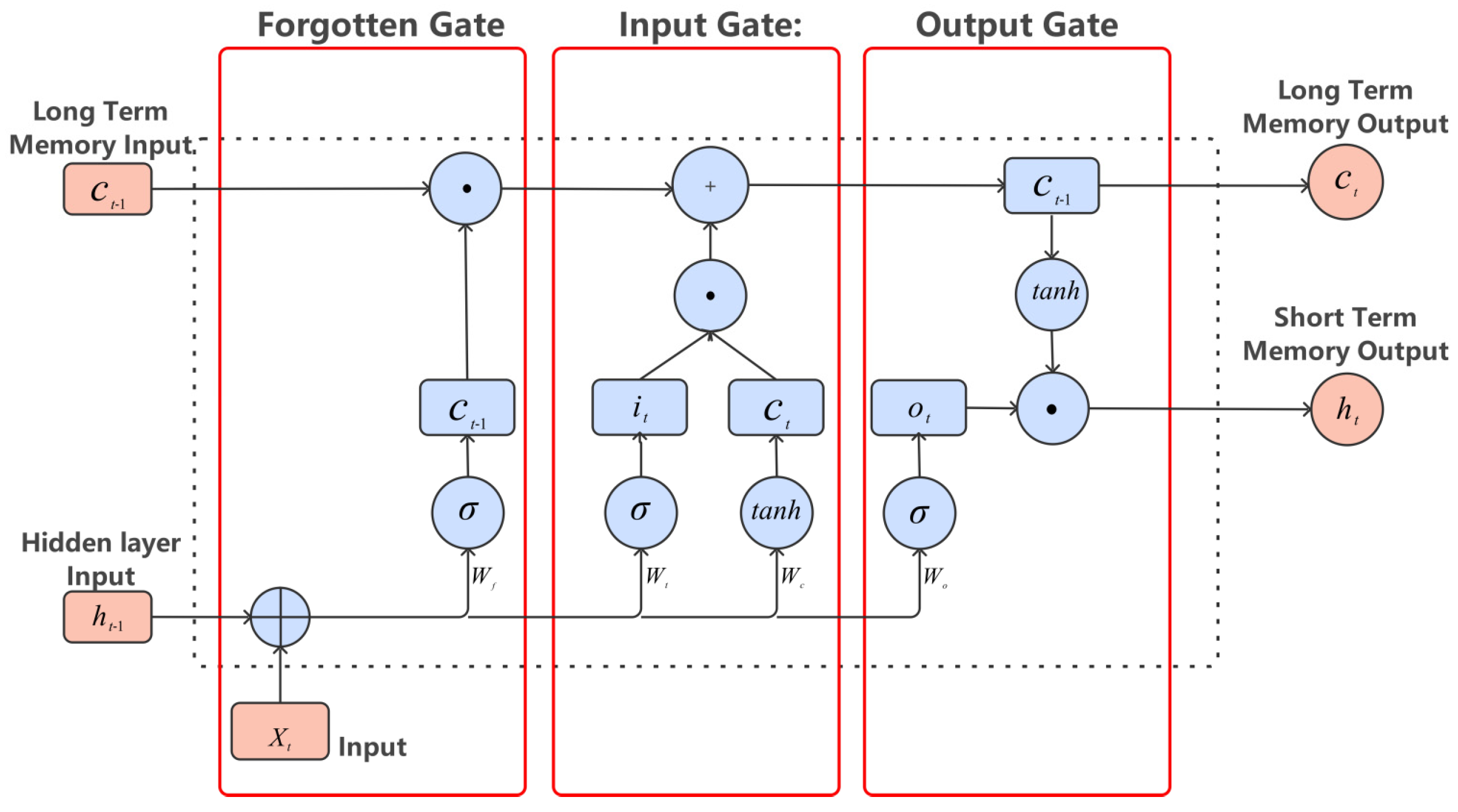
Figure 3. LSTM Time Series Flowchart.
Electronics 14 04475 g003

3.4. GWO-LSTM Prediction Model

LSTM neural networks, as a type of Recurrent Neural Network (RNN), effectively capture long-term dependencies in time series data due to their unique memory mechanism and gating structure. This makes them particularly well-suited for handling complex data with long-term memory characteristics. Consequently, LSTMs have been widely adopted in time series forecasting.
However, the performance of LSTM models heavily depends on the proper tuning of their network parameters (such as learning rate and number of hidden layer units). Traditional manual parameter tuning is time-consuming and struggles to find global optima, often resulting in suboptimal model performance. To address this, numerous intelligent optimization algorithms have emerged in recent years, such as genetic algorithms and particle swarm optimization. Gray Wolf Optimization (GWO), a novel intelligent optimization algorithm inspired by the social hierarchy and pack hunting strategies of gray wolves, possesses strong global search capabilities and convergence speed. It effectively optimizes LSTM hyperparameters, thereby enhancing the model’s prediction accuracy and generalization capability.
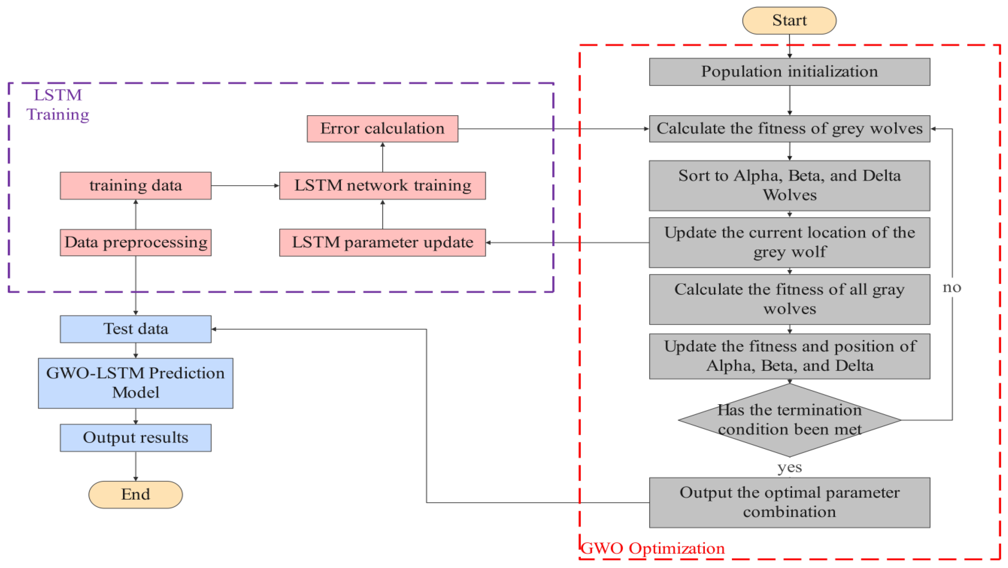
First, by integrating GWO with LSTM, we optimize LSTM model parameters to overcome the limitations of traditional manual tuning. LSTM performance relies on several critical parameters—including the number of hidden layer neurons, learning rate, and gradient clipping values—which directly impact training effectiveness and prediction accuracy. Manually adjusting these parameters is often time-consuming and labor-intensive, making it difficult to find optimal solutions. GWO, a global optimization algorithm based on swarm intelligence, efficiently searches multidimensional parameter spaces to identify the optimal parameter combinations for LSTMs. This approach enhances the model’s predictive accuracy and strengthens its generalization capabilities.
Second, this predictive model addresses the complexity and coupling of multiple variables within time series data. The nonlinearity, noise, periodicity, and multidimensionality of time series data pose significant challenges for traditional methods. LSTMs, however, offer distinct modeling advantages due to their ability to capture long-term dependencies. Integrating GWO further enhances LSTM capabilities, enabling more stable and high-precision predictions when handling complex, dynamic multivariate data. The overall model architecture comprises four major modules: data preprocessing, Gray Wolf Optimization, LSTM model construction and training, and prediction with visualization. Below is a detailed description of the architecture:
1.
Data Preprocessing Module: Performs standardization, missing value imputation, and outlier handling on input multivariate time series data to ensure data quality meets LSTM modeling requirements. Through data normalization, all input variables are transformed to the same scale, thereby eliminating model sensitivity to differences in variable scales.
2.
Gray Wolf Optimization Module (GWO): By simulating gray wolf hunting behavior and leveraging the characteristics of swarm intelligence, GWO performs global search and optimization of LSTM hyperparameters (such as learning rate, number of hidden layer units, etc.). GWO can rapidly identify optimal solutions across different parameter combinations, thereby enhancing the predictive performance of LSTM models. In the GWO-LSTM combined model, the fitness function f x is defined as:
f x = R M S E L S T M P V a l i d a t i o n   D a t a
In the formula, P = p 1 , p 2 , p 3 , p 4 , p 5 , where p 1 denotes the number of hidden layer neurons, p 2 represents the learning rate, p 3 indicates the number of hidden layer neurons, p 4 signifies the Dropout rate, and p 5 denotes the L2 regularization coefficient.
3.
LSTM Model Construction and Training Module: Utilize parameter configurations obtained through GWO optimization to build the LSTM model, establishing fundamental network structures such as input layers, hidden layers, and output layers. Employ the backpropagation algorithm for model training, implementing measures like gradient clipping to prevent gradient explosion or vanishing. The core components of an LSTM unit include the memory cell state and three gating structures. Its operational principle can be summarized as follows: the memory cell state C t 1 from the previous time step and the hidden layer state h t 1 are fed into the current time step unit. Combined with the current input sequence x t , these inputs undergo processing through the three gating structures to control information selection. This process calculates the current memory cell state C t and hidden layer state h t . Specifically: The forget gate f controls the degree of historical information decay in the memory cell; The input gate i determines how current input updates the memory cell state; The output gate o modulates the influence of the memory cell state on the current hidden state output. The formulas for calculating the forget gate f t , input gate i t , output gate o t , and candidate memory cell state C ~ t at time step t are as follows:
f t = sigmoid W f x t + U f h t 1 + b f i t = sigmoid W i x t + U i h t 1 + b i o t = sigmoid W o x t + U o h t 1 + b o C ~ t = tanh W C x t + U C h t 1 + b C
In the formula: W f , W i , W o , W C , U f , U i , U o , U C denote the weight matrices; b f , b i , b o , b C denote the biases.
4.
Prediction and Visualization Module: Utilizes trained models to generate predictions for test data. Visualizes the model’s predictive performance through charts such as actual-versus-predicted value comparisons and error distribution plots, enabling assessment of accuracy and stability.
The model flowchart is shown in Figure 4.

4. Case Study Analysis

4.1. Data Acquisition

This study utilizes operational data from the Qila Photovoltaic Power Station in Hotan Prefecture, Xinjiang, for the year 2019 as its foundational research sample. Data collection spans the complete annual cycle from early 2019 to early 2020, comprising photovoltaic output data recorded at 15 min intervals, totaling 35,040 datasets. Simultaneously acquired meteorological observation data originated from the National Meteorological Data Center, encompassing key parameters such as air temperature, module surface temperature, relative humidity, wind speed, total solar radiation, and atmospheric pressure. The raw observation data featured hourly temporal resolution. To address the temporal scale discrepancy between meteorological and power data, this study implemented a two-stage data processing strategy: First, missing values in meteorological records were imputed using the k-nearest neighbors algorithm. Subsequently, a multi-stage interpolation technique combining linear interpolation with cubic spline interpolation was applied to reconstruct the hourly meteorological data into a continuous dataset with 15 min granularity. After undergoing comprehensive data cleaning, normalization, and other preprocessing steps, the fused dataset was fed into machine learning models. The relationship diagram between the region’s climatic conditions and photovoltaic power generation data is shown in Figure 5.

4.2. Data Preprocessing

This study conducted feature analysis on the original photovoltaic operational dataset, revealing that the power plant’s effective generation period was concentrated between 07:30 and 19:30 local time [21]. To enhance modeling effectiveness, a time-period exclusion method was employed to remove data from nighttime periods where photovoltaic output was zero. After filtering, the effective sample size was reduced to 17,520 observation sets, strictly corresponding to the illumination period and maintaining synchronous alignment with meteorological data. Due to engineering factors such as inherent sensor biases and anomalies in photovoltaic array transmission circuits, the original dataset contained 12.6% outliers. Therefore, preprocessing and manual corrections were essential before utilizing the collected photovoltaic power generation data. This study employs linear interpolation method using SPSS Statistics 27 to effectively distinguish power fluctuations caused by equipment failures from those induced by cloud cover.

4.3. Pearson Correlation Coefficient Analysis

The Pearson correlation coefficient is a statistical measure of the linear relationship between two variables, denoted as r. Its values range from [−1, 1], and the specific calculation formula is as follows [22]:
r = x i x ¯ y i y ¯ ( x i x ¯ ) 2 ( y i y ¯ ) 2
where x i and y i are the observed values of the two variables, and x ¯ and y ¯ are the means of the two variables.
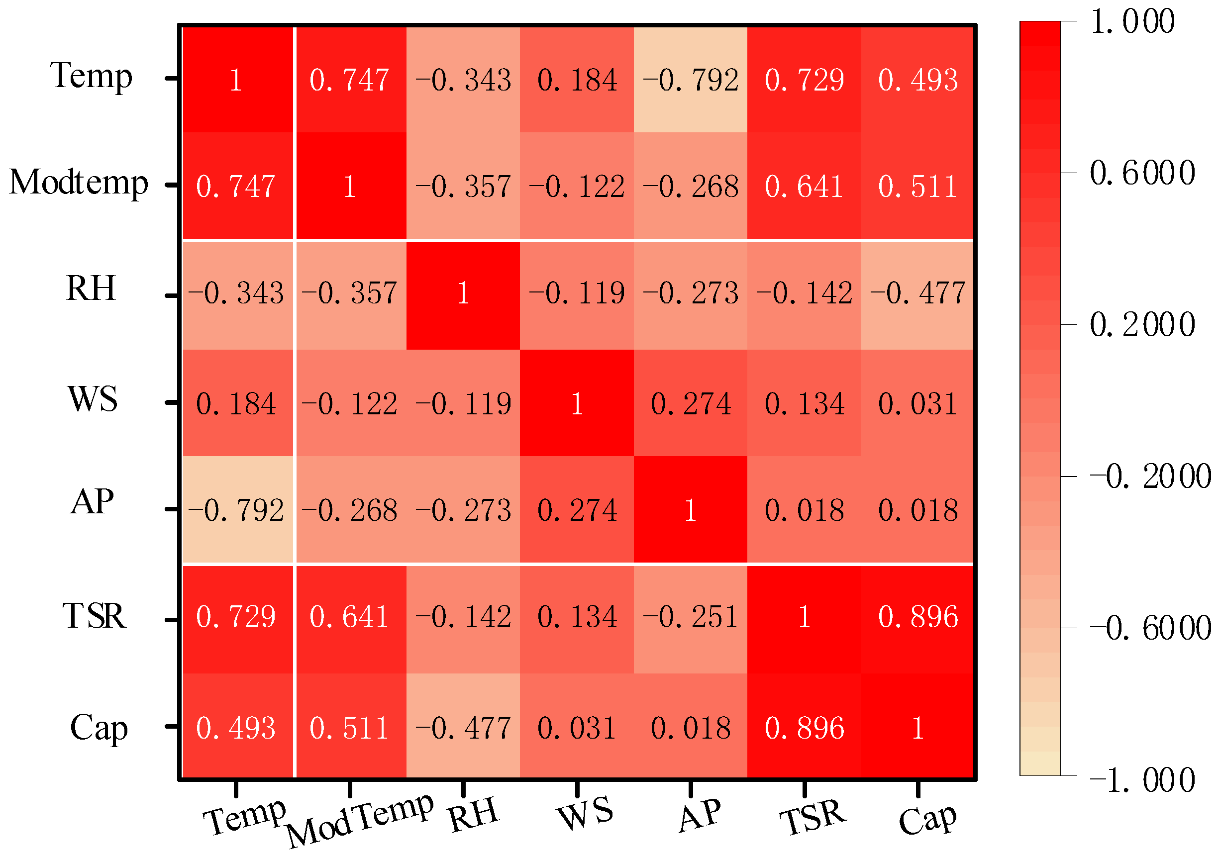
After preprocessing the data, historical photovoltaic power generation data and meteorological data were selected over a 20-day period with 15 min intervals. Meteorological factors included temperature (Temp), module surface temperature (ModTemp), humidity (RH), wind speed (WS), total solar radiation (TSR), and atmospheric pressure (AP). Data from periods of non-generation were excluded. Pearson correlation analysis was applied to the remaining data to calculate the correlation between meteorological factors and photovoltaic power generation [23]. The Pearson correlation coefficients between various meteorological factors and photovoltaic power generation (Cap) are presented in Figure 6.
As shown in Figure 6, air temperature, inter-module surface temperature, and total solar radiation exhibit positive correlations with PV power output, while humidity shows a negative correlation. Wind speed and atmospheric pressure demonstrate weak correlations with PV power output. Therefore, in establishing the GWO-LSTM model, air temperature, inter-module surface temperature, humidity, and total solar radiation are selected as input variables for the meteorological features in the prediction model.

4.4. K-Means Clustering Analysis

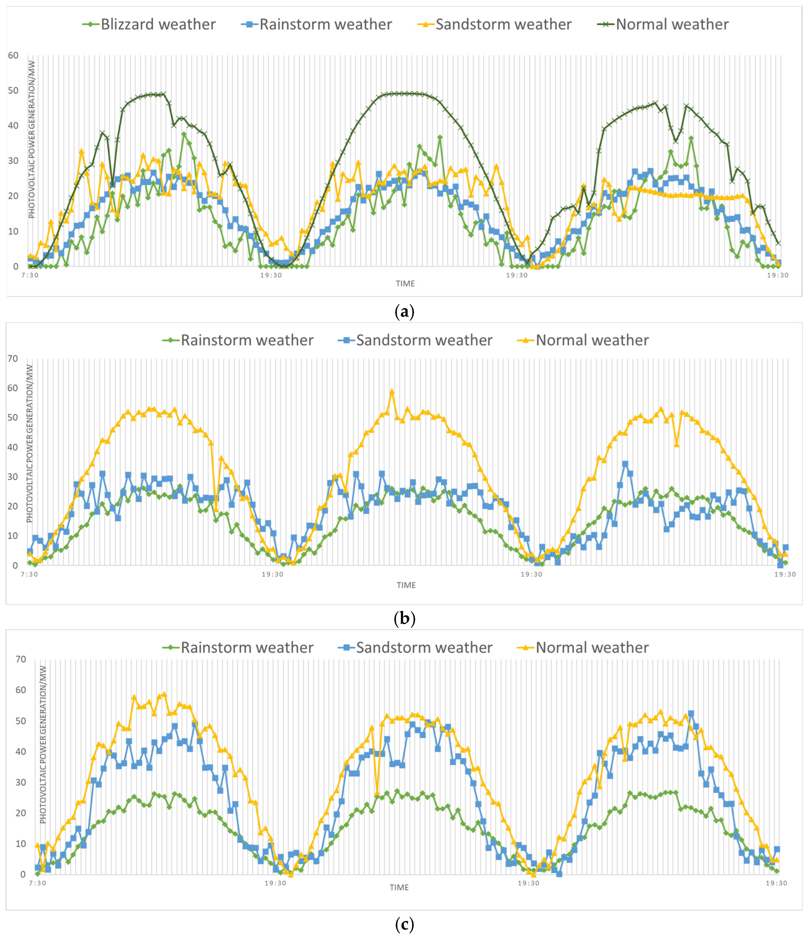
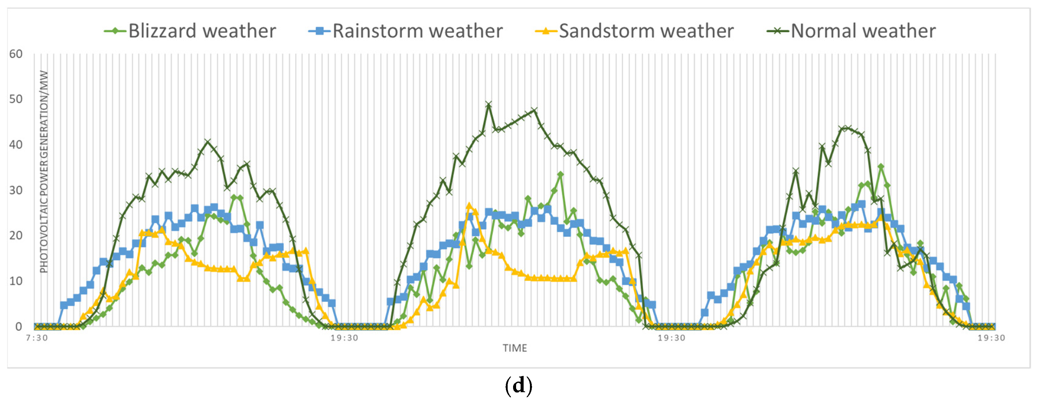
Based on photovoltaic power output analysis, a coupled classification system linking PV generation to meteorological modes is first established. The operational year is divided into four climatic subsets according to seasonal characteristics: spring (March–May), summer (June–August), autumn (September–November), and winter (December–February of the following year). Total irradiance, which best reflects PV power characteristics, is adopted as the feature parameter for cluster analysis. Input feature vectors for clustering include temperature, module surface temperature, humidity, wind speed, and atmospheric pressure. The elbow rule was applied to screen data for each season, setting the number of clusters k to 4: normal weather, heavy rain, heavy snow, and sandstorm conditions. After determining k = 4, clustering was performed for spring, summer, autumn, and winter. Clustering results are shown in Table 1.
After completing the clustering analysis of the annual climate, the classification results for the four seasons—spring, summer, autumn, and winter—were visualized separately. Figure 7 compares three randomly selected days of each weather type within the same season. The power generation curves for different weather types in the figure demonstrate that the clustering of the four weather types across the four seasons is effective. The distinct power generation characteristics under each weather type are clearly evident, facilitating the training of subsequent prediction models.

4.5. GWO-LSTM Prediction Experiments

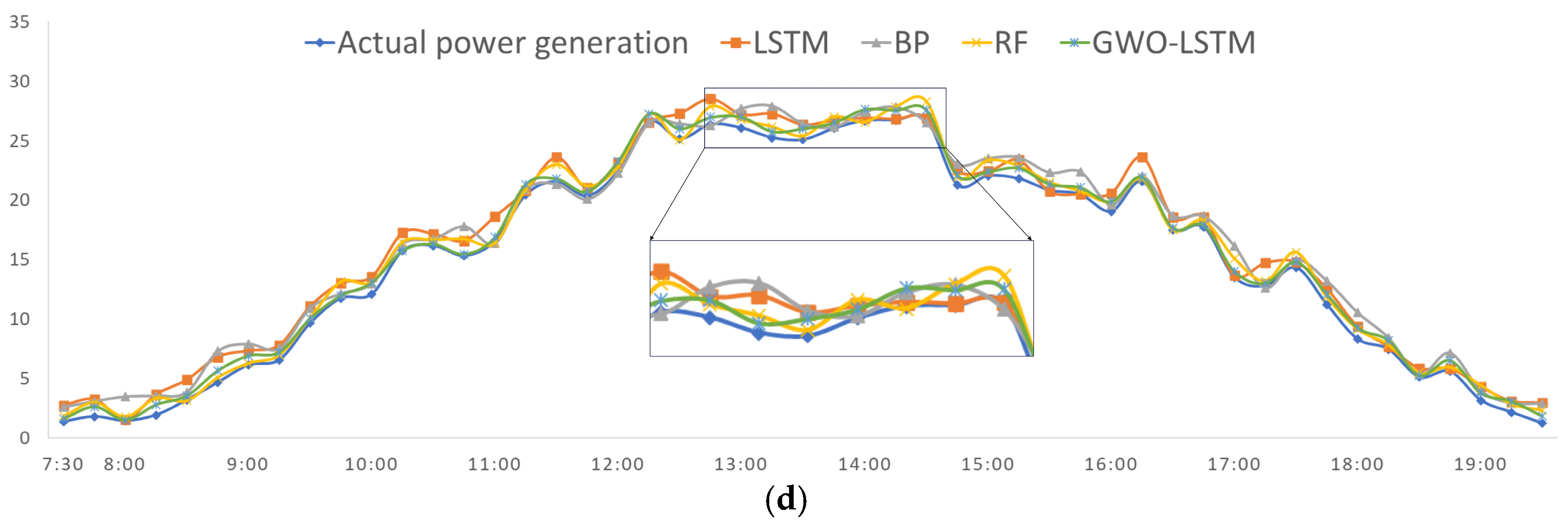
This paper proposes a GWO-LSTM photovoltaic power forecasting model based on K-means clustering to predict actual photovoltaic power output from 07:30 to 19:30 over the next day, with a 15 min sampling interval for the dataset. To validate the accuracy and superiority of the proposed model for short-term PV power forecasting, comparative experiments were conducted between the GWO-LSTM model and LSTM, BP, and RF prediction models. Test data were randomly sampled from the full dataset using a random function, comprising four days: 18 January (heavy snow), 20 February (sandstorm), 21 March (normal weather), and 17 September (heavy rain). The results are shown in Figure 8.
Figure 8 visually compares the prediction results of four models against actual measured PV power values for the test dataset. As seen on 21 March (normal weather), PV power exhibits minimal fluctuations under normal weather conditions. The basic BP and LSTM models perform poorly under this weather type, exhibiting not only significant errors relative to actual values but also considerable variability in predicted values. Test data from 18 January and 20 February reveal that during heavy rain or sandstorm weather, the Random Forest model performs relatively poorly. This is particularly evident at the beginning and middle sections of the curve, where deviations from actual measurements are substantial. This indicates that during extreme weather events like heavy rain or sandstorms, the RF prediction model is susceptible to the impact of drastic changes in climatic factors, leading to significant fluctuations and errors in prediction accuracy and precision. In contrast, the GWO-LSTM model, optimized using the GWO algorithm, demonstrates substantially improved prediction performance. For instance, in the test sets from 18 January and 20 February, the predicted values of the GWO-LSTM model closely align with the actual values, with the two curves nearly overlapping. For the 21 March test set, the prediction performance of the four models showed no significant difference. However, as shown in the local enlargement in Figure 8c, the GWO-LSTM model demonstrated superior prediction performance. Overall, the improved GWO-LSTM prediction model outperformed the pre-improvement LSTM, RF, and BP prediction models.
This paper employs Sum of Squares Error (SSE), Mean Absolute Error (MAE), Mean Squared Error (MSE), Root Mean Squared Error (RMSE), Mean Relative Error (MRE), and R-squared ( R 2 ) as performance metrics to evaluate the predictive capabilities of different forecasting models. Their specific calculation formulas are as follows:
E S S E = i = 1 N   x i x * i 2
E M A E = 1 N i = 1 N   x i x * i
E M S E = 1 N i = 1 N   ( x ( i ) x * ( i ) ) 2
E R M S E = 1 N i = 1 N   ( x ( i ) x * ( i ) ) 2
E M R E = 1 N i = 1 N   x i x * i x i
E R 2 = 1 i = 1 N   x i x * i i = 1 N   x i x ¯
In the equation, N is the sample size; x * i is the model prediction value; x i is the actual measured value; x ¯ is the sample mean.
As shown in Table 2, by calculating the SSE, MAE, MSE, RMSE, MRE and R 2 of photovoltaic forecast probabilities under normal weather, sandstorm weather, heavy rain weather, and heavy snow weather conditions using various prediction models, the following results are ultimately obtained.
The final average errors for BP, LSTM, RF, and GWO-LSTM across the four weather conditions are shown in Figure 9.
By calculating the SSE, MAE, MSE, RMSE, MRE and R 2 of various forecasting models for photovoltaic power prediction under different weather conditions, it can be observed that:
1.
Without using clustering algorithms, whether it is BP, LSTM, RF or GWO-LSTM, the prediction performance of the prediction model is not ideal, and the prediction error is relatively large. This is because the actual power generation is also influenced by climate factors in different seasons, and the daylight hours and photovoltaic intensity are different in different seasons of the year, which greatly interferes with the training effect of the model. The introduction of the clustering algorithm significantly reduces the error coefficient, indicating that training the prediction model separately with the four different weather data obtained through clustering can effectively improve the accuracy of the final prediction.
2.
In the case of snowstorms and rainstorms, the RMSE of RF is 0.20, −0.28, 0.49 and 0.43 lower than that of BP and LSTM, respectively, while in the case of normal weather, the RMSE of LSTM is 0.45 lower than that of RF, which indicates that the LSTM model performs better in more stable snowstorm data and performs worse than RF in rainstorm weather data with large fluctuations.
3.
The GWO-LSTM prediction model showed stable performance in all indicators in the prediction experiment of this article, and the prediction effect was relatively ideal. Compared with the basic prediction models of BP, LSTM, and RF, which have fluctuations in RMSE under four different weather types, the experimental results demonstrate the effectiveness of the GWO-LSTM combined model for photovoltaic power prediction, further verifying that the GWO-LSTM model has higher prediction accuracy in extreme weather conditions and can perform photovoltaic power prediction well in different weather types, thus verifying the reliability of this experimental method.
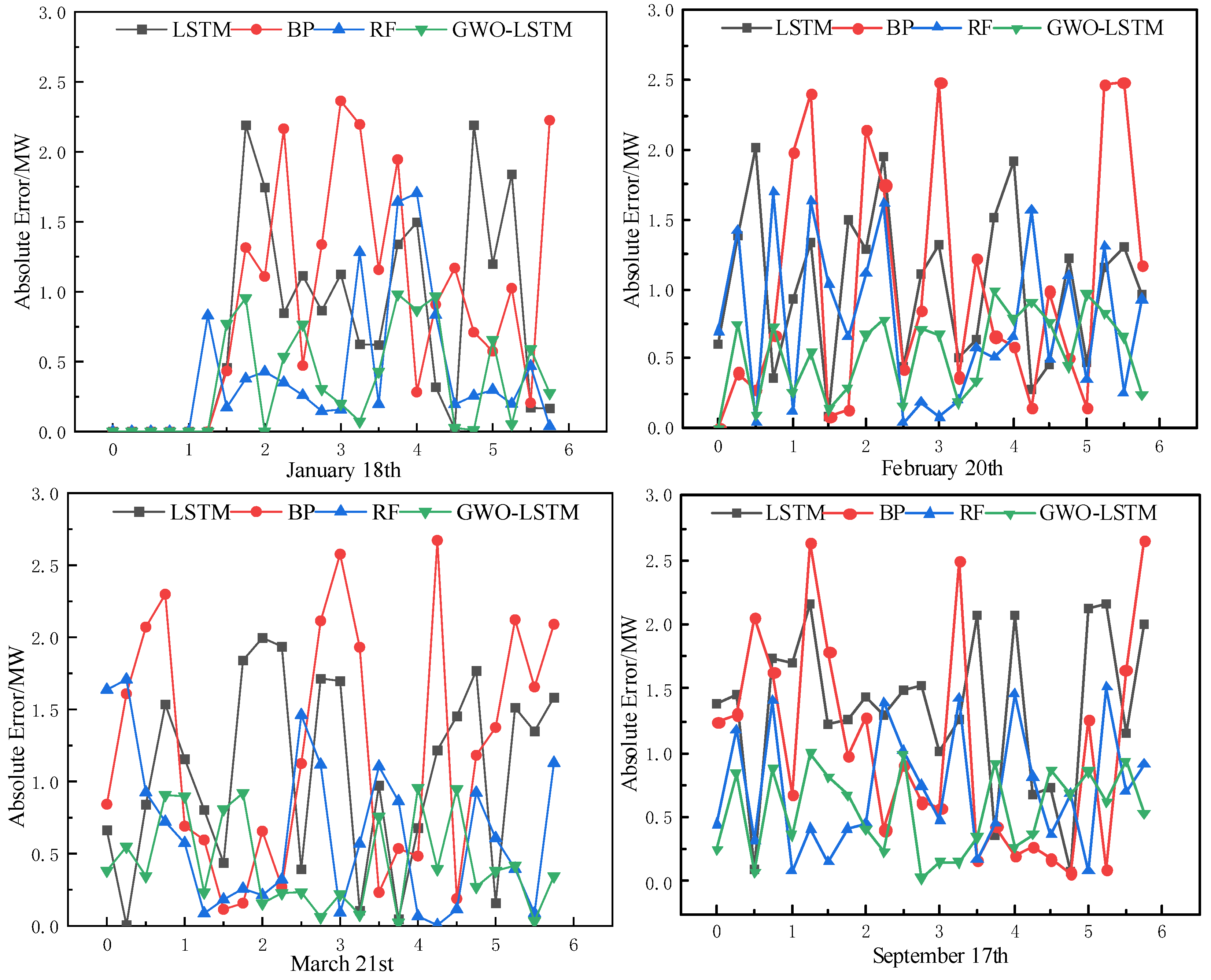
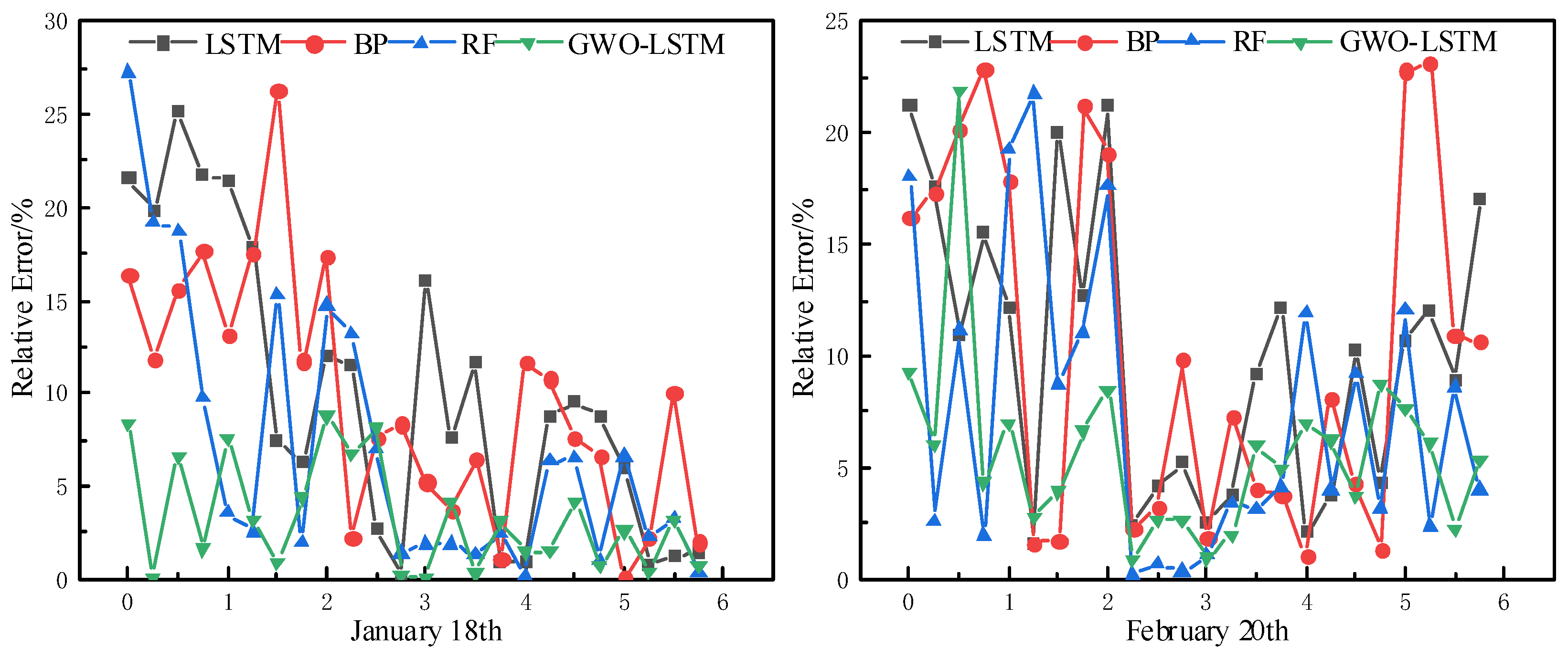
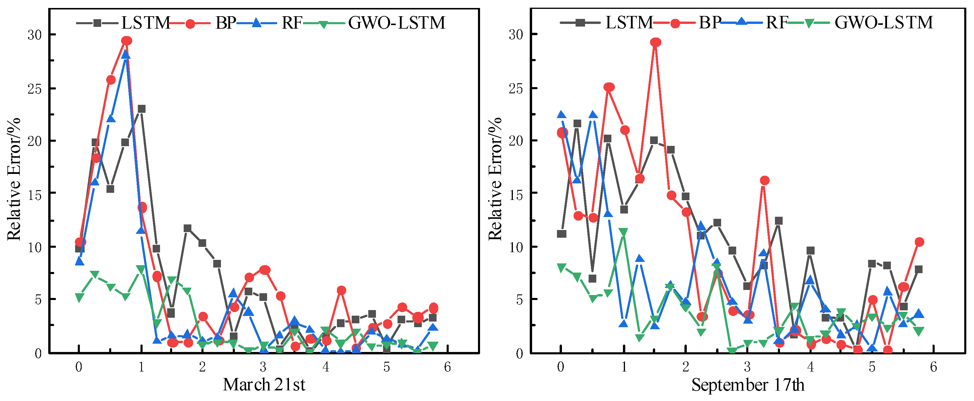
To further investigate whether the forecast results are stable, it is necessary to examine the prediction performance at individual points. Calculate the absolute error and relative error of each model at a single forecast point to observe the prediction accuracy at each point and the volatility of the overall forecast sequence. The formulas for absolute error E A and relative error E R are as follows:
E A = x i x * i × 100 %
E R = x i x * i x i × 100 %
The absolute errors and relative prediction errors for each point across the models in Figure 8 were calculated, with results shown in Figure 10 and Figure 11.
As shown in Figure 10, the BP prediction model performs poorly across all weather types after clustering, exhibiting significant fluctuations in absolute error with MAE = 0.8775. In contrast, LSTM and RF demonstrate relatively smaller fluctuations in absolute error compared to BP, though their error values remain substantial. Specifically, during the heavy rainfall event represented by 17 September, RF exhibited more stable absolute error compared to LSTM. Conversely, during the sandstorm event represented by 20 February, both LSTM and RF delivered suboptimal predictions, demonstrating susceptibility to environmental fluctuations associated with such weather conditions.
As shown in Figure 11, for the four weather types after clustering, the relative prediction errors for the 93.8% model points used in the experiment remained within 20%, while the GWO-LSTM model maintained relative prediction errors below 10% for nearly all prediction points. In terms of accuracy, the GWO-LSTM model demonstrated more precise single-point predictions compared to other forecasting models. Regarding stability, the relative prediction errors of single points across all models fluctuated to varying degrees over time. However, the GWO-LSTM model exhibited smaller fluctuations in prediction errors, indicating greater stability.

5. Conclusions

To address the uncertainty of photovoltaic power generation under extreme weather conditions, this paper proposes a K-means-based GWO-LSTM photovoltaic power generation short-term power prediction method. Through experiments and comparisons with other mainstream prediction models, the following conclusions were obtained:
  • After analyzing and preprocessing the data, Pearson correlation analysis and K-means clustering were used to classify the data into four categories based on weather conditions. Training separate prediction models for each weather type effectively improved the accuracy of the predictions.
  • The introduction of the gray wolf optimization algorithm to optimize the hyperparameters in the LSTM neural network automatically determines the optimal hyperparameters, avoiding the impact of hyperparameter setting errors on the experiment and further improving the prediction accuracy and model generalization capability.
  • Through comparative experimental analysis with other prediction models, it was verified that the GWO-LSTM model proposed in this paper can effectively improve the accuracy of photovoltaic power generation power prediction under extreme weather conditions, providing a new reference for predicting photovoltaic power generation power.

Author Contributions

Conceptualization, H.Z. and J.Z. (Jie Zheng); methodology, H.Z. and D.W.; formal analysis, H.Z. and F.X.; investigation, J.Z. (Jizhong Zhu); resources, W.Z.; writing—original draft preparation, J.Z. (Jie Zheng); writing—review and editing, J.Z. (Jizhong Zhu). All authors have read and agreed to the published version of the manuscript.

Funding

This work is supported by the Southern Power Grid Corporation Science and Technology Project (030700KC23120031(GDKJXM20231388)).

Data Availability Statement

The datasets presented in this paper are not readily available because the data belongs to the ongoing Southern Power Grid Corporation Science and Technology Project. Requests to access the datasets should be directed to the corresponding author.

Conflicts of Interest

Authors Haomin Zhang, Daoyuan Wang, Fei Xue and Wei Zou were employed by Jiangmen Power Supply Bureau, Guangdong Power Grid Co., Ltd. Jizhong Zhu were employed South China University of Technology. All authors declare that the research was conducted in the absence of any commercial or financial relationships that could be construed as a potential conflict of interest.

References

  1. Wang, L.; Li, C.; Liu, J.; Li, C. Short Term Photovoltaic Power Prediction Based on GRO-SSA-LSTM. J. Sol. Energy 2025, 46, 401–409. [Google Scholar] [CrossRef]
  2. Wang, S.; Li, H.; Ma, G.; Yuan, Y.; Bu, Q.; Ye, Z. Multistep Prediction Model for Photovoltaic Power Generation Based on Time Convolution and DLinear. Power Constr. 2025, 46, 173–184. [Google Scholar]
  3. Peng, S.; Chen, H.; Sun, W. Research on Photovoltaic Power Prediction Method Based on Improved LSTM. J. Sol. Energy 2024, 45, 296–302. [Google Scholar] [CrossRef]
  4. Wang, D.; An, Y.; Liao, C. Research on Photovoltaic Power Generation Prediction Method Based on CNN-LSTM Hybrid Neural Network. J. Xi’an Pet. Univ. (Nat. Sci. Ed.) 2024, 39, 129–134. [Google Scholar]
  5. Liu, Y.; Chen, Y. Short-Term Photovoltaic Power Forecasting Based on RF Feature Extraction and TCN-BiGRU Model. Chin. J. Sol. Energy 2025, 46, 682–689. [Google Scholar] [CrossRef]
  6. Liu, D.; Wang, W.; Zhang, H.; Li, G.; Xiao, G.; Zhang, B. Application of Medium- and Long-Term Electricity Forecasting and Dispatch Planning for Photovoltaic Power Based on Hidden Markov Model Correction. High Volt. Eng. 2023, 49, 840–848. [Google Scholar] [CrossRef]
  7. Wang, R.; Gao, Q.; Lu, J. Short-Term Photovoltaic Power Forecasting Based on the CEEMDAN-LSSVM-ARIMA Model. Sens. Microsyst. 2022, 41, 118–122. [Google Scholar] [CrossRef]
  8. Wu, Y.; Rong, W.; Guo, Y.; Ye, J. Short-Term Photovoltaic Power Forecasting Based on SVMD-IDBO-KELM. Chin. J. Sol. Energy 2025, 46, 271–279. [Google Scholar] [CrossRef]
  9. Chen, S.; Jiang, J.; Li, S. Review of Power Prediction Methods for Photovoltaic Systems Under Extreme Weather Conditions. Trans. Chin. Soc. Electr. Eng. 2025, 20, 281–290. [Google Scholar]
  10. Ye, L.; Pei, M.; Lu, P.; Zhao, J.; He, B. Short-Term Photovoltaic Power Combination Forecasting Method Based on Weather Sub-Types. Autom. Electr. Power Syst. 2021, 45, 44–54. [Google Scholar]
  11. Dong, B. Analysis of Distributed Photovoltaic Metering Power Prediction and Optimization. Electron. Technol. 2025, 54, 302–303. [Google Scholar]
  12. Lorenz, E.; Heinemann, D.; Kurz, C. Local and regional photovoltaic power prediction for large scale grid integration: Assessment of a new algorithm for snow detection. Prog. Photovolt. Res. Appl. 2012, 20, 760–769. [Google Scholar] [CrossRef]
  13. Levent, İ.; Şahin, G.; Işık, G.; van Sark, W.G. Comparative Analysis of Advanced Machine Learning Regression Models with Advanced Artificial Intelligence Techniques to Predict Rooftop PV Solar Power Plant Efficiency Using Indoor Solar Panel Parameters. Appl. Sci. 2025, 15, 3320. [Google Scholar] [CrossRef]
  14. Liu, J.; Fang, W.; Zhang, X.; Yang, C. An Improved Photovoltaic Power Forecasting Model With the Assistance of Aerosol Index Data. IEEE Trans. Sustain. Energy 2015, 6, 434–442. [Google Scholar] [CrossRef]
  15. Raman, R.; Mewada, B.; Meenakshi, R.; Jayaseelan, G.M.; Sharmila, K.S.; Taqui, S.N.; Al-Ammar, E.A.; Wabaidur, S.M.; Iqbal, A. Forecasting the PV power utilizing a combined convolutional neural network and long short-term memory model. Electr. Power Compon. Syst. 2024, 52, 233–249. [Google Scholar] [CrossRef]
  16. Chen, J.; Yang, J.; Zhai, Y.; Li, B.; Zeng, Q. Prediction of Ash Accumulation Degree of Photovoltaic Modules Based on Average Grayscale Value and Random Forest Algorithm. J. Sol. Energy 2024, 45, 107–114. [Google Scholar] [CrossRef]
  17. Jiang, M.; Ding, K.; Chen, X.; Cui, L.; Zhang, J.; Yang, Z.; Cang, Y.; Cao, S. Research on time-series based and similarity search based methods for PV power prediction. Energy Convers. Manag. 2024, 308, 118391. [Google Scholar] [CrossRef]
  18. Huang, M.; Xing, F.; Chen, X.; Lu, M. Short-Term Photovoltaic Power Forecasting Based on a Combined Al-gorithm of K-Means Clustering and Extreme Learning Machine. Hydro Power Energy Sci. 2024, 42, 217–220+216. [Google Scholar] [CrossRef]
  19. Mirjalili, S.; Mirjalili, S.M.; Lewis, A. Grey wolf optimizer. Adv. Eng. Softw. 2014, 69, 46–61. [Google Scholar] [CrossRef]
  20. Duan, B.; Ma, Y.; Liu, J.; Jin, Y. Nonlinear Grey Wolf Optimization Algorithm based on Chaotic Mapping and Reverse Learning Mechanism. Softw. Eng. 2023, 26, 36–40. [Google Scholar] [CrossRef]
  21. Li, C.; Yang, Y.; Song, J.; Zhang, X.; Xu, Q. Short Term Photovoltaic Power Generation Prediction based on IMVMD and BILSTM-SARIMA Combination Model in Station Area. J. Sol. Energy 2025, 46, 433–440. [Google Scholar] [CrossRef]
  22. Li, X.; Cao, L.; Li, Z.; Li, J.; Lv, X. Influence of Leakage from Buried Drainage Pipes on Shallow Soil Settlement and Urban Road Collapse. Nat. Hazards Rev. 2025, 26, 04025017. [Google Scholar] [CrossRef]
  23. Shi, H.; Guo, L.; Liu, Y.; Wang, C. Short-term forecasting of photovoltaic power based on total irradiance correction of multi-source meteorological forecast. Electr. Power Autom. Equip. 2022, 42, 104–112. [Google Scholar] [CrossRef]
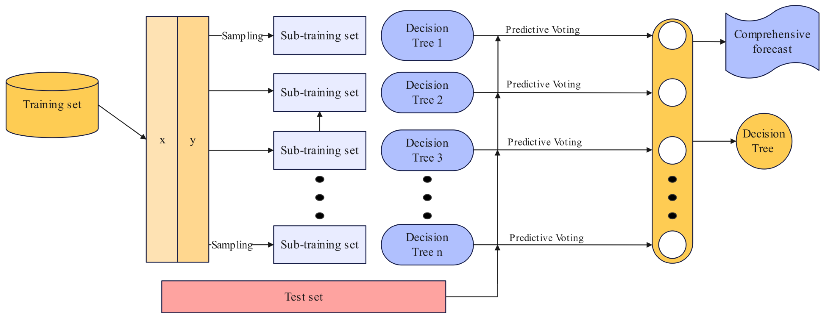
Figure 1. Random Forest Model Flowchart.
Electronics 14 04475 g001
Figure 2. Gray Wolf Position Diagram.
Electronics 14 04475 g002
Figure 4. GWO-LSTM Flowchart.
Electronics 14 04475 g004
Figure 5. Relationship Diagram Between Climate Conditions and Photovoltaic Power Generation Data.
Electronics 14 04475 g005
Figure 6. Pearson Correlation Coefficient Between Meteorological Factors and Photovoltaic Power Output.
Electronics 14 04475 g006
Figure 7. Four seasons K-means clustering results. (a) Spring. (b) Summer. (c) Autumn. (d) Winter.
Electronics 14 04475 g007aElectronics 14 04475 g007b
Figure 8. Comparison of prediction results from four models and actual power measurements. (a) 18 January. (b) 20 February. (c) 21 March. (d) 17 September.
Electronics 14 04475 g008aElectronics 14 04475 g008b
Figure 9. Average error for each prediction model under four weather conditions.
Electronics 14 04475 g009
Figure 10. Absolute Error at Each Forecast Point Under Various Weather Conditions.
Electronics 14 04475 g010
Figure 11. Relative Error at Each Forecast Point Under Various Weather Conditions.
Electronics 14 04475 g011aElectronics 14 04475 g011b
Table 1. K-means Clustering Analysis Results Table.
SeasonWeather TypeNumber of DaysSeasonWeather TypeNumber of Days
SpringNormal weather90AutumnNormal weather92
Rainstorm weather13 Rainstorm weather15
Snowstorm weather7 Snowstorm weather0
Sandstorm weather18 Sandstorm weather24
SummerNormal weather91WinterNormal weather92
Rainstorm weather3 Rainstorm weather14
Snowstorm weather0 Snowstorm weather14
Sandstorm weather31 Sandstorm weather17
Table 2. SSE, MAE, MSE, RMSE, MRE and R 2 of Various Models under Different Weather Types.
Weather TypeModel NameSSEMAEMSERMSEMRE R 2
Normal weatherBP118.5741.3022.4191.5551.9240.915
LSTM81.9510.6880.7630.8730.1320.926
RF37.4181.1371.6721.2931.9540.955
GWO-LSTM14.8450.4650.3020.5500.1500.970
Snowstorm weatherBP80.5270.9721.6431.2810.7060.875
LSTM57.2190.5430.6250.7910.8510.897
RF30.6730.7971.1671.0810.3090.930
GWO-LSTM14.8260.4130.3020.5500.2670.947
Rainstorm weatherBP87.8701.1121.7931.3390.1990.853
LSTM80.2551.0941.6371.2790.1800.856
RF35.7290.7240.7290.8530.1120.904
GWO-LSTM21.6570.5930.4410.6640.0870.922
Sandstorm weatherBP69.1300.4910.5070.7120.1640.861
LSTM44.5510.7280.9090.9530.2430.881
RF24.8790.85311.4101.1870.1780.920
GWO-LSTM14.3560.4220.2920.5410.1230.931
Unclustered weatherBP94.1452.8713.2181.7941.6290.826
LSTM103.8372.4892.9811.7260.8920.815
RF59.1982.2122.4361.5600.4150.880
GWO-LSTM37.0281.9182.1891.4790.3190.893
Disclaimer/Publisher’s Note: The statements, opinions and data contained in all publications are solely those of the individual author(s) and contributor(s) and not of MDPI and/or the editor(s). MDPI and/or the editor(s) disclaim responsibility for any injury to people or property resulting from any ideas, methods, instructions or products referred to in the content.