HRformer: A Hybrid Relational Transformer for Stock Time Series Forecasting

Abstract

Stock trend prediction is a complex and crucial task due to the dynamic and nonlinear nature of stock price movements. Traditional models struggle to capture the non-stationary and volatile characteristics of financial time series. To address this challenge, we propose the Hybrid Relational Transformer (HRformer), which specifically decomposes time series into multiple components, enabling more accurate modeling of both short-term and long-term dependencies in stock data. The HRformer mainly comprises three key modules: the Multi-Component Decomposition Layer, the Component-wise Temporal Encoder (CTE), and the Inter-Stock Correlation Attention (ISCA). Our approach first employs the Multi-Component Decomposition Layer to decompose the stock sequence into trend, cyclic, and volatility components, each of which is independently modeled by the CTE to capture distinct temporal dynamics. These component representations are then adaptively integrated through the Adaptive Multi-Component Integration (AMCI) mechanism, which dynamically fuses their information. The fused output is subsequently refined by the ISCA module to incorporate inter-stock correlations, leading to more accurate and robust predictions. Extensive experiments on the NASDAQ100 and CSI300 datasets demonstrate that HRformer consistently outperforms state-of-the-art methods, e.g., achieving about 0.83% higher Accuracy and 1.78% higher F1-score than TDformer on NASDAQ100, with Sharpe Ratios of 1.5354 on NASDAQ100 and 0.5398 on CSI300, especially in volatile market conditions. Backtesting results validate its practical utility in real-world trading scenarios, showing its potential to enhance investment decisions and portfolio performance.

1. Introduction

The rapid development of the stock market has created an attractive yet risky environment, drawing numerous investors and traders seeking to maximize profits. Stock trend prediction, which aims to forecast future stock price movements to support investment decisions, has become a significant research topic [1,2,3]. However, accurately predicting stock trends remains a challenging task due to the highly volatile and non-stationary characteristics of the financial market.

Stock trend prediction can be formulated as a time series forecasting problem [4,5,6]. Traditional approaches mainly rely on statistical models, such as ARIMA [7] and VAR [8], to analyze stock volatility based on indicators like daily closing prices. However, stock price series typically exhibit nonlinear and dynamic behavior. Compared with statistical models, machine learning methods are more capable of capturing nonlinear relationships in time series data. Various machine learning algorithms, including SVM [9], RVFL [10], and Random Forest [11], have been applied to stock prediction tasks [11,12], demonstrating moderate success [13]. Nevertheless, these traditional models often depend heavily on manual feature engineering and domain expertise to describe complex stock movements. They also struggle to capture high-order nonlinear dependencies among stocks, resulting in reduced prediction performance under volatile market conditions.

In recent years, deep learning techniques have shown strong potential in uncovering latent market dynamics, especially in modeling stock prices and movement trends [14,15,16]. Existing deep learning-based methods usually focus on either local temporal variations or long-term dependencies. Recurrent neural network (RNN)-based architectures, such as Long Short-Term Memory (LSTM) networks [17,18] and Gated Recurrent Units (GRUs) [19], can accurately capture short-term temporal dependencies in stock sequences. Temporal Convolutional Networks (TCNs) [20,21] offer high parallelism and long-range dependency modeling, making them competitive alternatives. Transformer-based models such as Informer [22], FEDformer [23], TDformer [24], and iTransformer [25] further excel at capturing long-term dependencies, with FEDformer leveraging frequency decomposition, TDformer fusing temporal-frequency attention, and iTransformer adopting inverted attention for efficient multivariate forecasting. However, these methods often overlook the inherent non-stationary and fluctuating properties of financial time series, which limits their ability to represent dynamic and chaotic stock behaviors accurately. In contrast, decomposition-based models have shown improved robustness in modeling complex patterns, as they can extract both global and local temporal structures more effectively. For instance, Autoformer [26] employs a decomposition mechanism with Auto-Correlation to improve long-term forecasting, and FEDformer [23] integrates frequency–domain decomposition with Transformer-based architectures to enhance both global and local dependency modeling. Beyond temporal modeling, recent research has emphasized the importance of spatial–temporal correlations in stock data. For example, Wang et al. proposed a Localized Graph Convolutional Network (LoGCN) [21] that effectively captures spatial-temporal dependencies using localized graph convolution.

Despite these advancements, accurately forecasting stock prices in real-world settings remains highly challenging. Existing models still face difficulties in addressing non-stationary fluctuations and capturing dynamic relationships inherent in chaotic market behaviors. Several key challenges persist:

• Complex Temporal Patterns in Stock Data: Stock price movements are influenced by various internal temporal dynamics, including trend, cyclic, and volatility. These components exhibit distinct time dependencies, with trend capturing long-term movements, cyclic modeling periodic patterns, and volatility representing short-term irregular fluctuations. However, many existing methods fail to effectively extract all three types of temporal relationships, especially the time-varying nature of short-term volatility and its interaction with long-term trends and cycles. To enhance prediction performance, it is essential to model these temporal dependencies and their dynamic interactions over time.
• Inter-Stock Correlation Modeling: Stock price movements are often interdependent, with the behavior of one stock influencing others. Accurately capturing these cross-stock dependencies is essential for improving forecasting performance. Many existing methods inadequately model these inter-stock correlations, leading to incomplete representations of the market’s relational structure. By focusing on inter-stock correlation modeling, we can better understand the complex relationships between stocks and improve predictive accuracy across different market conditions.

Motivated by these challenges, we propose an end-to-end framework named the Hybrid Relational Transformer (HRformer) for stock trend prediction. The HRformer framework is composed of three main components: the Multi-Component Decomposition Layer, the Component-wise Temporal Encoder (CTE) with an Adaptive Multi-Component Integration (AMCI) module, and the Inter-Stock Correlation Attention (ISCA) mechanism.

First, the Multi-Component Decomposition Layer decomposes each stock time series into three distinct components: trend, cyclic, and volatility. The trend component captures the overall long-term direction of stock movements, the cyclic component represents periodic behaviors occurring at different frequencies (such as daily or weekly cycles), and the volatility component models irregular short-term fluctuations that cannot be explained by the other two components. This decomposition allows the model to better capture the complex temporal relationships within each stock (intra-stock temporal dependencies). Second, the CTE models each component separately to capture its specific temporal dynamics. The trend component is processed by a Transformer encoder to capture long-term dependencies, the cyclic component is modeled using frequency-enhanced attention to capture periodic signals, and the volatility component is handled using normalization (RevIN), a multilayer perceptron (MLP), and a recurrent unit (LSTM) to represent nonlinear short-term dynamics. This enables the model to model the complex temporal dependencies within each component (intra-stock dependencies). The AMCI module dynamically fuses the learned component representations through adaptive gating weights, allowing the model to adjust the contribution of each component over time. Finally, the ISCA mechanism models the inter-stock correlations by capturing dependencies among multiple stocks through multi-head attention, learning the inter-stock relationships and co-movements in the market.

By integrating both intra-stock temporal modeling and inter-stock correlation learning, HRformer can robustly capture the rich and diverse dependencies in stock time series, improving forecasting accuracy across various market conditions. We evaluate the HRformer on two benchmark datasets, NASDAQ100 and CSI300, and compare it with various baseline models. Experimental results demonstrate that HRformer consistently outperforms state-of-the-art forecasting approaches, especially under volatile market conditions. Backtesting and ablation studies further verify the robustness and interpretability of each module and confirm the practical value of the proposed framework in real-world trading scenarios.

The main contributions of this study are summarized as follows:

• We propose the HRformer, which jointly models intra-stock temporal dynamics and inter-stock correlations. The Multi-Component Decomposition Layer extracts trend, cyclic, and volatility components from each stock series, while the Adaptive Multi-Component Integration (AMCI) module dynamically balances their contributions. To capture cross-stock relationships, the Inter-Stock Correlation Attention (ISCA) applies multi-head attention to learn dependencies and market co-movements. By unifying component-wise modeling and correlation learning, HRformer effectively captures complex dependencies in stock time series and enhances forecasting performance across market conditions.
• The Component-wise Temporal Encoder (CTE) models intra-stock dynamics by processing trend, cyclic, and volatility components separately: a Transformer encoder captures long-term trends, frequency-enhanced attention models periodic patterns, and a RevIN–MLP–LSTM structure represents short-term fluctuations. The Adaptive Multi-Component Integration (AMCI) module then fuses these representations, while the Inter-Stock Correlation Attention (ISCA) captures cross-stock dependencies and market co-movements, forming a unified temporal–spatial representation.
• Comprehensive experiments and backtesting confirm that HRformer achieves superior predictive performance and practical robustness compared with representative stock forecasting models, while ablation studies validate the contribution of each module.

The remainder of this paper is organized as follows. Section 2 reviews related work, and Section 3 introduces the problem formulation. Section 4 presents the detailed architecture of the proposed HRformer framework, while Section 5 reports experimental evaluations. Section 6 provides an analysis of the results, and Section 7 concludes the study with insights and future research directions.

2. Related Work

2.1. Deep Learning Based Stock Trend Prediction

With the rapid advancement of deep learning, numerous models have been developed for analyzing and forecasting time series data. Recurrent Neural Networks (RNNs) have demonstrated strong capabilities in capturing short-term temporal dependencies due to their sequential processing nature. For instance, Long Short-Term Memory (LSTM) networks have been applied to short-term traffic flow forecasting tasks [27], while DeepAR, an auto-regressive recurrent model, has shown effectiveness in probabilistic forecasting across diverse time series scenarios, achieving robust performance in capturing temporal patterns and dependencies [28].

More recently, Transformer-based architectures have achieved competitive performance in long-term time series forecasting. The self-attention mechanism of Transformers [29] allows for efficient modeling of long-range dependencies and global information extraction. For example, the Informer model [22] introduces a ProbSparse self-attention mechanism that enhances scalability and efficiency for long sequence forecasting. Similarly, Crossformer [30] explicitly models both cross-time and cross-variable dependencies, improving its capability to represent multivariate temporal relationships. Models such as PatchTST [31] and iTransformer [25] further extend the Transformer framework by applying attention across transposed dimensions, allowing for improved feature extraction and dependency modeling in multivariate time series.

In the context of stock trend prediction, RNN-based and Transformer-based architectures have been widely adopted to model temporal behaviors in stock data. LSTM-based approaches have been particularly successful due to their ability to learn temporal dependencies from sequential financial data. For example, Li et al. [32] proposed a multimodal event-driven LSTM that integrates market fundamentals and news information to enhance prediction accuracy. Zeng et al. [33] combined CNN and Transformer architectures to jointly capture short-term and long-term dependencies in financial time series, achieving competitive results in intraday stock forecasting.

However, these models still face significant challenges when applied to real-world financial forecasting. Traditional deep learning architectures often struggle with the non-stationarity and high volatility of stock prices, resulting in unstable performance. Furthermore, many existing approaches fail to effectively incorporate decomposition-based structures that can separate trend, cyclic, and volatility behaviors—key aspects for accurately modeling complex financial dynamics. To address these issues, this paper introduces a decomposition-driven approach that explicitly models different temporal components and dynamically integrates them, providing a more adaptive and robust solution for stock trend forecasting.

2.2. Decomposition-Based Time Series Forecasting Methods

Decomposition methods have gained significant attention in time series forecasting due to their ability to decompose complex signals into interpretable subcomponents [34,35]. These methods enable the isolation of distinct temporal patterns, such as trends and periodic variations (e.g., STL decomposition [36]), which are often difficult to identify directly in raw data. Many recent studies have integrated decomposition strategies to enhance the predictive capacity of deep learning architectures.

TimesNet [37] decomposes complex variations across multiple periods and jointly models intra-period and inter-period dependencies by transforming one-dimensional time series into a two-dimensional representation. Autoformer [26] employs a decomposition structure to separate time series into trend and seasonal components, using an Auto-Correlation mechanism to better capture long-term dependencies. DLinear [38] performs a simple moving average decomposition and models the trend and seasonal components through multilayer perceptrons (MLPs). FEDformer [23] integrates frequency-enhanced decomposition with Transformer-based architectures, combining seasonal–trend separation and global–local dependency modeling to improve forecasting accuracy. N-BEATS [39] models trend using low-degree polynomials and represents seasonality with Fourier series, while N-HiTS [40] extends this framework through multi-rate sampling to capture multi-scale temporal variations.

Although these approaches effectively improve interpretability and performance in general time series forecasting, their direct application to stock trend prediction remains limited. The financial market’s high volatility and multi-periodic behaviors introduce complexities that standard decomposition techniques struggle to capture. Our proposed Hybrid Relational Transformer (HRformer) extends this line of research by employing a Multi-Component Decomposition Layer that extracts trend, cyclic, and volatility components through both time–domain smoothing and frequency–domain filtering. In addition, the framework incorporates a Component-wise Temporal Encoder (CTE) and an Adaptive Multi-Component Integration (AMCI) module to dynamically combine learned representations, addressing the non-stationary and multi-scale nature of stock data. This design enables HRformer to more effectively model multi-periodicity, cross-variable dependencies, and non-linear fluctuations, achieving improved robustness and accuracy in financial forecasting.

2.3. Fusion Methods in Time Series Forecasting

Fusion strategies have emerged as an effective means to enhance the predictive capability of time series models, particularly when the data exhibit complex structures or multiple temporal components. These approaches combine multiple representations, models, or features to exploit complementary information and improve forecasting performance. For instance, H-MMoE [41] improves multi-task learning by fusing multimodal data. Similarly, Tang et al. [42] combine ARIMA and neural network models through empirical mode decomposition (EMD) and hybrid fusion to enhance prediction accuracy in chaotic time series.

TDformer [24] employs a simple additive fusion strategy to combine decomposed trend and seasonal components, where individual outputs are summed to obtain the final forecast. Although computationally efficient, this approach cannot fully capture the complex interdependencies among temporal components. The PDF model [43] advances this concept by introducing a Variations Aggregation Block, which separately models short- and long-term variations before combining them through shared linear transformations to balance contributions across multiple components.

Building upon these ideas, our proposed HRformer introduces an Adaptive Multi-Component Integration (AMCI) module that dynamically fuses the trend, cyclic, and volatility representations learned from the Multi-Component Decomposition Layer. This adaptive gating design allows the model to flexibly adjust the weight of each component according to its relevance at each time step. The resulting integrated representation is further refined through the Inter-Stock Correlation Attention (ISCA) mechanism, which captures spatial dependencies among different stocks. This adaptive and hierarchical fusion strategy enables HRformer to achieve greater robustness and accuracy in forecasting highly volatile and non-stationary financial time series.

3. Problem Formulation

To support stock selection and maximize investment returns, we formulate stock trend prediction as a binary classification task that aims to determine whether each stock will rise or fall in the next trading period. Accurate prediction of stock movements is crucial, as it can significantly enhance portfolio performance and risk control.

Let $\mathbf{S}=\{s_1,\dots ,s_M\}$ denote a set of M stocks. For each stock $s_i\in \mathbf{S}$, we collect a sequence of technical indicators on each trading day t, such as opening price, closing price, highest price, and lowest price. The historical sequence data of each stock is represented as ${\mathbf{x}}_t^i\in {\mathbb{R}}^{1\times T\times N}$, where T is the sequence length (also corresponding to the cycle length of the trading strategy), and N is the dimensionality of the feature vector. The collection of all stock sequences at time t is represented as ${\mathbf{X}}_t=[{\mathbf{x}}_t^1,\dots ,{\mathbf{x}}_t^M]\in {\mathbb{R}}^{M\times T\times N}$.

Stock trend forecasting is treated as a binary classification problem [44,45]. The objective is to predict the probability of upward or downward movement over the next F days, where F denotes the forecast horizon. Notably, our task focuses on trend classification (predicting relative price movements) rather than regression (predicting absolute price levels)—this guides our input processing to prioritize capturing relative temporal dynamics over modeling absolute price values directly. For each stock data sample ${\mathbf{x}}_t^k\in {\mathbb{R}}^N$, where $k\in M$, the label is defined as

$${\mathbf{y}}_{t+j}^k=\left\{\begin{array}{cc}0,\hfill & \mathrm{if}{x}_{t+j,\mathrm{close}}^k-x_{t+1,\mathrm{close}}^k\le 0\hfill \\ 1,\hfill & \mathrm{otherwise}\hfill \end{array}\right.$$

(1)

Here, ${\mathbf{y}}_{t+j}^k$ represents the ground-truth label for the k-th stock on day $t+j$, where $j\in [1,F]$. A value of 0 indicates a non-increase (price fall or unchanged), and 1 indicates a price rise. The term $x_{t+j,\mathrm{close}}^k$ denotes the closing price of stock $s_k$ on day $t+j$. The first day following the observation window (${\mathbf{y}}_{t+1}^k$) corresponds to the earliest tradable day, and for consistency, all future predictions are defined for $j\in [1,F]$.

The overall mapping from historical inputs to predicted outcomes can be expressed as

$${\mathbf{X}}_{0:t}\stackrel{f_{\mathrm{HRformer}}}{\to }{\widehat{\mathbf{Y}}}_{t+1:t+F}$$

(2)

where ${\mathbf{X}}_{0:t}=[{\mathbf{X}}_0,\dots ,{\mathbf{X}}_t]\in {\mathbb{R}}^{M\times t\times N}$ represents the multi-stock input data within the observation window, and ${\widehat{\mathbf{Y}}}_{t+1:t+F}$ denotes the predicted future trends of all stocks over the next F days:

$${\widehat{\mathbf{Y}}}_{t+1:t+F}=\left[\begin{array}{ccc}{\widehat{y}}_{t+1}^1& \dots & {\widehat{y}}_{t+1}^M\\ ⋮& \ddots & ⋮\\ {\widehat{y}}_{t+F}^1& \dots & {\widehat{y}}_{t+F}^M\end{array}\right]\in {\mathbb{R}}^{F\times M}$$

(3)

Here, ${\widehat{y}}_{t+k}^i$ represents the predicted binary label of stock $s_i$ on day $t+k$, where $k\in [1,F]$.

4. Framework of HRformer

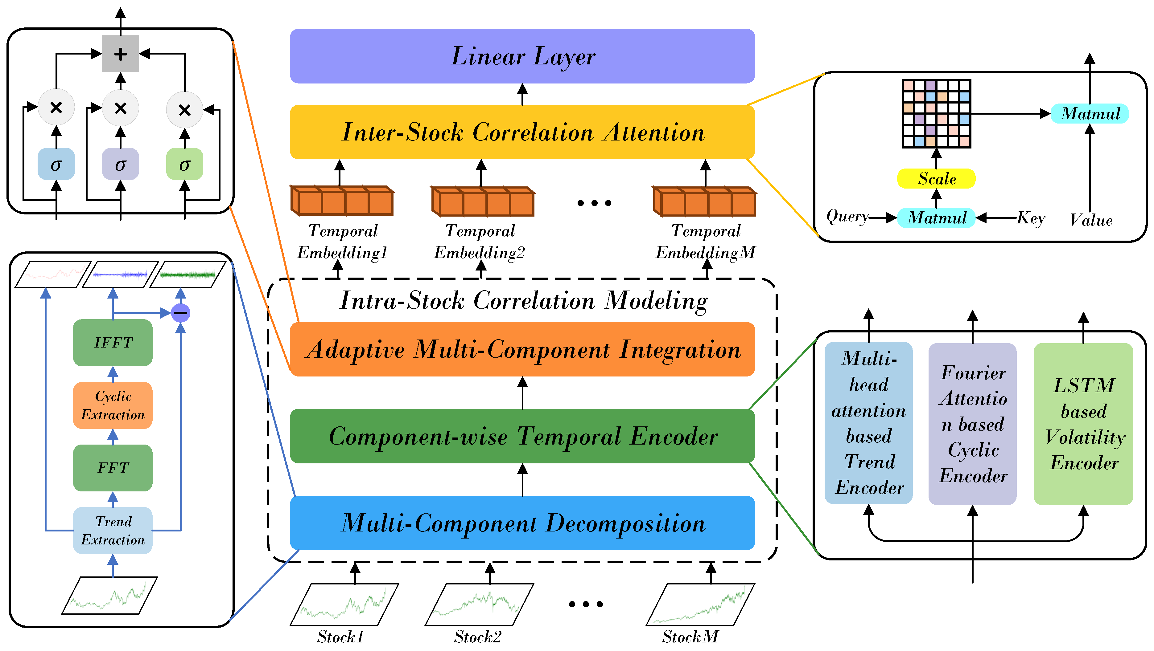
The overall framework of the proposed Hybrid Relational Transformer (HRformer) is illustrated in Figure 1. Considering the intricate and heterogeneous temporal behaviors in stock movements, HRformer first performs component-level decoupling to enhance its ability to model diverse fluctuations. Specifically, a Multi-Component Decomposition Layer is designed to extract the intrinsic periodicities of the input sequence in the frequency domain, while simultaneously separating the trend, cyclic, and volatility components for further representation learning. The decomposed components are then passed into the Component-wise Temporal Encoder (CTE), which independently models their temporal dependencies and internal dynamics. Subsequently, the Adaptive Multi-Component Integration (AMCI) mechanism adaptively fuses the encoded representations, dynamically adjusting each component’s contribution according to its relevance at different time steps. Finally, the Inter-Stock Correlation Attention (ISCA) module captures the relational dependencies among multiple stocks, modeling cross-stock correlations and collective market co-movements in an end-to-end fashion. Overall, HRformer provides a unified framework that jointly models intra-stock temporal structures and inter-stock relationships, enabling a more comprehensive understanding of complex financial time series.

Figure 1. The overall architecture of the HRformer framework.

4.1. Multi-Component Decomposition Layer

The Multi-Component Decomposition Layer is developed to decompose the input stock time series into its essential elements—the trend, cyclic, and volatility components—as shown in Figure 1. This layer integrates several submodules, including a Moving Average Module that extracts long-term trend information, and a Spectral Decomposition Module (SDM) that identifies cyclic patterns and short-term fluctuations in the frequency domain.

Given an input series ${\mathbf{X}}_I\in {\mathbb{R}}^{L\times d}$ of dimension d, a moving average operation is first applied to smooth high-frequency variations and extract the trend component, highlighting its long-term evolution. For a sequence of length L, the process can be expressed as

$${\mathbf{X}}_t=\mathrm{AvgPool}\left(\mathrm{Padding}\left(\mathbf{X}\right)\right)$$

(4)

$${\mathbf{X}}_w=\mathbf{X}-{\mathbf{X}}_t$$

(5)

Here, ${\mathbf{X}}_t$ and ${\mathbf{X}}_w\in {\mathbb{R}}^{L\times d}$ represent the extracted trend and preliminary fluctuation components, respectively. The $\mathrm{AvgPool}(·)$ operation ensures that the smoothed trend preserves the original sequence length through appropriate padding.

Previous studies [24] commonly utilized ${\mathbf{X}}_w$ directly as the seasonal component, which limited the model’s ability to distinguish the diverse fluctuation behaviors in financial data and failed to account for volatility effects. To overcome this limitation, the Multi-Component Decomposition Layer further decomposes ${\mathbf{X}}_w$ using a Fast Fourier Transform (FFT) to isolate periodic and random variations more precisely. The Spectral Decomposition Module (SDM) enhances this process by introducing a locally adaptive thresholding mechanism that adjusts the spectral mask according to the magnitude characteristics in the frequency domain. The procedure is formulated as

$${\mathbf{X}}_f=\mathrm{FFT}\left({\mathbf{X}}_w\right)$$

(6)

$${\mathbf{X}}_{\mathrm{c}},{\mathbf{X}}_{\mathrm{v}}=\mathrm{IFFT}\left(\mathbf{Mask}\left({\mathbf{X}}_f\right)\right)$$

(7)

where, ${\mathbf{X}}_f$ denotes the frequency-domain representation of the preliminary signal, while $\mathrm{Mask}(·)$ selectively preserves dominant periodic frequencies. The inverse FFT reconstructs the cyclic component ${\mathbf{X}}_{\mathrm{c}}$ and the volatility component ${\mathbf{X}}_{\mathrm{v}}$ in the time domain.

To refine the masking process, a dynamic threshold is computed by evaluating the localized spectral energy distribution:

$$T_{\mathrm{l}}=\mathrm{AvgPool}1\mathrm{d}\left(\mathrm{Padding}\right(|{\mathbf{X}}_f\left|\right))$$

(8)

$$T_{\mathrm{d}}={\theta }_{\mathrm{d}}·T_{\mathrm{l}}$$

(9)

$$\mathbf{Mask}=|{\mathbf{X}}_f|>T_{\mathrm{l}}·T_{\mathrm{d}}$$

(10)

In this formulation, $T_{\mathrm{l}}$ represents a local spectral threshold, $T_{\mathrm{d}}$ is a dynamic threshold adjusted based on the data’s frequency distribution, and ${\theta }_{\mathrm{d}}$ is a learnable coefficient optimized during training. The final reconstruction of the cyclic and volatility components is given by

$${\mathbf{X}}_{\mathrm{c}},{\mathbf{X}}_{\mathrm{v}}=\mathrm{IFFT}({\mathbf{X}}_f\odot \mathrm{Mask})$$

(11)

Notably, the frequency masking thresholds in Equations (9)–(11) are manually adjusted based on experimental results during the model validation phase. To ensure effective separation of cyclic and volatility components, we test a range of candidate threshold values on the validation set, with final values determined by balancing two key metrics: the degree of non-overlap between decomposed components (verified via frequency–domain analysis) and the subsequent predictive performance of HRformer (e.g., F1-score on stock trend prediction). The selected thresholds are fixed for the formal training and testing phases to maintain experimental consistency. Similarly, the moving-average windows (for trend extraction) and FFT cutoff frequencies (for cyclic–volatility separation) in MCDL follow the same logic: they are manually tuned during validation, tested on the validation set, and fixed for training/testing after being determined via the same two metrics. FFT and moving-average filters are chosen over EMD/STL/wavelets here: they fit end-to-end optimization (adaptive methods can’t embed for gradient propagation) and avoid leakage (EMD uses future data, while these filters only rely on historical sliding windows). Moreover, the MCDL’s decomposition is fully differentiable and integrated into HRformer’s end-to-end optimization-embedded as a core network part, not a static preprocessing step, and jointly learned with other modules.

This multi-scale decomposition strategy enables the Multi-Component Decomposition Layer to disentangle stock time series into interpretable components, effectively capturing long-term trends, recurrent cycles, and rapid fluctuations. The resulting representation offers a more structured and informative foundation for subsequent temporal modeling and correlation learning. Specifically, the trend component reflects the long-term evolution of stock prices, representing the company’s fundamental growth and overall market perception. The cyclic component captures periodic patterns that often emerge in sectors sensitive to commodity or energy prices—such as mining, coal, and oil—where market movements exhibit clear cyclical behaviors. In contrast, the volatility component characterizes short-term price fluctuations, whose analysis helps mitigate the influence of transient noise on prediction and trading strategies, leading to more stable and realistic forecasting outcomes.

Mathematically, for input time series $X_t$, its frequency–domain representation $X_f$ (via FFT) is partitioned into low-frequency (trend $X_T$), mid-frequency (cyclic $X_C$), and high-frequency (volatility $X_V$) components using threshold masking, satisfying $X_f=X_T+X_C+X_V$ with non-overlapping supports ($\mathrm{supp}\left(X_T\right)\cap \mathrm{supp}\left(X_C\right)\cap \mathrm{supp}\left(X_V\right)=\varnothing$). This finer frequency resolution covers a more comprehensive frequency space than the ‘trend-seasonal’ dichotomy in FEDformer/TDformer, ensuring independent learning of multi-scale dynamics.

When applied to non-stationary price data (the input targeted by our framework), this decomposition operates exclusively on the real-time sliding input window (e.g., 48-day historical price window per sample). As the window updates with new historical data, the module re-computes trend, cyclic, and volatility components to dynamically reflect the latest non-stationary changes (e.g., trend shifts, volatility spikes). The subsequent Adaptive Multi-Component Integration (AMCI) module further adjusts the weight of each decomposed component in real time (e.g., increasing the weight of the volatility component during market turbulence), forming a ’real-time decomposition + dynamic fusion’ mechanism that is well-suited to non-stationary price data.

4.2. Component-Wise Temporal Encoder

After the Multi-Component Decomposition Layer decomposes the stock time series, the data is separated into three distinct representations corresponding to the trend, cyclic, and volatility components: ${\mathbf{X}}_{\mathrm{t}},{\mathbf{X}}_{\mathrm{c}},{\mathbf{X}}_{\mathrm{v}}\in {\mathbb{R}}^{L\times d}$, respectively. Each component characterizes different temporal behaviors of the original sequence and is therefore modeled independently to extract fine-grained temporal dependencies.

The Component-wise Temporal Encoder processes the three components—trend ($\mathbf{X}\mathrm{t}$), cyclic ($\mathbf{X}\mathrm{c}$), and volatility (${\mathbf{X}}_{\mathrm{v}}$)—produced by the decomposition layer. The trend component reflects long-term stable dynamics and exhibits relatively smooth variations over time, representing the underlying growth tendency of the stock. The cyclic component captures recurrent, periodic fluctuations driven by sectoral or macroeconomic cycles, while the volatility component characterizes short-term, often abrupt and irregular price movements. Since these three components differ significantly in their temporal behaviors and statistical properties, it is essential to design specialized encoders for each of them: the trend component is modeled with a Transformer encoder to capture global dependencies, the cyclic component is processed via Fourier-based attention to emphasize periodic patterns, and the volatility component is represented through a hybrid structure combining RevIN, MLP, and LSTM to model rapid local variations.

4.2.1. Trend Component Processing Module

As illustrated in Figure 2, the temporal evolution of the trend component is modeled using a Transformer encoder, which captures long-range dependencies and structural relationships in stock movements. Its multi-head attention mechanism selectively emphasizes key temporal cues and maintains sensitivity to contextual variations over extended horizons. Unlike recurrent or convolutional models constrained by gradient decay or limited receptive fields, attention enables direct interaction between distant time steps, effectively modeling the smooth and slowly varying characteristics of long-term trends. By assigning different heads to distinct temporal patterns, the Transformer integrates multi-scale dependencies and captures persistent structures. This property has been validated in recent time-series studies [22,25,26], where multi-head attention demonstrates strong capability in representing stable, low-frequency trend components in sequential data.

Figure 2. The framework of the Trend Component Processing Module.

Formally, the attention mechanism uses three linear projections—Query ($\mathbf{Q}$), Key ($\mathbf{K}$), and Value ($\mathbf{V}$)—defined as

$$\mathbf{Q}={\mathbf{X}}_{\mathrm{t}}{\mathbf{W}}^Q,\mathbf{K}={\mathbf{X}}_{\mathrm{t}}{\mathbf{W}}^K,\mathbf{V}={\mathbf{X}}_{\mathrm{t}}{\mathbf{W}}^V$$

(12)

where ${\mathbf{W}}^Q$, ${\mathbf{W}}^K$, and ${\mathbf{W}}^V$ are learnable weight matrices for the projections.

The self-attention operation computes relevance-based weightings between temporal positions:

$$\mathrm{Attention}(\mathbf{Q},\mathbf{K},\mathbf{V})=\mathrm{softmax}\left({\displaystyle \frac{\mathbf{Q}{\mathbf{K}}^T}{\sqrt{d_k}}}\right)\mathbf{V}$$

(13)

Given an initial hidden representation ${\mathbf{H}}^0={\mathbf{X}}_{\mathrm{t}}$, each layer l of the encoder performs:

$${\mathbf{H}}^l=\mathrm{LayerNorm}({\mathbf{H}}^{l-1}+\mathrm{Attention}({\mathbf{Q}}^{l-1},{\mathbf{K}}^{l-1},{\mathbf{V}}^{l-1}))$$

(14)

$${\mathbf{H}}^l=\mathrm{LayerNorm}({\mathbf{H}}^l+\mathrm{FeedForward}\left({\mathbf{H}}^l\right))$$

(15)

where $\mathrm{FeedForward}(·)$ denotes the position-wise transformation layer. The final output ${\mathbf{H}}^L$ represents the refined trend representation containing long-term dependencies for downstream forecasting.

4.2.2. Cyclic Component Processing Module

As illustrated in Figure 3, the Cyclic Component Processing Module aims to learn periodic regularities within stock behavior. Starting from the cyclic component ${\mathbf{X}}_{\mathrm{c}}$ obtained through decomposition, Fourier Attention (FA) [24] is employed to enhance modeling of frequency–domain characteristics, enabling effective detection of recurring cycles and harmonic patterns. By operating in the Fourier domain, FA transforms temporal correlations into spectral representations, where periodic information can be expressed more compactly through dominant frequency components. This frequency-domain processing allows the model to capture periodic dependencies without relying solely on local temporal correlations, overcoming the limitations of purely time–domain attention.

Figure 3. The framework of the Cyclic Component Processing Module.

The initial state ${\mathbf{S}}^0={\mathbf{X}}_{\mathrm{c}}$ is iteratively updated across layers:

$${\mathbf{S}}^l=\mathrm{LayerNorm}({\mathbf{S}}^{l-1}+\mathrm{FourierAttention}\left({\mathbf{S}}^{l-1}\right))$$

(16)

$${\mathbf{S}}^l=\mathrm{LayerNorm}({\mathbf{S}}^l+\mathrm{FeedForward}\left({\mathbf{S}}^l\right))$$

(17)

The final hidden state ${\mathbf{S}}^L$ captures dominant cyclic trends while filtering high-frequency noise, ensuring robust representation of multi-scale periodicity. These refined cyclic features complement the trend and volatility representations, improving the model’s ability to capture market rhythm and recurrence patterns.

4.2.3. Volatility Component Processing Module

As illustrated in Figure 4, the Volatility Component Processing Module addresses rapid fluctuations and irregular variations that characterize financial time series. Since short-term volatility often exhibits abrupt local changes and varying data scales, Reversible Instance Normalization (RevIN) is first applied to stabilize the distribution and remove statistical shifts across time, ensuring the data is suitable for further modeling. This step (applied to the volatility component extracted via MCDL) also addresses non-stationarity of raw OHLC data: it eliminates cross-asset scale differences and temporal statistical shifts, while trend/cyclic components are processed by dedicated encoders (Transformer, Fourier Attention) to capture inherent dynamics. The final fused embeddings via AMCI reflect relative patterns (e.g., trend strength, volatility intensity) rather than absolute prices, ensuring cross-asset comparability. The Long Short-Term Memory (LSTM) network is then employed to capture short-term temporal dependencies, as its gated structure effectively models rapid, transient dynamics within limited time windows. Finally, the Multi-Layer Perceptron (MLP) complements this process by learning nonlinear mappings from the normalized and temporally encoded features, providing robustness for handling random and irregular variations inherent in the volatility component.

Figure 4. The framework of the Volatility Component Processing Module.

Starting with ${\mathbf{X}}_{\mathrm{v}}$ from the decomposition layer, normalization is first applied:

$${\mathbf{X}}_{\mathrm{v}}^{\mathrm{norm}}=\mathrm{RevIN}({\mathbf{X}}_{\mathrm{v}},\mathrm{norm})$$

(18)

RevIN reduces statistical shifts and mitigates distributional non-stationarity, facilitating stable feature extraction. The normalized representation is then projected through the MLP:

$${\mathbf{H}}_0={\mathbf{X}}_{\mathrm{v}}^{\mathrm{norm}}$$

(19)

$${\mathbf{H}}_l=\sigma ({\mathbf{W}}_l{\mathbf{H}}_{l-1}+{\mathbf{b}}_l)$$

(20)

where $\sigma (·)$ denotes a nonlinear activation (e.g., ReLU). Subsequently, an LSTM layer captures temporal dependencies within the volatility sequence:

$${\mathbf{H}}_{\mathrm{LSTM}}=\mathrm{LSTM}\left({\mathbf{H}}_L\right)$$

(21)

Finally, a second normalization and MLP stage refine the output:

$${\mathbf{R}}^{\mathrm{l}}=\mathrm{MLP}\left(\mathrm{RevIN}({\mathbf{H}}_{\mathrm{LSTM}},\mathrm{norm})\right)$$

(22)

This module produces expressive volatility representations that preserve essential short-term dynamics while suppressing noise. When integrated with the trend and cyclic representations, the resulting encoded features form a comprehensive and temporally consistent basis for downstream stock forecasting.

4.3. Adaptive Multi-Component Integration

After obtaining the feature representations of the trend, cyclic, and volatility components, the next step is to integrate them into a unified temporal representation of stock dynamics. Since different stocks exhibit distinct behavioral patterns—growth-oriented stocks are typically dominated by long-term trends, resource-based stocks often follow cyclical fluctuations driven by commodity prices, and certain stocks display strong short-term volatility due to market shocks—the relative importance of each component varies across stocks and over time. To address this heterogeneity, the Adaptive Multi-Component Integration (AMCI) module dynamically allocates component weights for each stock and adaptively adjusts them over time, ensuring that the most relevant temporal information is emphasized at every moment. The integrated output is subsequently fed into the Inter-Stock Correlation Attention (ISCA) module to capture inter-stock dependencies and relational structures.

In the HRformer framework, after the Component-wise Temporal Encoder models the temporal dependencies of each component independently, AMCI adaptively merges these representations through a learnable gating mechanism. This mechanism regulates the information flow from each component, thereby balancing their individual contributions to reflect the overall market state more effectively.

For each time step t, a set of gating coefficients is computed to determine the relative importance of the trend, cyclic, and volatility components. These gating signals are generated via trainable linear transformations followed by a sigmoid activation, which bounds their values between 0 and 1, allowing soft and continuous control over component fusion.

Formally, the adaptive fusion process can be expressed as

$$g_t^T=\sigma ({\mathbf{W}}^T·{\mathbf{H}}^l+{\mathbf{b}}^T)$$

(23)

$$g_t^C=\sigma ({\mathbf{W}}^C·{\mathbf{S}}^l+{\mathbf{b}}^C)$$

(24)

$$g_t^V=\sigma ({\mathbf{W}}^V·{\mathbf{R}}^l+{\mathbf{b}}^V)$$

(25)

$${\mathbf{Z}}_t=g_t^T\odot {\mathbf{H}}^l+g_t^C\odot {\mathbf{S}}^l+g_t^V\odot {\mathbf{R}}^l$$

(26)

Here, $\sigma (·)$ denotes the sigmoid activation function, and ⊙ represents element-wise multiplication. The gating variables $g_t^T$, $g_t^C$, and $g_t^V$ correspond to the attention weights of the trend, cyclic, and volatility components, respectively. These parameters are dynamically adjusted according to the temporal and contextual patterns of the stock data.

From an expressiveness perspective, AMCI’s output $Z_t=g_T\left(t\right)\odot H_T+g_C\left(t\right)\odot H_C+g_V\left(t\right)\odot H_V$ (with time-dependent gating $g_T,g_C,g_V$) belongs to a time-varying mixture kernel, enabling adaptive linear subspace learning per time step—outperforming fixed-weight fusion in FEDformer/TDformer. Information-theoretically, frequency-domain non-overlapping of components ensures low redundancy; adaptive gating further minimizes redundant information during fusion, maximizing effective information retention.

Through this mechanism, AMCI enables the model to flexibly recalibrate the contribution of each temporal component at every moment, effectively capturing both stable and transient market behaviors. The resulting fused representation ${\mathbf{Z}}_t$ encapsulates comprehensive temporal dependencies derived from all components, serving as an informative input for the Inter-Stock Correlation Attention (ISCA) to further learn spatial correlations among multiple stocks.

4.4. Inter-Stock Correlation Attention

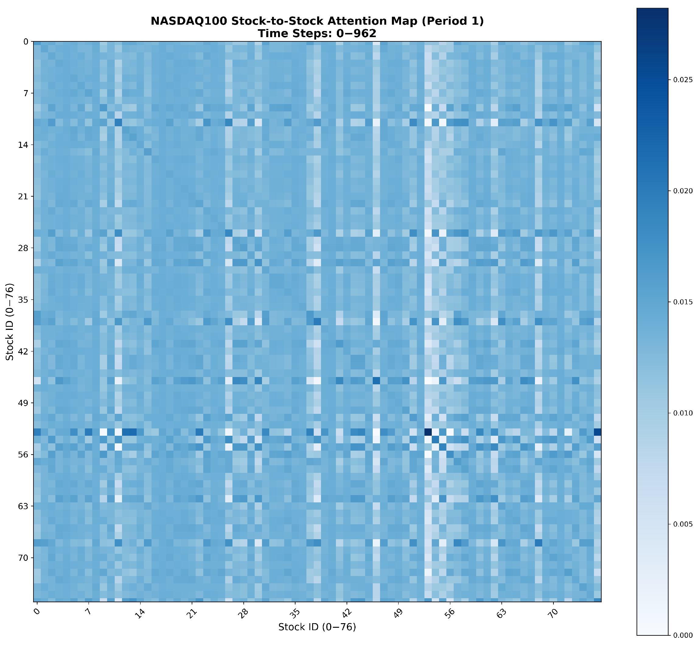
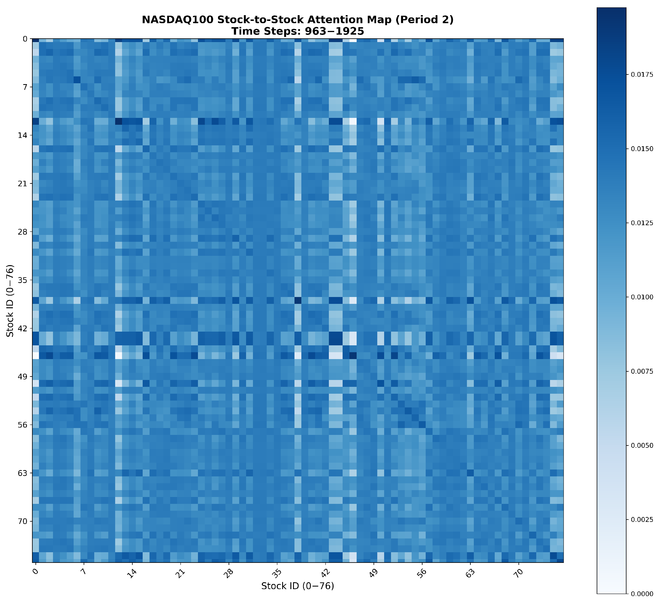
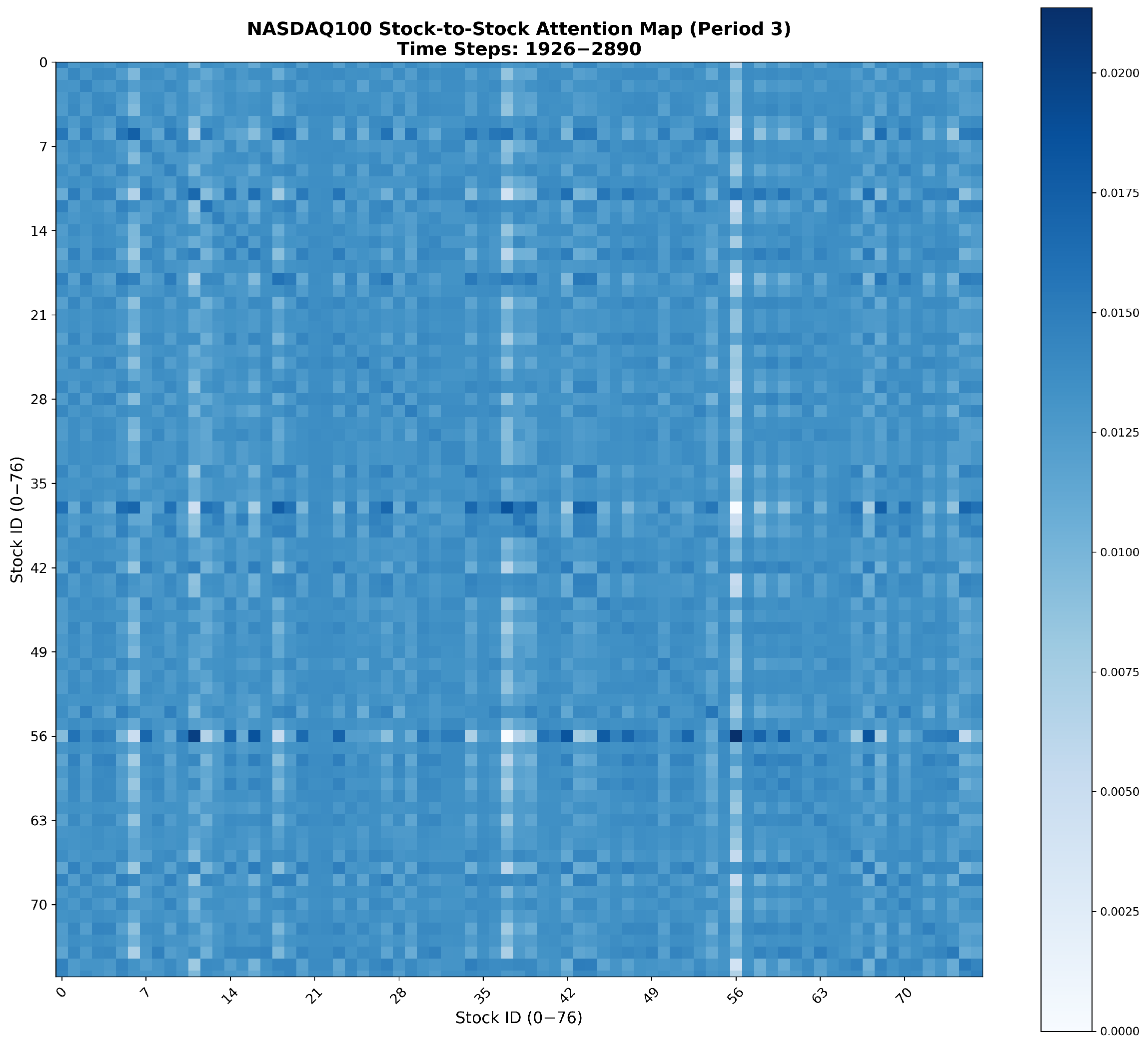
In financial markets, stocks rarely move independently—companies within similar sectors or along the same industrial chain often exhibit strong interdependencies, as upstream and downstream firms are influenced by shared market drivers such as demand fluctuations, raw material prices, or macroeconomic events. These inter-stock correlations form the structural backbone of market dynamics and significantly affect joint price movements across related assets. After the integration of the trend, cyclic, and volatility components through the Adaptive Multi-Component Integration module, the resulting comprehensive temporal features are passed into the Inter-Stock Correlation Attention (ISCA) module. ISCA operates on these normalized temporal embeddings (not raw prices): as shown in Appendix A (attention heatmaps of correlated stocks), it captures meaningful cross-stock dependencies, e.g., NASDAQ100 technology stocks exhibit higher mutual attention weights, aligning with real industry linkages, validating interpretable inter-asset relationships from processed embeddings. This module explicitly learns the spatial dependencies and correlation structures among multiple stocks, enabling the model to capture complex interrelationships and market co-movements that temporal modeling alone cannot fully represent.

To effectively model these cross-stock dependencies, ISCA adopts a mechanism inspired by the iTransformer approach [25]. Specifically, the input dimensions are rearranged from $[B,S,F]$ to $[S,B,F]$, where B is the batch size, S denotes the sequence length, and F represents the feature dimension. This transposition enables the model to treat each stock as a distinct token, allowing the multi-head attention mechanism to learn inter-stock correlations in a structured and data-driven manner.

4.4.1. Multi-Head Attention Mechanism

The foundation of ISCA is the multi-head scaled dot-product attention, which facilitates the modeling of relational dependencies between different stocks. For a given set of combined stock features, the Query (Q), Key (K), and Value (V) matrices are generated such that $Q,K,V\in {\mathbb{R}}^{M\times T\times N}$, where M represents the number of stocks, T is the temporal length, and N is the feature dimension.

The core attention computation is formulated as

$$\mathrm{Attention}(Q,K,V)=\mathrm{softmax}\left({\displaystyle \frac{Q{K}^T}{\sqrt{d_k}}}\right)V$$

(27)

where $d_k$ denotes the dimension of the key vectors. In this setup, Q and K correspond to individual stocks, enabling the attention scores to represent pairwise stock correlations. By multiplying these attention weights with the value matrix V, ISCA constructs enhanced stock representations that embed spatial dependencies and relational dynamics across the market.

This operation captures joint cross-stock correlations $\mathbb{E}\left[X_i{X}_j^{\top }\right|X_t]$, introducing a spatial coupling term to temporal features. Theoretically, HRformer’s representational family ${\mathcal{F}}_{\mathrm{HRformer}}={\mathcal{F}}_{\mathrm{temporal}}\circ {\mathcal{F}}_{\mathrm{spatial}}$ contains FEDformer’s pure temporal family (${\mathcal{F}}_{\mathrm{FEDformer}}\subset {\mathcal{F}}_{\mathrm{HRformer}}$), proving richer expressiveness. Information-theoretically, ISCA maximizes mutual information $I(s_i;s_j|X_t)$ between stock pairs, capturing implicit market correlations (e.g., industry linkages) absent in FEDformer/TDformer.

To enrich the expressiveness of learned dependencies, multiple attention heads operate in parallel. Each head captures correlations from a distinct subspace, and their outputs are concatenated to form the aggregated multi-head attention feature:

$$\mathbf{Z}=\mathrm{MultiHead}(Q,K,V)=\mathrm{Concat}({\mathrm{head}}_1,{\mathrm{head}}_2,\dots ,{\mathrm{head}}_h)W^O$$

(28)

This parallel structure allows the model to simultaneously attend to diverse market interactions, enhancing robustness and predictive accuracy by leveraging multi-perspective relational features.

4.4.2. Feed-Forward Network and Output Projection

Following the attention computation, the aggregated features for each stock are refined through a Feed-Forward Network (FFN) to capture higher-order abstractions. The FFN consists of two fully connected layers with a non-linear activation in between:

$$\mathbf{F}\left(\mathbf{Z}\right)=max(0,\mathbf{Z}{W}_1+b_1)W_2+b_2$$

(29)

where $\mathbf{Z}$ denotes the multi-head attention output, $W_1$ and $W_2$ are learnable weight matrices, and $b_1$, $b_2$ are bias terms. The FFN enhances the representational capacity of each stock token, ensuring the learned embeddings incorporate both temporal–spatial dependencies.

Finally, the processed features are projected through a linear transformation layer (denoted as projector2) to map the hidden representations into the output space for classification. A log_softmax function is applied to convert the logits into probability distributions that indicate the likelihood of upward or downward price movement:

$$\mathrm{softmax}\left(x_i\right)={\displaystyle \frac{exp\left(x_i\right)}{{\sum }_{j=1}^{n}exp\left(x_j\right)}}$$

(30)

Through this design, the Inter-Stock Correlation Attention module effectively integrates both temporal–spatial information, enabling the HRformer to model intricate market co-movements and achieve robust, data-driven stock trend prediction.

5. Experiments

5.1. Datasets

To validate the effectiveness of the proposed Hybrid Relational Transformer (HRformer), we conduct experiments on two major markets: CSI300 (China) and NASDAQ100 (United States). CSI300 reflects the performance of leading A-share stocks from the Shanghai and Shenzhen Stock Exchanges. CSI300 data are obtained from Baostock (http://www.baostock.com, accessed on 23 January 2025), and NASDAQ100 data are obtained from Yahoo Finance (https://finance.yahoo.com, accessed on 26 January 2025). The HRformer’s source code is publicly available at: https://github.com/2276660829/RTDformer.git (accessed on 10 October 2025).

The datasets span 2010–2024, covering 155 CSI300 stocks and 77 NASDAQ100 stocks. To avoid data leakage, we split each dataset chronologically into training, validation, and test subsets with ratios of 70%, 20%, and 10%. Daily features include open, close, high, and low prices. Stocks with incomplete histories or delistings during the evaluation window (4 January 2010–5 June 2024) are excluded. Table 1 reports summary statistics. We use Label_0 and Label_1 to denote ground-truth movement over a future horizon T: Label_0 indicates a decrease or no change, and Label_1 indicates an increase.

Table 1. Details of the dataset.

Dataset		Time Interval	Length	num_stocks	Label_0	Label_1
CSI300	Train set	4 January 2010–29 August 2017	1719	230	148,955	139,500
	Valid set	30 August 2017–15 June 2021	873	230	70,267	72,023
	Test set	16 June 2021–5 June 2024	673	230	54,006	57,749
NASDAQ100	Train set	2 August 2010–1 August 2019	2124	77	70,257	104,225
	Valid set	2 August 2019–10 July 2022	692	77	26,694	30,209
	Test set	11 July 2022–5 June 2024	433	77	18,569	18,391

5.2. Evaluation Metrics

We evaluate classification performance using Accuracy (ACC), Precision (PRE), Recall (REC), and F1-score (F1):

• Accuracy:

  $$\mathrm{ACC}={\displaystyle \frac{\mathrm{TP}+\mathrm{TN}}{\mathrm{TP}+\mathrm{FP}+\mathrm{TN}+\mathrm{FN}}},$$

  (31)

  where TP, TN, FP, and FN denote true positives, true negatives, false positives, and false negatives.
• Precision:

  $$\mathrm{PRE}={\displaystyle \frac{\mathrm{TP}}{\mathrm{TP}+\mathrm{FP}}}.$$

  (32)
• Recall:

  $$\mathrm{REC}={\displaystyle \frac{\mathrm{TP}}{\mathrm{TP}+\mathrm{FN}}}.$$

  (33)
• F1-score:

  $$\mathrm{F}1={\displaystyle \frac{2·\mathrm{PRE}·\mathrm{REC}}{\mathrm{PRE}+\mathrm{REC}}}.$$

  (34)

For backtesting, we adopt a 48-day buy–hold–sell strategy over the test period and report the following:

• Average Maximum Drawdown (AMDD): average of maximum peak-to-trough declines,

  $$\mathrm{AMDD}=\underset{t\in [0,T]}{max}\left({\displaystyle \frac{P_{max,t}-P_{min,t}}{P_{max,t}}}\right),$$

  (35)

  where $P_{max,t}$ is the peak prior to a drawdown and $P_{min,t}$ is the subsequent trough.
• Sharpe Ratio (SR): annualized risk-adjusted return,

  $$\mathrm{SR}={\displaystyle \frac{R_p-R_f}{{\sigma }_p}}\times \sqrt{252},$$

  (36)

  where $R_p$ is portfolio return, $R_f$ is the risk-free rate, and ${\sigma }_p$ is the standard deviation of excess returns.
• Annualized Return (AR): annualized profitability assuming 252 trading days,

  $$\mathrm{AR}={\left({\displaystyle \frac{P_{\mathrm{end}}}{P_{\mathrm{start}}}}\right)}^{{\displaystyle \frac{252}{T}}}-1,$$

  (37)

  where $P_{\mathrm{start}}$ and $P_{\mathrm{end}}$ are initial and final portfolio values, and T is the holding length (days).
• Final Accumulated Portfolio Value (fAPV):

  $$\mathrm{fAPV}={\displaystyle \frac{P_{\mathrm{end}}}{P_{\mathrm{start}}}}.$$

  (38)

Higher SR indicates better risk-adjusted returns; lower AMDD reflects improved capital preservation; higher AR and fAPV indicate stronger overall profitability.

5.3. Compared Methods

We compare HRformer with representative baselines. All implementations follow recommended settings from the original papers and are further tuned on validation sets.

• Transformer: standard self-attention model for global dependency modeling.
• FEDformer: frequency-enhanced decomposition with Transformer to capture global and local dependencies.
• StockMixer: integrates temporal and cross-sectional mixing to model stock-specific and market-wide signals.
• TDformer: temporal decomposition within a Transformer backbone for multi-scale dependency modeling.
• FourierGNN: combines Fourier analysis and graph neural networks to model periodic patterns and cross-stock relations.
• iTransformer: applies attention to transposed dimensions for multivariate dependency modeling.
• DLinear: linear heads over decomposed components for efficient long-horizon forecasting.
• edRVFL: extreme deep random vector functional link network with randomized layers and direct connections.
• TCN: dilated causal convolutions with residual blocks for parallel long-range sequence modeling.

5.4. Implementation Details

HRformer and baselines are implemented in Python 3.10.14; deep learning models use PyTorch 2.1.2 with an NVIDIA GeForce RTX 4090 (24 GB). HRformer is trained with Adam (initial learning rate $1\times {10}^{-3}$). The look-back window for historical context is 96 days; the input window is 48 days; the prediction horizon is 48 days (aligned with the trading cycle). The number of attention heads is 8. These settings balance model capacity and efficiency. A comprehensive hyperparameter summary is provided in Table 2.

Table 2. Model Configuration Parameters.

Model	SeqLen	Epoch	Head	Learning Rate	Hidden Size
Transformer [22]	48	30	8	0.0002	512
FEDformer [17]	48	30	8	0.0002	512
TDformer [36]	48	30	8	0.0002	512
FourierGNN [42]	48	30	0	0.0002	64
iTransformer [25]	48	30	8	0.0002	512
StockMixer [24]	48	30	0	0.0002	512
DLinear [31]	48	30	0	0.0002	64
TCN [20]	48	30	0	0.0002	64
edRVFL [21]	48	30	0	0.0002	64
HRformer	48	30	8	0.0002	512

5.5. Backtesting Settings

We simulate a 48-day buy–hold–sell cycle under market-specific trading costs, with a 0.1% trading cost applied to both the CSI300 and NASDAQ100 datasets, for Chinese and U.S. markets. Notably, we tested alternative cycle lengths (12, 24, 48, and 96 days) for this buy–hold–sell strategy prior to finalizing the design, and the 48-day cycle was selected as it achieved the best performance in terms of predictive accuracy and consistency with real-world trading rhythms. On day t, we select top-performing stocks by the predicted 48-day rise probability relative to day $t+1$. For CSI300, we buy the top 10 stocks; for NASDAQ100, we buy the top 20 stocks. Positions are equally weighted—implementing an equal-weight allocation strategy—held for 48 days, then closed; the remaining capital, along with proceeds from the closed positions, is rolled into the next cycleto purchase a new batch of top-ranked stocks based on the latest predicted rise probability, ensuring the trading cycle is fully aligned with the 48-day prediction horizon. This design reflects differing market frictions and allows a fair comparison of profitability and robustness across methods.

• Trading period: July 2022 to June 2024 for both CSI300 and NASDAQ100.
• Stock selection: top 10 (CSI300) or top 20 (NASDAQ100) by predicted rise probability at day t over the next 48 days.

6. Results and Analysis

6.1. Overall Performance

Based on Table 3, HRformer consistently outperforms other models on both datasets across ACC, PRE, REC, and F1. On NASDAQ100, it achieves the highest scores on all four metrics, indicating strong predictive capability in relatively less volatile conditions. On CSI300, which is more volatile, HRformer still ranks first on every metric, demonstrating robustness under challenging market dynamics.

Table 3. Comparisons of predictive performance on NASDAQ100 and CSI300 datasets ($\times {10}^{-2}$).

Model	NASDAQ100				CSI300
	ACC (↑)	PRE (↑)	REC (↑)	F1 (↑)	ACC (↑)	PRE (↑)	REC (↑)	F1 (↑)
Transformer [29]	53.51	61.54	61.11	61.33	51.44	52.76	51.97	52.36
FEDformer [23]	52.96	61.51	58.83	60.14	50.24	51.73	48.47	50.05
TDformer [24]	50.87	61.68	47.94	54.06	51.80	52.26	60.74	56.18
FourierGNN [46]	50.90	60.57	53.37	56.74	51.99	52.71	58.22	55.33
iTransformer [25]	46.86	57.45	45.65	50.88	49.87	51.22	57.67	54.25
StockMixer [47]	46.77	57.79	42.88	49.23	52.49	53.07	56.23	54.88
DLinear [38]	51.40	60.54	61.07	58.19	50.43	51.54	60.65	55.72
TCN [48]	51.98	59.98	61.84	58.75	52.10	52.98	61.00	50.71
edRVFL [49]	51.46	59.88	59.76	56.77	51.96	52.96	58.91	55.78
HRformer	54.91	61.76	66.15	63.88	52.61	53.36	61.95	57.33

Note: ↑ indicates the larger the indicator value, the better; Underline denotes the second-best results; italic denotes the results of HRformer.

StockMixer shows weaker performance on NASDAQ100 but performs relatively better on CSI300, suggesting partial capture of temporal dependencies. Transformer and FEDformer emphasize long-range dependencies and overall trends; while effective in stable markets, they may under-represent short-term, non-stationary fluctuations typical of CSI300, leading to inferior results versus HRformer. Transformer surpasses iTransformer on NASDAQ100 by leveraging long-horizon trends, whereas iTransformer’s interactive attention is less effective amid CSI300’s volatility where fine-grained fluctuations dominate. FourierGNN, which blends Fourier analysis with GNNs, struggles with chaotic, non-periodic behaviors prevalent in CSI300. DLinear is balanced but limited by linear modeling of complex short-term patterns. TCN captures local patterns yet its volatility sensitivity causes inconsistent F1 on CSI300. edRVFL remains moderately stable but randomization can dilute feature specificity in turbulent regimes.

Relative to TDformer on NASDAQ100, HRformer improves Accuracy by about 0.83%, Precision by 1.43%, Recall by 2.93%, and F1 by 1.78%; similar gains hold against the next-best Transformer, highlighting HRformer’s superior capacity for stock trend modeling.

6.2. Visualization and Analysis of Stock Price Component Decomposition, Dynamic Weight Distribution, and Periodic Patterns

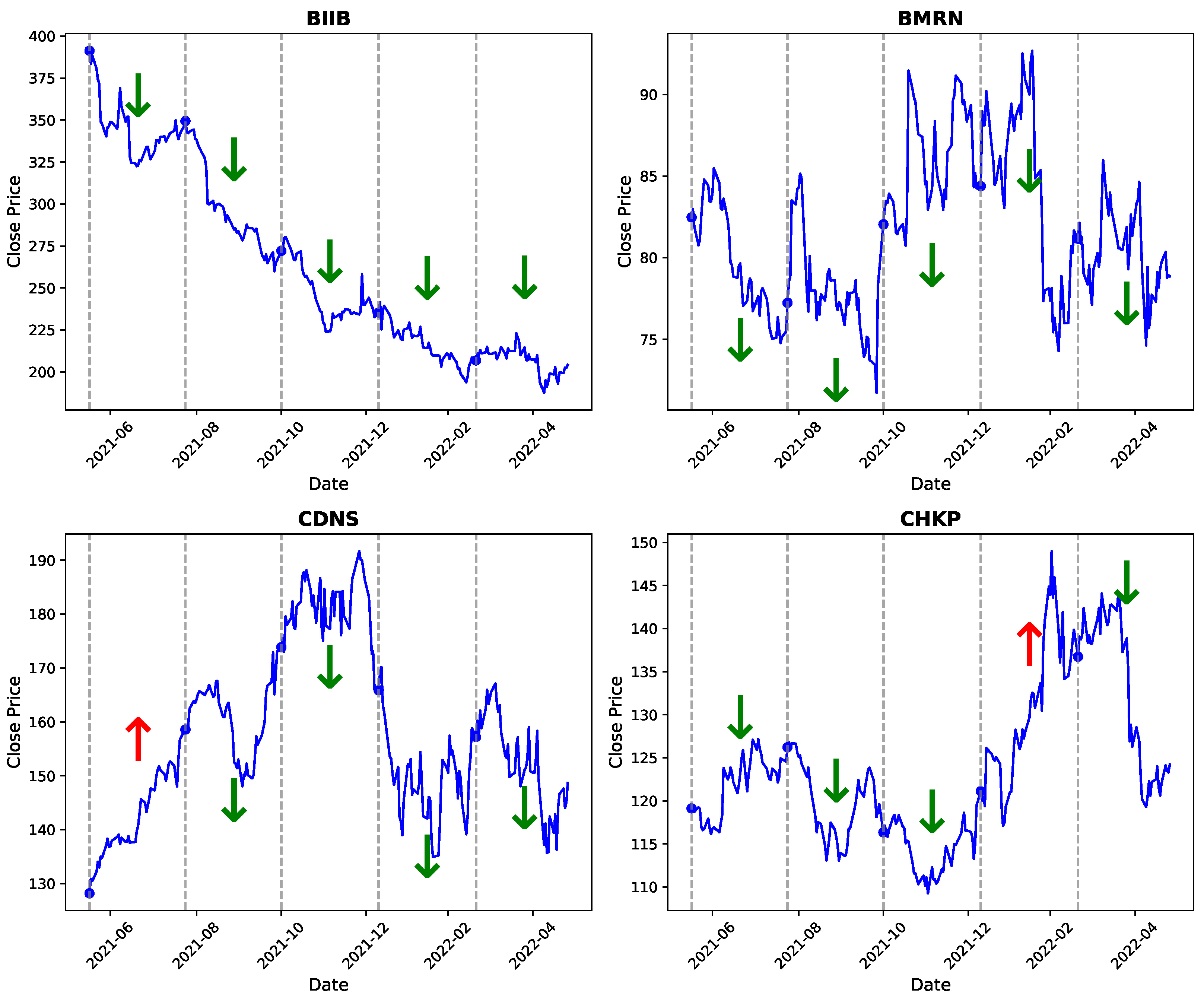
We further demonstrate HRformer’s predictive effectiveness through detailed visualizations. Four representative stocks—BIIB, BMRN, CDNS, and CHKP—were selected to compare actual and predicted price movements over specific time windows.

• Red upward arrows (↑): periods where HRformer predicted a price increase.
• Green downward arrows (↓): periods where HRformer predicted a price decrease.

As shown in Figure 5, HRformer captures both short-term fluctuations and long-term directional trends, validating the combined effectiveness of its decomposition (via the Multi-Component Decomposition Layer) and adaptive fusion (AMCI) mechanisms, along with accurate temporal–spatial modeling.

Figure 5. Visualized trend prediction: arrows indicate model forecasts of upward or downward movement.

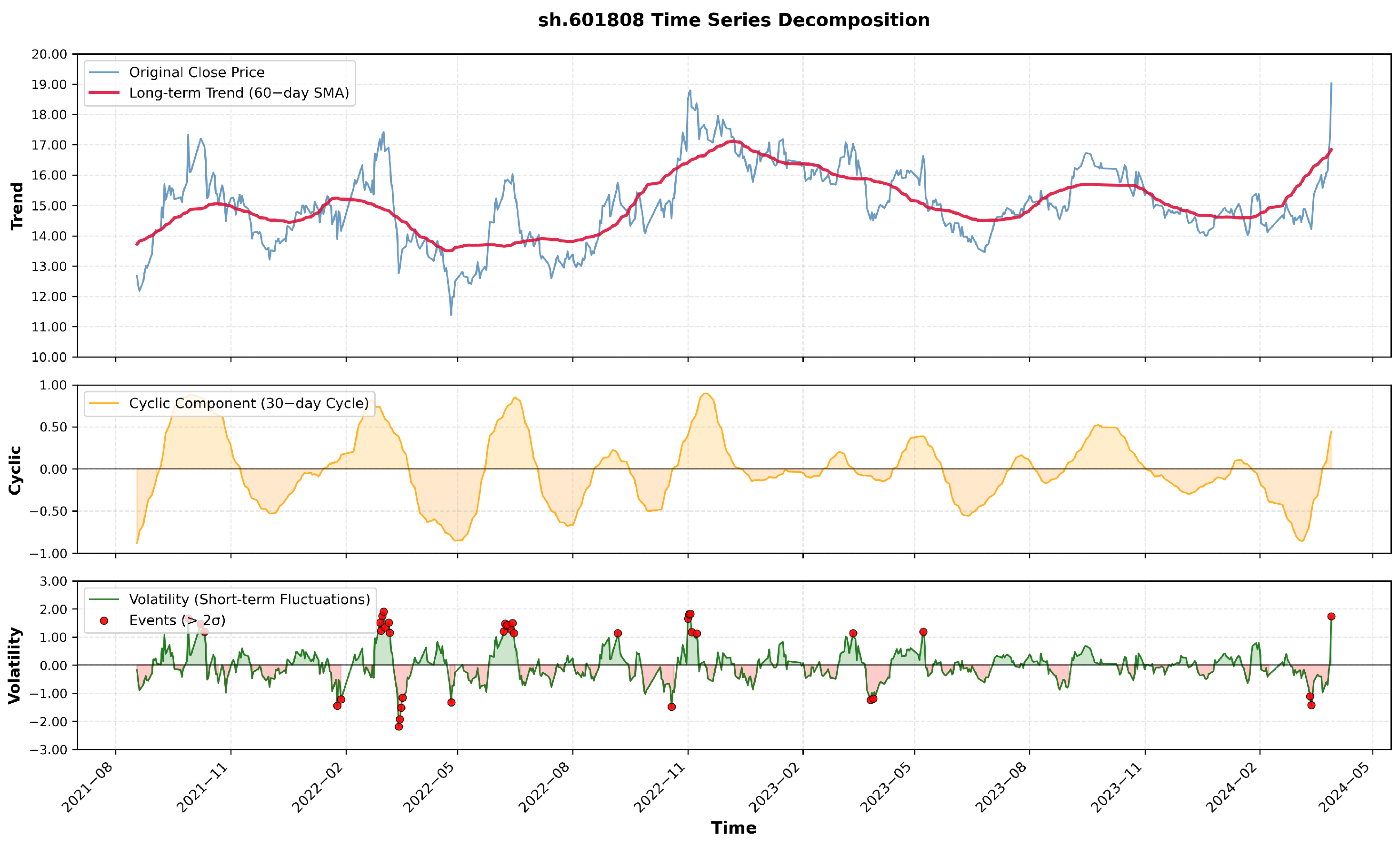
Figure 6 presents the time series decomposition experiment of stock sh.601808 from the CSI300 index, aiming to visualize the Volatility component. It can be observed that the Volatility component is designed to capture short-term fluctuations and reflect unexpected events.

Figure 6. Time series decomposition of stock sh.601808 (CSI300)—visualization of the Volatility component.

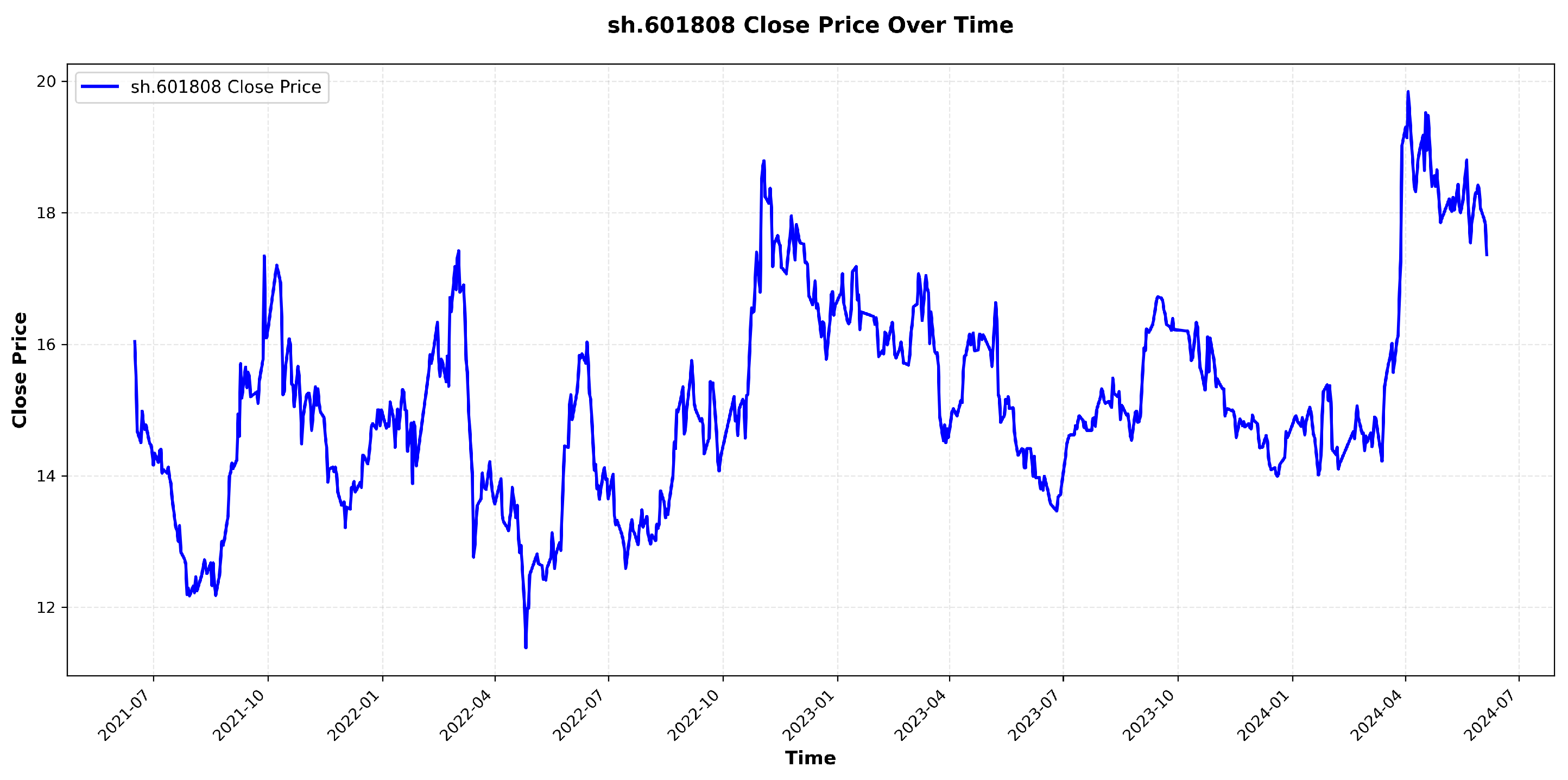
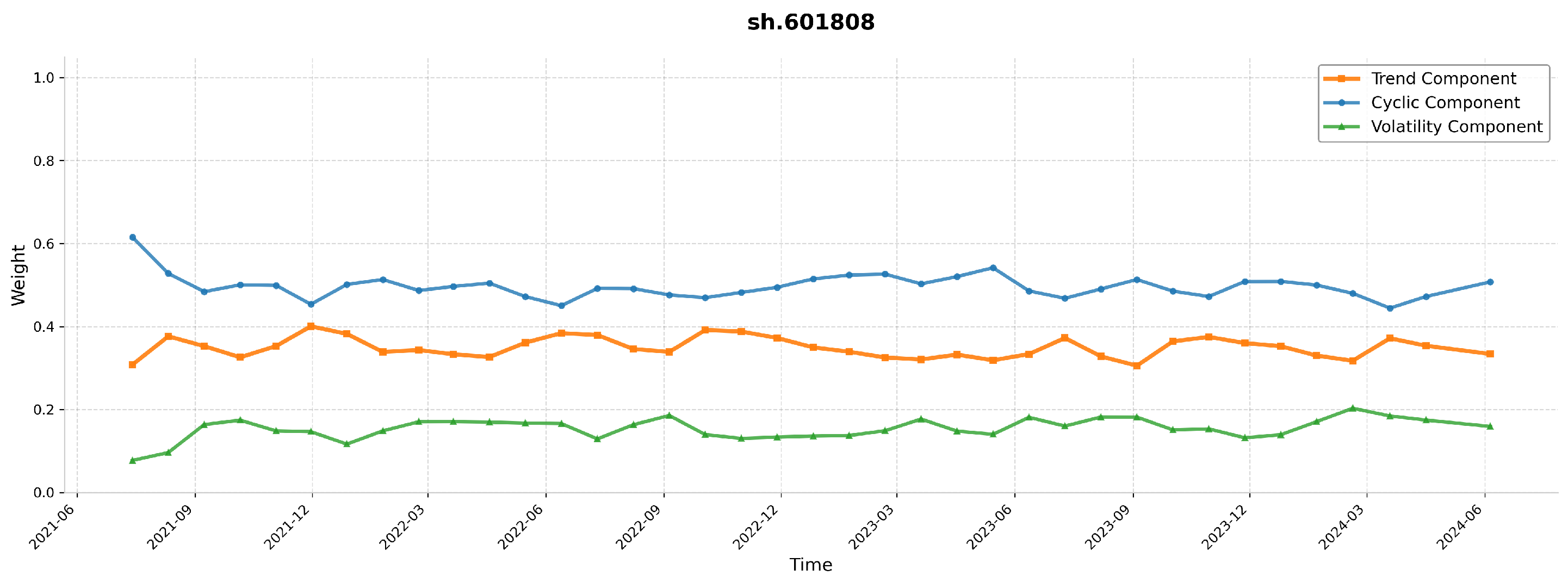
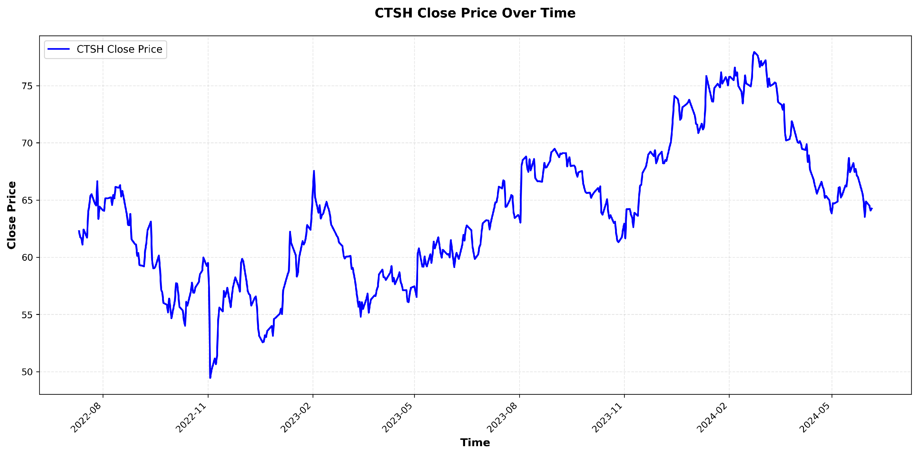
Stock data often exhibit periodic behaviors, though not uniformly across all equities. To verify this, we analyzed the dynamic changes of Trend, Cyclic, and Volatility weight distributions of representative stocks—CTSH from the NASDAQ100 and sh.601808 from the CSI300—under different time periods and volatility regimes. As illustrated in Figure 7, Figure 8, Figure 9 and Figure 10, CTSH shows periodicity in the early stage, shifts to trend-dominant characteristics in the mid-term, and returns to periodicity in the final stage. In contrast, sh.601808 maintains stable periodicity throughout the entire observation period.

Figure 7. Original price of stock sh.601808 (CSI300).

Figure 8. Trend/Cyclic/Volatility weight distribution of sh.601808 (CSI300).

Figure 9. Original price of stock CTSH (NASDAQ100).

Figure 10. Trend/Cyclic/Volatility weight distribution of CTSH (NASDAQ100).

6.3. Backtesting Performance

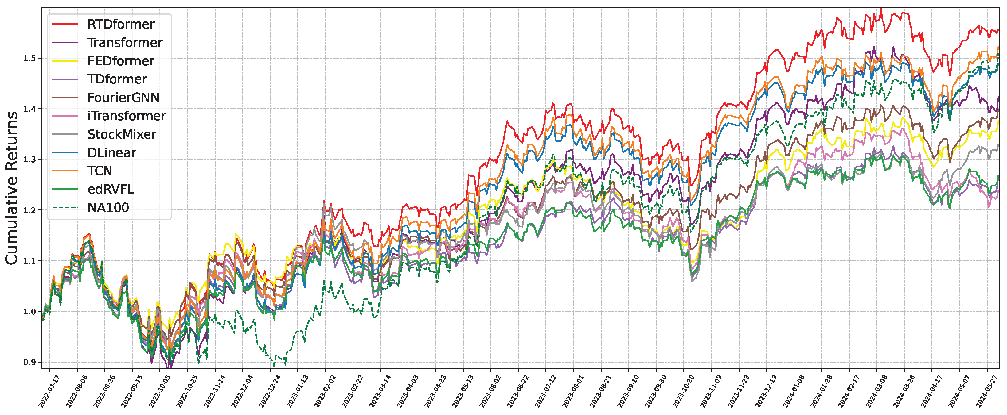
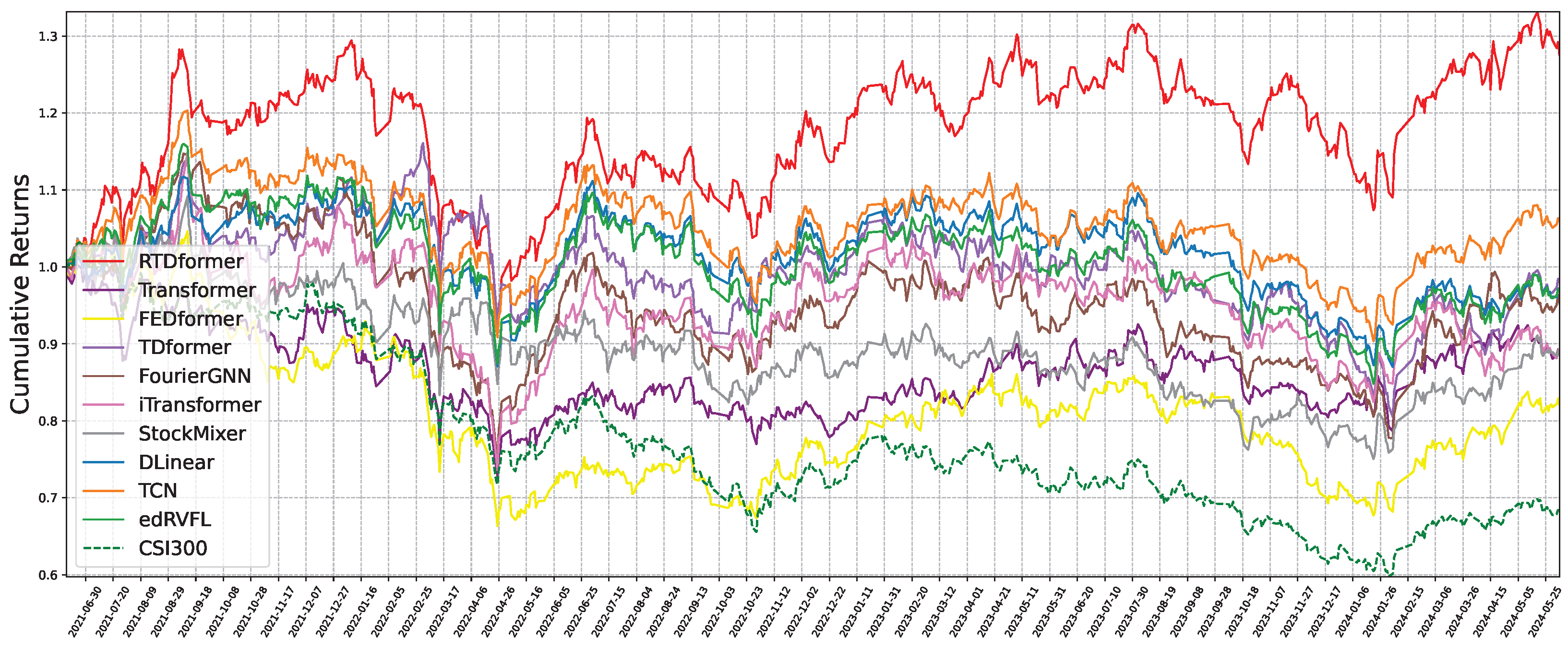
Figure 11 and Figure 12 plot cumulative returns using an identical trading protocol for all methods. HRformer substantially outperforms alternatives in both markets, indicating more profitable stock selection. Table 4 compares profitability metrics (AR, AMDD, SR, fAPV). HRformer achieves the best SR, AR, and fAPV on both datasets and second-best AMDD, reflecting a mild trade-off in drawdown for superior overall returns.

Figure 11. Cumulative return curve from backtesting on NASDAQ100.

Figure 12. Cumulative return curve from backtesting on CSI300.

Table 4. Backtesting performance comparison on NASDAQ100 and CSI300 ($\times {10}^{-2}$).

Model	NASDAQ100				CSI300
	AMDD (↓)	SR (↑)	AR (↑)	fAPV (↑)	AMDD (↓)	SR (↑)	AR (↑)	fAPV (↑)
Transformer [29]	16.53	142.50	20.47	142.58	24.03	−50.77	−4.01	88.96
FEDformer [23]	15.56	119.15	20.30	142.19	35.86	−55.17	−6.70	82.03
TDformer [24]	15.67	113.00	12.69	125.55	24.22	−23.17	−0.69	98.03
FourierGNN [46]	15.24	135.73	20.00	141.51	30.61	−16.83	−1.69	95.25
iTransformer [25]	15.59	111.12	12.00	124.10	29.48	−13.67	−3.92	89.20
StockMixer [47]	17.40	94.70	16.05	132.78	26.57	−64.91	−4.14	88.63
DLinear [38]	15.83	149.04	23.22	148.85	23.40	−7.10	−1.12	96.91
TCN [48]	16.00	151.47	24.55	151.93	24.59	3.62	1.68	105.98
edRVFL [49]	15.60	117.81	12.95	126.27	25.64	−9.30	−1.30	96.89
HRformer	15.53	153.54	26.18	155.72	22.32	53.98	8.88	127.53

Note: ↑ indicates the larger the indicator value, the better; ↓ indicates the smaller the indicator value, the better. Underline denotes the second-best results; bold denotes the results of HRformer.

6.4. Statistical Analysis

A Wilcoxon signed-rank test was performed on paired metric differences across ten runs. As shown in Table 5, HRformer achieved statistically significant improvements (p < 0.05) in both classification (ACC, PRE, F1) and backtesting (ASR, AR, fAPV) metrics compared to all baselines, confirming its consistent superiority.

Table 5. Results of Wilcoxon signed-rank test for NASDAQ100.

Model Comparison	ACC (↑)	PRE (↑)	F1 (↑)	ASR (↑)	AR (↑)	fAPV (↑)
HRformer vs. Transformer	0.002	0.002	0.002	0.002	0.002	0.002
HRformer vs. FEDformer	0.002	0.193	0.002	0.008	0.023	0.023
HRformer vs. TDformer	0.002	0.002	0.002	0.008	0.023	0.023
HRformer vs. FourierGNN	0.004	0.004	0.002	0.002	0.002	0.002
HRformer vs. iTransformer	0.002	0.002	0.002	0.002	0.002	0.002
HRformer vs. StockMixer	0.014	0.020	0.002	0.002	0.002	0.002
HRformer vs. DLinear	0.002	0.002	0.002	0.002	0.004	0.004
HRformer vs. TCN	0.002	0.002	0.002	0.004	0.002	0.002
HRformer vs. edRVFL	0.002	0.002	0.002	0.006	0.004	0.004

Note: ↑ indicates the larger the indicator value, the better.

6.5. Ablation Study

We assess the contribution of each component via ablations:

• HRformer-FFT: remove FFT/IFFT within the Multi-Component Decomposition Layer to test the role of frequency–domain separation of cyclic and volatility components.
• HRformer-VC: remove the volatility component branch to evaluate the impact of short-term fluctuation modeling.
• HRformer-ISCA: remove the Inter-Stock Correlation Attention to test cross-stock spatial dependency modeling.
• HRformer-TA: replace attention in the Component-wise Temporal Encoder with an MLP to test temporal attention effectiveness.

The ablation experiments confirm the necessity of each component in HRformer. The backtesting results of these ablation experiments are presented in Figure 13 and Figure 14, while the performance metrics of the ablation experiments are detailed in Table 6 and Table 7. Consistent with our theoretical claims: removing FFT decomposition (HRformer-FFT) or volatility branch (HRformer-VC) reduces F1-score/Sharpe ratio ($p<0.05$) (validating frequency-domain coverage), while removing ISCA (HRformer-ISCA) weakens cross-stock modeling (validating spatial coupling value)—aligning with mathematical and information-theoretic justifications, and replacing temporal attention with MLP (HRformer-TA) degrades long-range and periodic dependency capture.

Figure 13. Backtesting results of the ablation study on NASDAQ100.

Figure 14. Backtesting results of the ablation study on CSI300.

Table 6. Performance of ablation experiments on NASDAQ100 ($\times {10}^{-2}$).

Model	Acc (↑)	Pre (↑)	Recall (↑)	F1 (↑)	AMDD (↓)	SR (↑)	AR (↑)	fAPV (↑)
HRformer-FFT	53.68	61.67	57.41	59.92	14.55	114.30	14.92	130.32
HRformer-VC	54.82	61.52	59.00	61.18	15.61	152.82	25.65	154.49
HRformer-ISCA	51.90	61.36	54.88	57.94	15.71	91.76	11.24	122.49
HRformer-TA	50.16	60.31	58.44	60.11	15.94	142.37	24.15	150.99
HRformer	54.91	61.76	66.15	63.88	15.53	153.54	26.18	155.72

Note: ↑ indicates the larger the indicator value, the better; ↓ indicates the smaller the indicator value, the better. Underline denotes the second-best results, bold denotes the results of HRformer.

Table 7. Performance of ablation experiments on CSI300 ($\times {10}^{-2}$).

Model	Acc (↑)	Pre (↑)	Recall (↑)	F1 (↑)	AMDD (↓)	SR (↑)	AR (↑)	fAPV (↑)
HRformer-FFT	51.83	51.42	61.07	54.63	21.05	44.01	3.45	110.18
HRformer-VC	52.31	53.17	61.03	56.83	23.43	40.42	7.21	122.00
HRformer-ISCA	51.38	51.84	56.38	55.52	29.44	−41.34	−5.07	86.16
HRformer-TA	51.10	52.34	56.10	54.72	22.70	−21.38	−2.76	92.28
HRformer	52.61	53.36	61.95	57.33	22.32	53.98	8.88	127.53

Note: ↑ indicates the larger the indicator value, the better; ↓ indicates the smaller the indicator value, the better. Underline denotes the second-best results; bold denotes the results of HRformer.

6.6. Parameter Analysis

We analyze the sensitivity of HRformer to the number of attention heads on NASDAQ100 while holding other hyperparameters fixed. As shown in Figure 15, the number of heads substantially influences ACC, PRE, REC, and F1; more heads do not monotonically improve results. We set the number of heads to 8 based on this trade-off.

Figure 15. Impact of the number of attention heads on ACC, PRE, REC, and F1.

6.7. Complexity Analysis

We report model complexity using training time per epoch (time complexity) and parameter count (space complexity). As shown in Table 8, HRformer incurs a moderate increase in computation due to the introduction of the volatility modeling branch after decomposition. However, the added cost remains acceptable relative to its substantial performance improvements. The framework’s robustness and predictive precision outweigh this increase, suggesting that future work can focus on lightweight optimizations for improved efficiency.

Table 8. Complexity analysis of models.

Model	Parameters	One-Epoch Training Time (s)
Transformer [22]	10,532,872	32
FEDformer [17]	10,527,244	33
TDformer [36]	10,865,222	33
FourierGNN [42]	1,897,338	30
iTransformer [24]	6,380,090	27
StockMixer [24]	31,927	33
DLinear [31]	74,506	25
TCN [20]	40,410	23
edRVFL [21]	43,300	23
HRformer	22,462,014	42

6.8. Performance Analysis

As shown in Table 9, HRformer has strong deployment feasibility: its 0.000064 s per-sample latency meets high-frequency trading real-time needs, 3.26 GB max GPU memory supports single-GPU multi-request parallelism, and 22.43 M parameters keep deployment costs low. Its slightly higher overhead than iTransformer and FEDformer stems from the newly added multi-component decomposition (Trend/Cyclic/Volatility separation) and cross-stock correlation attention module—these modules not only increase parameters moderately but also are the key to its superior performance over the two models, with limited overhead growth that does not hinder practical deployment.

Table 9. Computational Cost Analysis of Different Models.

Model	Trainable Parameters	Training Time	Max GPU Memory	Batch Inference Latency	Per-Sample Latency	Throughput (Samples/s)
HRformer	22.43 M	0.05 h	3.26 GB	0.0164 s	0.000064 s	15,640.82
FEDformer	10.53 M	0.03 h	1.98 GB	0.0039 s	0.000015 s	65,701.67
iTransformer	6.35 M	0.02 h	0.19 GB	0.0020 s	0.000008 s	125,617.33

7. Conclusions

This paper introduced the Hybrid Relational Transformer (HRformer) for stock trend prediction, a practical yet challenging task in quantitative investment. Unlike prior approaches that emphasize either short-range variations or long-horizon dependencies, HRformer integrates both by first decomposing time series into trend, cyclic, and volatility components through a Multi-Component Decomposition Layer. This comprehensive separation enables the model to capture complex, dynamic temporal patterns. Each component is then modeled by the Component-wise Temporal Encoder (CTE), and their representations are adaptively fused via the Adaptive Multi-Component Integration (AMCI) mechanism. Finally, Inter-Stock Correlation Attention (ISCA) learns cross-stock spatial dependencies, yielding end-to-end forecasts that reflect both temporal dynamics and inter-asset relationships.

Extensive experiments on CSI300 and NASDAQ100 demonstrate that HRformer consistently outperforms state-of-the-art baselines in classification metrics and backtesting indicators, showing strong robustness under volatile market conditions. The backtesting results further confirm the practical utility of the proposed framework for real-world trading, highlighting its potential to support informed decision-making and improve long-term profitability.

Future work includes considering more diverse trading strategies (e.g., dynamic weight allocation, multi-cycle rebalancing) to explore their impacts on risk-adjusted metrics (Sharpe ratio, maximum drawdown, annualized return)—further aligning HRformer’s evaluation with practical financial settings—and exploring log-return inputs by reconfiguring the Multi-Component Decomposition Layer and retuning encoders for return-series dynamics. Beyond finance, the core HRformer design—multi-component decomposition, component-wise temporal encoding, adaptive fusion, and cross-entity attention—may generalize to other non-stationary domains such as traffic forecasting and battery health estimation.

References

- Song, L.; Li, H.; Chen, S.; Gan, X.; Shi, B.; Ma, J.; Pan, Y.; Wang, X.; Shang, X. Multi-Scale Temporal Neural Network for Stock Trend Prediction Enhanced by Temporal Hyepredge Learning. In Proceedings of the IJCAI, Montreal, QC, Canada, 16–22 August 2025; pp. 3272–3280. [Google Scholar]
- Luo, Y.; Zheng, J.; Yang, Z.; Chen, N.; Wu, D.O. Pleno-Alignment Framework for Stock Trend Prediction. IEEE Trans. Neural Netw. Learn. Syst. 2025, 36, 16604–16618. [Google Scholar] [CrossRef] [PubMed]
- Yi, S.; Chi, J.; Shi, Y.; Zhang, C. Robust stock trend prediction via volatility detection and hierarchical multi-relational hypergraph attention. Knowl. Based Syst. 2025, 329, 114283. [Google Scholar] [CrossRef]
- Liao, S.; Xie, L.; Du, Y.; Chen, S.; Wan, H.; Xu, H. Stock trend prediction based on dynamic hypergraph spatio-temporal network. Appl. Soft Comput. 2024, 154, 111329. [Google Scholar] [CrossRef]
- Du, Y.; Xie, L.; Liao, S.; Chen, S.; Wu, Y.; Xu, H. DTSMLA: A dynamic task scheduling multi-level attention model for stock ranking. Expert Syst. Appl. 2024, 243, 122956. [Google Scholar] [CrossRef]
- Han, H.; Xie, L.; Chen, S.; Xu, H. Stock trend prediction based on industry relationships driven hypergraph attention networks. Appl. Intell. 2023, 53, 29448–29464. [Google Scholar] [CrossRef]
- Almasarweh, M.; Alwadi, S. ARIMA model in predicting banking stock market data. Mod. Appl. Sci. 2018, 12, 309. [Google Scholar] [CrossRef]
- Panagiotidis, T.; Stengos, T.; Vravosinos, O. The effects of markets, uncertainty and search intensity on bitcoin returns. Int. Rev. Financ. Anal. 2019, 63, 220–242. [Google Scholar] [CrossRef]
- Xiao, J.; Zhu, X.; Huang, C.; Yang, X.; Wen, F.; Zhong, M. A new approach for stock price analysis and prediction based on SSA and SVM. Int. J. Inf. Technol. Decis. Mak. 2019, 18, 287–310. [Google Scholar] [CrossRef]
- Hu, M.; Gao, R.; Suganthan, P.N.; Tanveer, M. Automated layer-wise solution for ensemble deep randomized feed-forward neural network. Neurocomputing 2022, 514, 137–147. [Google Scholar] [CrossRef]
- Yin, L.; Li, B.; Li, P.; Zhang, R. Research on stock trend prediction method based on optimized random forest. CAAI Trans. Intell. Technol. 2023, 8, 274–284. [Google Scholar] [CrossRef]
- Kaneko, T.; Asahi, Y. The Nikkei Stock Average Prediction by SVM. In Proceedings of the Human Interface and the Management of Information—Thematic Area, HIMI 2023, Held as Part of the 25th HCI International Conference, HCII 2023, Copenhagen, Denmark, 23–28 July 2023; Mori, H., Asahi, Y., Eds.; Proceedings, Part I; Lecture Notes in Computer Science. Springer: Berlin/Heidelberg, Germany, 2023; Volume 14015, pp. 211–221. [Google Scholar]
- Kumbure, M.M.; Lohrmann, C.; Luukka, P.; Porras, J. Machine learning techniques and data for stock market forecasting: A literature review. Expert Syst. Appl. 2022, 197, 116659. [Google Scholar] [CrossRef]
- Chen, W.; Jiang, M.; Zhang, W.G.; Chen, Z. A novel graph convolutional feature based convolutional neural network for stock trend prediction. Inf. Sci. 2021, 556, 67–94. [Google Scholar] [CrossRef]
- Zheng, J.; Xie, L.; Xu, H. Multi-resolution Patch-based Fourier Graph Spectral Network for spatiotemporal time series forecasting. Neurocomputing 2025, 638, 130132. [Google Scholar] [CrossRef]
- Zheng, J.; Xie, L. A Dynamic Stiefel Graph Neural Network for Efficient Spatio-Temporal Time Series Forecasting. In Proceedings of the IJCAI, Montreal, QC, Canada, 16–22 August 2025; pp. 7155–7163. [Google Scholar]
- Teng, X.; Zhang, X.; Luo, Z. Multi-scale local cues and hierarchical attention-based LSTM for stock price trend prediction. Neurocomputing 2022, 505, 92–100. [Google Scholar] [CrossRef]
- Luo, J.; Zhu, G.; Xiang, H. Artificial intelligent based day-ahead stock market profit forecasting. Comput. Electr. Eng. 2022, 99, 107837. [Google Scholar] [CrossRef]
- Gupta, U.; Bhattacharjee, V.; Bishnu, P.S. StockNet—GRU based stock index prediction. Expert Syst. Appl. 2022, 207, 117986. [Google Scholar] [CrossRef]
- He, Y.; Zhao, J. Temporal convolutional networks for anomaly detection in time series. J. Phys. Conf. Ser. 2019, 1213, 042050. [Google Scholar] [CrossRef]
- Wang, C.; Ren, J.; Liang, H.; Gong, J.; Wang, B. Conducting stock market index prediction via the localized spatial–temporal convolutional network. Comput. Electr. Eng. 2023, 108, 108687. [Google Scholar] [CrossRef]
- Zhou, H.; Zhang, S.; Peng, J.; Zhang, S.; Li, J.; Xiong, H.; Zhang, W. Informer: Beyond efficient transformer for long sequence time-series forecasting. In Proceedings of the AAAI Conference on Artificial Intelligence, Virtual, 19–21 May 2021; Volume 35, pp. 11106–11115. [Google Scholar]
- Zhou, T.; Ma, Z.; Wen, Q.; Wang, X.; Sun, L.; Jin, R. Fedformer: Frequency enhanced decomposed transformer for long-term series forecasting. In Proceedings of the International Conference on Machine Learning, Baltimore, MD, USA, 17–23 July 2022; pp. 27268–27286. [Google Scholar]
- Zhang, X.; Jin, X.; Gopalswamy, K.; Gupta, G.; Park, Y.; Shi, X.; Wang, H.; Maddix, D.C.; Wang, Y. First De-Trend then Attend: Rethinking Attention for Time-Series Forecasting. arXiv 2022, arXiv:2212.08151. [Google Scholar]
- Liu, Y.; Hu, T.; Zhang, H.; Wu, H.; Wang, S.; Ma, L.; Long, M. itransformer: Inverted transformers are effective for time series forecasting. arXiv 2023, arXiv:2310.06625. [Google Scholar]
- Wu, H.; Xu, J.; Wang, J.; Long, M. Autoformer: Decomposition transformers with auto-correlation for long-term series forecasting. Adv. Neural Inf. Process. Syst. 2021, 34, 22419–22430. [Google Scholar]
- Zhao, Z.; Chen, W.; Wu, X.; Chen, P.C.; Liu, J. LSTM network: A deep learning approach for short-term traffic forecast. IET Intell. Transp. Syst. 2017, 11, 68–75. [Google Scholar] [CrossRef]
- Salinas, D.; Flunkert, V.; Gasthaus, J.; Januschowski, T. DeepAR: Probabilistic forecasting with autoregressive recurrent networks. Int. J. Forecast. 2020, 36, 1181–1191. [Google Scholar] [CrossRef]
- Vaswani, A. Attention is all you need. In Proceedings of the 31st Conference on Neural Information Processing Systems (NIPS 2017), Long Beach, CA, USA, 4–9 December 2017. [Google Scholar]
- Zhang, Y.; Yan, J. Crossformer: Transformer utilizing cross-dimension dependency for multivariate time series forecasting. In Proceedings of the The Eleventh International Conference on Learning Representations, Kigali, Rwanda, 1–5 May 2023. [Google Scholar]
- Nie, Y.; Nguyen, N.H.; Sinthong, P.; Kalagnanam, J. A time series is worth 64 words: Long-term forecasting with transformers. arXiv 2022, arXiv:2211.14730. [Google Scholar]
- Li, Q.; Tan, J.; Wang, J.; Chen, H. A multimodal event-driven LSTM model for stock prediction using online news. IEEE Trans. Knowl. Data Eng. 2020, 33, 3323–3337. [Google Scholar] [CrossRef]
- Zeng, Z.; Kaur, R.; Siddagangappa, S.; Rahimi, S.; Balch, T.; Veloso, M. Financial time series forecasting using cnn and transformer. arXiv 2023, arXiv:2304.04912. [Google Scholar] [CrossRef]
- Wei, W.; Wang, Z.; Pang, B.; Wang, J.; Liu, X. Wavelet Transformer: An Effective Method on Multiple Periodic Decomposition for Time Series Forecasting. IEEE Trans. Neural Netw. Learn. Syst. 2025, 36, 14063–14077. [Google Scholar] [CrossRef]
- Hu, Y.; Liu, P.; Zhu, P.; Cheng, D.; Dai, T. Adaptive Multi-Scale Decomposition Framework for Time Series Forecasting. In Proceedings of the AAAI, Vancouver, BC, Canada, 26–27 February 2024; Walsh, T., Shah, J., Kolter, Z., Eds.; AAAI Press: Menlo Park, CA, USA, 2025; pp. 17359–17367. [Google Scholar]
- Cleveland, R.B.; Cleveland, W.S.; McRae, J.E.; Terpenning, I. STL: A seasonal-trend decomposition. J. Off. Stat 1990, 6, 3–73. [Google Scholar]
- Wu, H.; Hu, T.; Liu, Y.; Zhou, H.; Wang, J.; Long, M. Timesnet: Temporal 2d-variation modeling for general time series analysis. arXiv 2022, arXiv:2210.02186. [Google Scholar]
- Zeng, A.; Chen, M.; Zhang, L.; Xu, Q. Are transformers effective for time series forecasting? In Proceedings of the AAAI Conference on Artificial Intelligence, Montréal, QC, Canada, 8–10 August 2023; Volume 37, pp. 11121–11128. [Google Scholar]
- Oreshkin, B.N.; Carpov, D.; Chapados, N.; Bengio, Y. N-BEATS: Neural basis expansion analysis for interpretable time series forecasting. arXiv 2019, arXiv:1905.10437. [Google Scholar]
- Challu, C.; Olivares, K.G.; Oreshkin, B.N.; Ramirez, F.G.; Canseco, M.M.; Dubrawski, A. Nhits: Neural hierarchical interpolation for time series forecasting. In Proceedings of the AAAI Conference on Artificial Intelligence, Montréal, QC, Canada, 8–10 August 2023; Volume 37, pp. 6989–6997. [Google Scholar]
- Cheng, L.; Du, L.; Liu, C.; Hu, Y.; Fang, F.; Ward, T. Multi-modal fusion for business process prediction in call center scenarios. Inf. Fusion 2024, 108, 102362. [Google Scholar] [CrossRef]
- Tang, L.H.; Bai, Y.L.; Yang, J.; Lu, Y.N. A hybrid prediction method based on empirical mode decomposition and multiple model fusion for chaotic time series. Chaos Solitons Fractals 2020, 141, 110366. [Google Scholar] [CrossRef]
- Dai, T.; Wu, B.; Liu, P.; Li, N.; Bao, J.; Jiang, Y.; Xia, S.T. Periodicity decoupling framework for long-term series forecasting. In Proceedings of the Twelfth International Conference on Learning Representations, Vienna, Austria, 7–11 May 2024. [Google Scholar]
- Nelson, D.M.; Pereira, A.C.; De Oliveira, R.A. Stock market’s price movement prediction with LSTM neural networks. In Proceedings of the 2017 International Joint Conference on Neural Networks (IJCNN), Anchorage, AK, USA, 14–19 May 2017; pp. 1419–1426. [Google Scholar]
- Li, S.; Wu, J.; Jiang, X.; Xu, K. Chart GCN: Learning chart information with a graph convolutional network for stock movement prediction. Knowl.-Based Syst. 2022, 248, 108842. [Google Scholar] [CrossRef]
- Yi, K.; Zhang, Q.; Fan, W.; He, H.; Hu, L.; Wang, P.; An, N.; Cao, L.; Niu, Z. FourierGNN: Rethinking multivariate time series forecasting from a pure graph perspective. In Proceedings of the 37th Conference on Neural Information Processing Systems (NeurIPS 2023), New Orleans, LA, USA, 10–16 December 2023; Volume 36. [Google Scholar]
- Fan, J.; Shen, Y. StockMixer: A Simple Yet Strong MLP-Based Architecture for Stock Price Forecasting. In Proceedings of the AAAI Conference on Artificial Intelligence, Vancouver, BC, Canada, 26–27 February 2024; Volume 38, pp. 8389–8397. [Google Scholar]
- Hewage, P.; Behera, A.; Trovati, M.; Pereira, E.; Ghahremani, M.; Palmieri, F.; Liu, Y. Temporal convolutional neural (TCN) network for an effective weather forecasting using time-series data from the local weather station. Soft Comput. 2020, 24, 16453–16482. [Google Scholar] [CrossRef]
- Hu, M.; Chion, J.H.; Suganthan, P.N.; Katuwal, R.K. Ensemble deep random vector functional link neural network for regression. IEEE Trans. Syst. Man Cybern. Syst. 2022, 53, 2604–2615. [Google Scholar] [CrossRef]
Disclaimer/Publisher’s Note: The statements, opinions and data contained in all publications are solely those of the individual author(s) and contributor(s) and not of MDPI and/or the editor(s). MDPI and/or the editor(s) disclaim responsibility for any injury to people or property resulting from any ideas, methods, instructions or products referred to in the content. |
© 2025 by the authors. Licensee MDPI, Basel, Switzerland. This article is an open access article distributed under the terms and conditions of the Creative Commons Attribution (CC BY) license (https://creativecommons.org/licenses/by/4.0/).