A Flexible Multi-Core Hardware Architecture for Stereo-Based Depth Estimation CNNs

Abstract

Stereo-based depth estimation is becoming more and more important in many applications like self-driving vehicles, earth observation, cartography, robotics and so on. Modern approaches to depth estimation employ artificial intelligence techniques, particularly convolutional neural networks (CNNs). However, stereo-based depth estimation networks involve dual processing paths for left and right input images, which merge at intermediate layers, posing challenges for efficient deployment on modern hardware accelerators. Specifically, modern depth-first and layer-fused execution strategies, which are commonly used to reduce I/O communication and on-chip memory demands, are not readily compatible with such non-linear network structures. To address this limitation, we propose a flexible multi-core hardware architecture tailored for stereo-based depth estimation CNNs. The architecture supports layer-fused execution while efficiently managing dual-path computation and its fusion, enabling improved resource utilization. Experimental results demonstrate a latency reduction of up to 24% compared to state-of-the-art depth-first implementations that do not incorporate stereo-specific optimizations.

1. Introduction

Stereo-based depth estimation, as illustrated in Figure 1, is becoming more and more important in many applications. Self-driving vehicles need depth estimation to detect objects that need to be avoided [1,2]. In robotics applications like drones, object detection is also crucial [3]. Depth estimation is also crucial in applications like earth observation and cartography, where heights of mountains and buildings are crucial to construct correct maps or city models [4]. Modern algorithms for depth estimation typically make use of artificial intelligence, more concretely, convolutional neural networks [5,6,7,8,9,10,11]. In the literature, a lot of solutions are available to run these networks on a GPU [12,13,14]. However, in many applications, the execution of these networks occurs in embedded hardware. This hardware needs to be both fast in execution and small in terms of area. The area of the hardware architecture consists mainly of two parts: the compute area and the memory area. In order to make sure execution is fast enough to be real-time, we cannot use too few compute blocks. Therefore, the chip size can only be reduced when smaller memories are used.

Modern depth estimation algorithms make use of convolutional neural networks (CNNs). In the past, these networks were executed on hardware in a layer-by-layer approach. However, this is not the best approach in terms of memory usage and I/O communication, especially not for networks with HD images as input, which is clearly the case in depth estimation networks. Therefore, modern hardware architectures make use of the layer-fused or depth-first approach [15,16,17]. This approach means that computed features are consumed as fast as possible by the next convolutional layers and can therefore be discarded as fast as possible. Here, the gap in the state of the art is emerging. These modern hardware architectures are made for straightforward neural networks, whereas stereo-based depth estimation CNNs contain two parallel paths (for left and right input images) [5]. These two paths are combined in the network with concatenation or a similar operation. This means that the layers of this type of network are not always straightforwardly connected. This work presents as its main contribution an implementation of a flexible multi-core hardware architecture for stereo-based depth estimation CNNs that combines the benefits of layer-fused execution and is able to handle the stereo-based elements efficiently.

Section 2 discusses background knowledge, both on depth estimation algorithms and state-of-the-art hardware, using the depth-first principle. Section 3 discusses the proposed hardware architecture. Section 4 discusses the scheduling of stereo-based depth estimation networks on the proposed hardware. Section 5 shows the functionality of the proposed solution with a case study, while Section 6 concludes this paper.

The code of this project can be found on www.github.com/StevenCollemanKUL/DepthEstimationRTL (accessed on 5 November 2025).

2. Background

2.1. Algorithms

Many convolutional networks for stereo-based depth estimation applications [8,10,18,19,20] have the general structure shown in Figure 2. There are two paths, both having one of the images as input, left or right. These paths consist of a few convolutional layers, followed by a non-linear function like a ReLU. Both paths have the same convolutional layer sizes and weights. Hereafter, the outputs of the two paths are combined. There are many types of combinations that occur: concatenation, element-wise addition, or element-wise multiplication. We will implement these three combination types.

2.2. Hardware: Concept of Depth-First

In the traditional approach, CNN algorithms are executed in a layer-by-layer fashion. This means that convolutional layers are computed completely before starting the computations for the next one. This has some major consequences in terms of active data, definitely for HD image inputs, as is the case in the depth estimation application under discussion. A layer-by-layer approach means that complete feature layers are active at the same time. All data generated by the layer should be stored somewhere. Data should be stored as close as possible to the compute blocks. Hence, on-chip memory should ideally be large enough to store the complete feature layer. However, for HD images, this is not realistic anymore as embedded chips have limited memory resources. Therefore, the data should be sent to the off-chip memory. This data transfer comes with the cost of a high energy consumption (as I/O communication is very expensive, much more expensive than access to on-chip memory) and sometimes also an increase in latency (i.e., when the data transfer leads to stalling cycles).

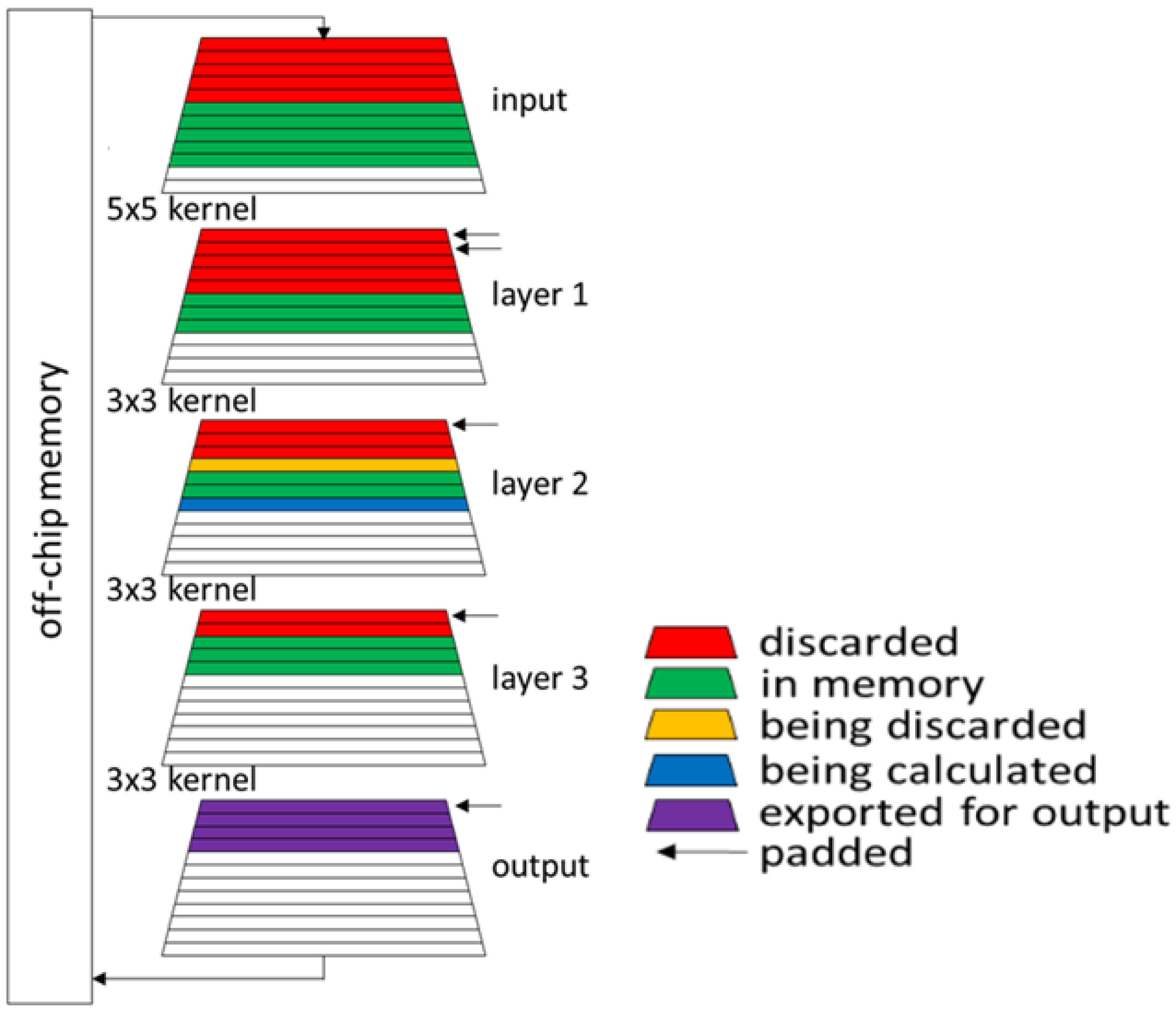
Therefore, the depth-first principle [15,16,17] is presented and illustrated in Figure 3. When one line of an input image is sent from the off-chip memory to the on-chip, this line can be used to compute one line of the first output feature layer. This line can subsequently be used to compute a new line of the second output feature layer, etc. This technique reduces the number of active features as the computation of a new line makes another layer of the same feature map that can be discarded. From each layer, the number of lines that need to be stored is equal to the height of the filter kernel, which is typically 1/3/5. This number is, of course, much lower than the total number of lines in an HD image. Drawbacks are firstly that features from multiple feature maps have to be stored at the same time, but this still leads to major savings for HD images. Secondly, weights from multiple weight tensors need to be stored on-chip at the same time. However, for HD images, weights have much lower memory usage than features. Therefore, depth-first will always be beneficial for HD image-related CNN executions.

In the literature, hardware architectures for depth-first or layer-fused execution are published [16]. However, these hardware architectures are optimized to execute the depth-first principle in straightforward networks. For the benchmarked networks in [16], the reduction in I/O communication due to depth-first goes up to 81×. As mentioned above, stereo-based depth estimation networks are not straightforward, mainly due to the two paths at the beginning of the network. Therefore, this work will present a hardware architecture for a stereo-based depth estimation network that can exploit the benefits of depth-first execution efficiently for multi-path networks and deal efficiently with special layers like concatenation and element-wise operations. This architecture and the corresponding scheduling will be discussed in the next two sections.

3. Hardware Architecture

3.1. Introduction

Figure 4 describes the hierarchical overview of the proposed flexible multi-core processor for stereo-based depth estimation. It is very important to stress that the design is parameterized. This means that compute array sizes and memories can be taken as big as required by the user.

The innermost module is the ‘Architecture’ module, which is the datapath, consisting of all compute and memory blocks. This datapath will be discussed in more detail in the remainder of this section.

The module on top of the ‘Architecture’ module is the ‘FSMOneLine’ module. This module contains the procedure on how to execute one line for the depth-first/layer-fused approach, for one convolutional layer of the network, in combination with stereo-based specific elements like concatenation/addition/multiplication. This module will be discussed in detail in Section 4.

The outermost module is the ‘FSMCompleteNetwork’ module. This module indicates the order in which the computations of one line for one layer need to happen, and therefore performs the actual depth-first execution. A possible order of instructions from this module to ‘FSMOneLine’ might be: line 1 of layer 1, line 2 of layer 1, line 3 of layer 1, line 1 of layer 2, line 4 of layer 1, line 2 of layer 2, etc. As this module is network-dependent, we will not discuss the implementation in this paper. The other two modules are network independent. ‘FSMCompleteNetwork’ needs to give as information to ‘FSMOneLine’: which instruction must be executed (convolutional layer dimensions, other operand like concatenation or not), the address number(s) of the memory/memories where data are located to perform the executions with, and the address number(s) of the memory/memories where resulting data should be stored.

3.2. Overview of the Architecture Datapath

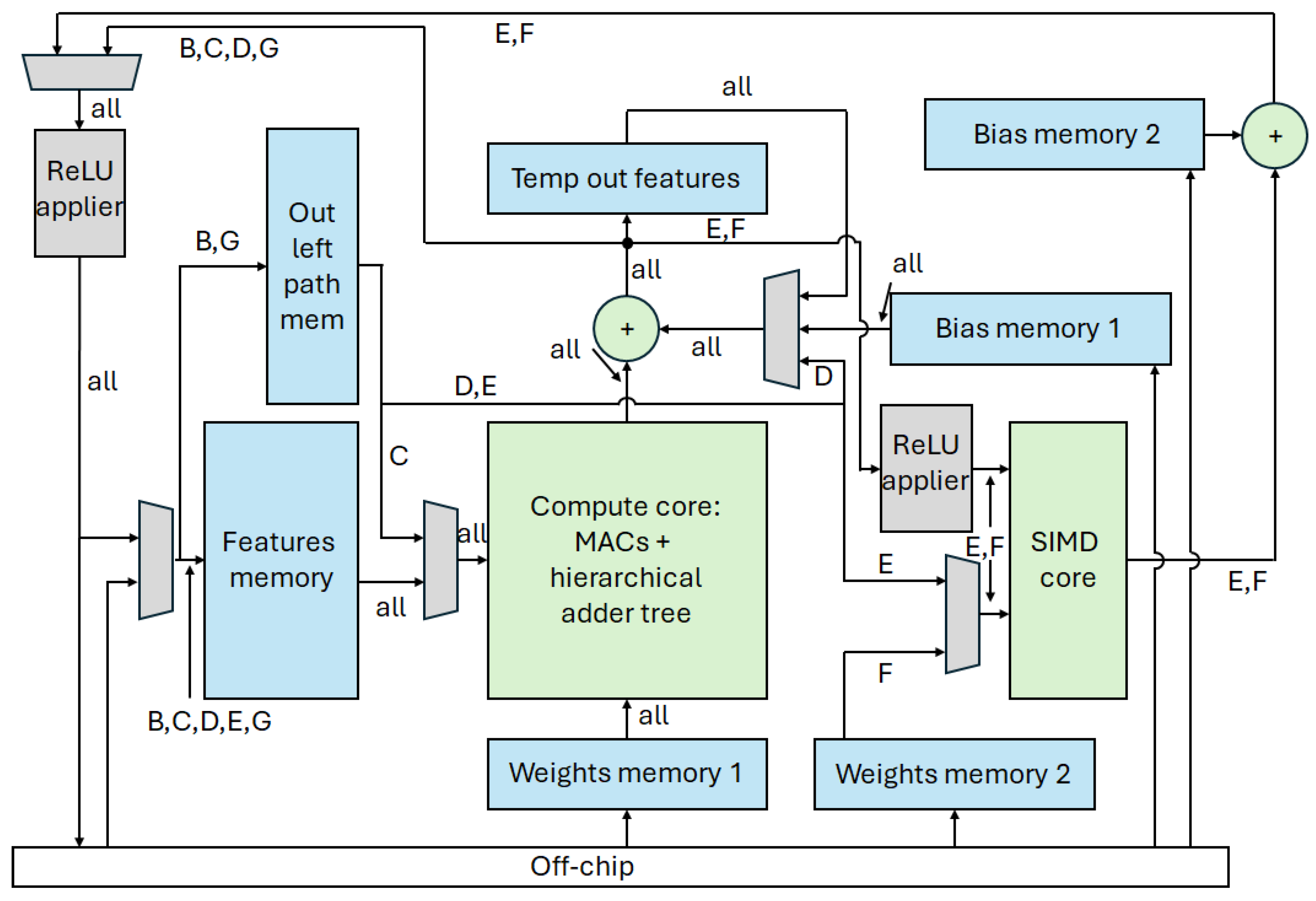
Figure 5 contains the schematic overview of the flexible hardware architecture that will be used to compute stereo-based depth estimation CNNs. The main novelty is the addition of a SIMD secondary core next to the main core. This second core will lead to reduced latency. The architecture also contains six memory blocks. Hence, there is a need for multiplexers to correctly assign data to compute blocks. The next subsections discuss these blocks in more detail, and Section 4 discusses the scheduling of the different layer types on this hardware architecture.

3.3. Compute Core

The main compute core in the middle of Figure 5 will be used to compute most of the convolutional layers. The core contains $N\times N$ multipliers.

A spatial parallelization of $C|K$, where C represents the input channels and K represents the output channels, will be used, as this parallelization ideally supports depth-first execution because one chunk of output data that is computed together is also used as one chunk of input data in the next layer. As can be seen in Figure 6, this means that N input channels of a given input pixel will be broadcast horizontally over the array. There are N hierarchical adder trees, each adding the N products in a given column, coming from N different input channels. Therefore, each column represents a different output channel. The N output channels all belong to the same output pixel.

3.4. SIMD Core

The SIMD Core contains N multipliers, the same as the size of one dimension of the main compute core. This block will be used to compute convolutional layers with a very limited number of output channels and to compute element-wise multiplications, where the two paths of the stereo-based CNN come together.

3.5. Other Adders

Outside these two cores, there are also two rows of N adders. The N adders on top of the main compute core in Figure 5 are needed because the computation of a given output feature will not be done in one clock cycle. Therefore, these adders will be used to add temporary output features with a new sum of N products as delivered by the main compute core. The first time computations for a given output feature are happening, these adders can also be used to add the bias. The adders will also be used to perform element-wise addition where the left and right paths come together.

The N adders at the top right of Figure 5 will be used to add the bias of the layers with a very limited number of output channels.

3.6. ReLU Operator

The two ReLU (rectified linear unit) blocks in Figure 5 both contain N conditional ReLU units. If a ReLU operation has to be applied, a check on the sign bit of the data will take place. In case the data is negative, a 0 will propagate. Elsewhere, the input will propagate. All ReLU operators are conditional, as it can be programmed whether or not the computation (like a convolutional layer) has to be followed by a ReLU.

3.7. Memories

There are seven memory blocks in the architecture of Figure 5. Each has a bandwidth of $N\times R$ bits, where N is based on the dimension of the compute blocks and R is the precision of a word in bits. The number of addresses of each memory is parameterizable and can therefore be adjusted to the (set of) networks that need to be executed. The two memories on the left contain fully computed features. The ‘out left path mem’ memory contains features at the end of the left path, just before an operation to merge the two paths occurs: a concatenation, a multiplication, or an addition. The ‘features memory’ contains all other fully computed features. The ‘temp other features’ memory at the top contains temporal output features that are not yet fully computed and need to be updated further. The other memory blocks contain weights or biases for convolutional layers to be executed on the compute or SIMD core.

4. Scheduling on Hardware

4.1. Introduction

The architecture file describes the modules, i.e., what happens in one clock cycle. Of course, there is also the need for scheduling procedures. This scheduling will make use of a depth-first approach, as discussed above. The proposed solution makes use of a module that will perform the scheduling for the computation of one line of one convolutional layer, in some cases executed in parallel with another operation, like concatenation or element-wise operations. Section 4.2–Section 4.7 discuss in detail how all these operations will be handled. Figure 5 illustrates where data will flow for each of these subsections.

4.2. Stand-Alone Convolutional Layer: Depth-First

To compute one output line of width $OX$, with K output channels and C input channels, using a $FX\times FY$ filter kernel and the $C|K$ spatial unrolling, the temporal mapping of Algorithm 1 will be used.

Algorithm 1 Scheduling for Section 4.2

1: for k in range(K/N) do 2:     for c in range(C/N) do 3:         for fx in range(FX) do 4:            for fy in range(FY) do 5:                for ox in range(OX) do 6:                    parfor c: 7:                    parfor k: 8:                    O[][][] += I[][][]*W[][][][] 9:                end for 10:            end for 11:         end for 12:     end for 13: end for

Here, N is still the number of rows or columns of the main compute core. Note that there is no need for a ‘for oy’ loop as we are only computing only line line of the convolutional layer. The ‘for ox’ loop is the most inner for loop. This is done to make sure our weight can be kept stationary over $OX$ clock cycles. $N^2$ weights are needed in parallel, where we are only handling N input features and N output features. Therefore, the weights are the most interesting to keep stationary. The ‘for k’ loop is placed at the top. This is to minimize the number of temporal, not-yet-final output features of the convolutional layer, hereby optimizing the size of the ‘temp out features’ memory. The order of the three other for loops, which are situated in the middle, doesn’t impact memory requirements and is therefore picked arbitrarily.

Figure 5 illustrates how the data for this execution flows. Features will always come from the ‘features memory’ as this mode will never be activated with the outputs of the left path as input (see Section 4.4). Weights and bias memory 1 are activated. After the first time temporal data are generated for a given output pixel, the adder row indicated in red (on top of the main compute core) will be used to add biases that come from the bias memory. Hereafter, the multiplexer at the input of this adder row will make sure the temporal output features are updated with the new results, coming from the main compute core. When the output features are done, they are sent from the adder row immediately to the ReLU applier and from here to the correct features memory (output of left path or not) or the off-chip memory (external world) in case this is required by the optimal network scheduling.

Figure 7 shows the memory structure of the features memory. For efficient, correct, and network-independent execution of the ‘FSMOneLine’ module, it is important that the structure of data distribution in the memory is always the same. The module needs to get as input the first address of the features layer from which it needs to read the input data, and the first address that corresponds to where the output row of the convolutional layer needs to be written. One additional input is the ‘pointer’ that indicates which of the $FX$ rows in memory is currently the top one. In other words, the memory will be a circular buffer. As discussed before, depth-first execution allows us to discard data that is not needed anymore for further computations and replace it with new features. At the time of computing the first output row of the first convolutional layer, the FX top rows from the input features layer are placed in order in the features memory. However, after discarding the top row of the input features layer and replacing it in memory with row $FX+1$, the data at the position of ‘row 2’ in the memory belongs to the highest row that is currently in the memory. Therefore, the pointer should now point to row 2. This means that ‘FSMOneLine’ can operate in a network-independent and scheduling-independent way.

4.3. Concatenation of Stereo Paths

This subsection describes the scheduling for computing one line of one convolutional layer, which is preceded by a concatenation operation of the outputs of the left and right paths of the network. The main difference with the scheduling in Section 4.2 is the fact that half of the inputs have to come from the ‘out left path mem’ and the other half from the ‘features memory’ (for the right path’s outputs). The multiplexer in front of the compute core arranges this. Outputs only have two instead of three possible destinations, as results are by definition not the output of the left path anymore. The updated for loop implementation is given in Algorithm 2.

4.4. Addition of Stereo Paths

This subsection describes the scheduling for computing one line of the final convolutional layer of the right path, fused with the element-wise addition of the left and right path features. The working principle is very similar to the one presented in Section 4.2. The main difference is that features from ‘out left path mem’ are now used instead of biases. A network with this kind of structure can always be rewritten to a network where the last convolutional layer of the right path has no bias.

4.5. Multiplication of Stereo Paths

This subsection describes the scheduling for computing one line of the final convolutional layer of the right path, fused with the element-wise addition of the left and right path features. This is the first scheduling where the SIMD Core will be used. The computation of the one line of the convolutional layer is done similar to Section 4.2. Although the output is not immediately sent to the left ReLU applier and memory, but to the ReLU applier in front of the SIMD Core. Here, the element-wise multiplication with the features from the ‘out left path mem’ memory happens, before writing back the data that will be the inputs of the next convolutional layer.

Algorithm 2 Scheduling for Section 4.4

1: for k in range(K/N) do 2:     for c in range(Cright/N) do 3:         for fx in range(FX) do 4:            for fy in range(FY) do 5:                for ox in range(OX) do 6:                    parfor c: 7:                    parfor k: 8:                    O[][][] += I[][][]*W[][][][] 9:                end for 10:            end for 11:         end for 12:     end for 13:     for c in range(Cleft/N) do 14:         for fx in range(FX) do 15:            for fy in range(FY) do 16:                for ox in range(OX) do 17:                    parfor c: 18:                    parfor k: 19:                    O[][][] += I[][][]*W[][][][] 20:                end for 21:            end for 22:         end for 23:     end for 24: end for

4.6. Final Convolutional Layers of Network

This subsection describes the scheduling for computing one line of the final two convolutional layers of the network. The computation of these two lines will happen in parallel. Typically, the last layer of a convolutional neural network contains a very limited number of output channels (mostly 1), and a 1 × 1 kernel, as in [18]. Therefore, the utilisation of the main compute core would be very low when evaluating this convolutional layer, as only 1 out of the N columns would be used. In this way, it is better to use the SIMD core to be able to immediately consume the output of the penultimate convolutional layer to compute the outputs of the final convolutional layer. The latency of this final layer is completely hidden in this way and can actually be counted as 0.

4.7. First Convolutional Layer of Network

The first layer of a convolutional network would also not execute very efficiently on the main compute core with $C|K$ spatial mapping, as the number of input channels is typically very low (typically RGB or greyscale image as input). Therefore, for these types of layers, the spatial mapping can be changed to $\left(C\right|FX\left|FY\right)|K$. As $FX$ and $FY$ are typically not 1 for these layers, more rows of the compute core can be used, so utilisation will increase and latency will decrease. By duplicating input features and reformulating the weight tensors, no changes to the datapath are needed in comparison with the regular $C|K$ spatial mapping from Section 4.2.

5. Case Study

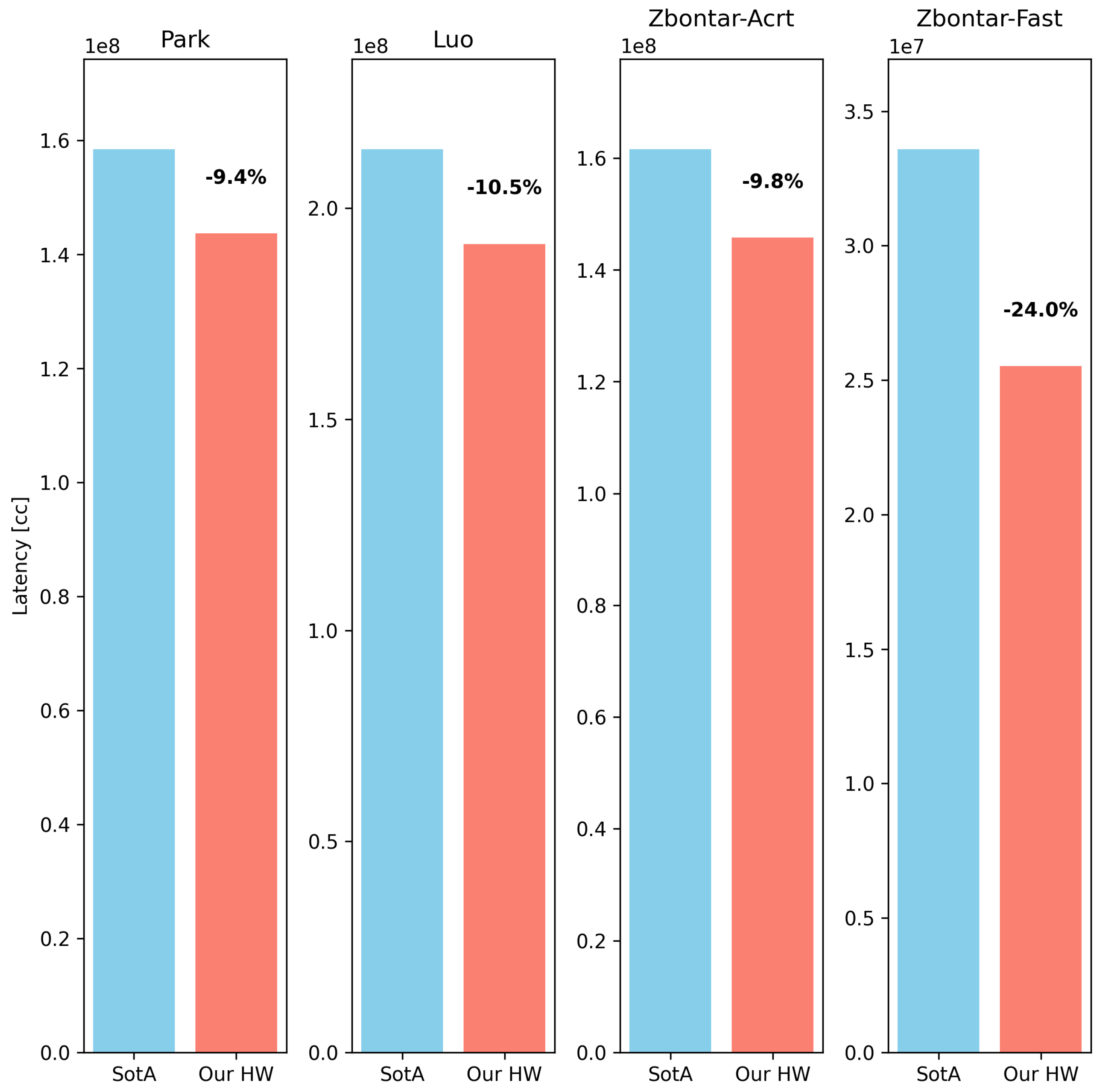
As a case study, we will discuss four networks: the network defined by Park [8], the network defined by Luo [9] and the two networks proposed by Zbontar [18]. They present a fast and accurate network. All these four have the structure as shown in Figure 2. We will compare the latency when using the standard depth-first approach (only schedule B from Section 4) with the presented hardware architecture, supporting all schedules mentioned in Section 4. We will vary the value of N from 32 to 64, therefore simulating an architecture with a main core of size $32\times 32$ and an architecture with a main core of $64\times 64$. This investigation seeks to answer two primary questions:

• Which network architecture benefits the most from the proposed design?
• How does the size of the main core array influence the performance?

The results of the experiments can be found in Figure 8 and Figure 9. The latency percentages are for the evaluation of the complete networks. These networks are interpreted as an enumeration of neural layers. Each layer is split in OY ‘computation nodes’ that each compute one line. That one line is computed using the schedulings as discussed in Section 4. Based on the experimental results, we now generalize our findings to address the two research questions. The proposed architecture yields the greatest performance benefits for the fast version of Zbontar, which is a relatively compact neural network, with a limited number of layers and feature channels. In such cases, the flexible scheduling and efficient resource utilization enabled by our design translate into substantial latency reductions. Above, the architecture has more benefits in terms of latency when the combination method between the two paths is a multiplication or addition operation instead of a concatenation, for which no computations are needed but only a smart memory structure. For the accurate version of Zbontar, the proposed architecture also takes profit of the fact that the last convolutional layer has one output channel. The SIMD core can there be used to perform this convolutional layer while the main compute core performs the penultimate layer. Moreover, the latency improvements become more pronounced as the size of the main processing core increases. This trend aligns with ongoing developments in hardware design, where larger and more capable processing arrays are becoming increasingly prevalent. One might now ask the question: why do we spend these compute elements on a second core (the SIMD core)? In Figure 8 and Figure 9, we compare two architectures with a different number of MACs. Wouldn’t it be more efficient to spend these additional resources to make the main core bigger, e.g., a $33\times 33$ main core array for the first case and a $65\times 65$ main core array for the second case? The answer to that question is a clear ‘no’. The input and output channels are spatially parallelized over the columns and rows of the main core array. Let us take the example of the fast network, with mostly layers with 64 channels. A spatial parallelization of 32 channels leads to the need for 2 temporal iterations over the channels (64/32). A spatial parallelization of 33 channels would also lead to the need for 2 temporal iterations over the channels (64/33). Therefore, increasing the $32\times 32$ array to a $33\times 33$ array would literally lead to the reduction of 0 clock cycles due to the mismatch in the number of channels and spatial parallelization over the channels. Note that the decrease in latency is greater than the increase in the number of MACs. When adding an additional SIMD core with 32 multipliers besides a $32\times 32$ main core, latency decreases by 5.7% and 13.5%, respectively for the two networks, where the number of MACs increases by 3.1%. This means that besides the latency, the utilization is also better. The effect on utilization is even greater for the case where the main core has a size $64\times 64$, as latency decreases there with 9.8% and 24%, for an increase of only 1.6% in compute resources.

For reproducibility of this case study, we refer to the detailed breakdown analysis on the mentioned Github page.

6. Conclusions

In this work, we propose a flexible multi-core hardware architecture specifically designed to support stereo-based depth estimation convolutional neural networks (CNNs). Traditional CNN implementations processing high-definition images often face significant challenges related to memory bandwidth and I/O demands, resulting in increased energy consumption and area costs. Although recent depth-first execution strategies help alleviate these issues by consuming intermediate features immediately after computation, they are ill-suited to the dual-path structures inherent to stereo-based networks. To overcome this limitation, we developed an architecture that integrates the advantages of depth-first processing with specialized support for the complex layer interconnections typical of stereo-based CNNs. Our design is also flexible, as it is independent of the network topology and execution schedule. Through a detailed case study, we demonstrate that our architecture delivers the greatest performance gains for compact networks with limited depth and channel width. Furthermore, we show that latency improvements scale with the size of the processing core, highlighting the architecture’s suitability for deployment on modern hardware platforms with increasing computational density. Compared to state-of-the-art depth-first implementations without stereo-specific optimizations, our architecture achieves a latency reduction of up to 24%. All used networks are not extremely recent (however all of them less than 10 years old, so also not prehistorical), but they are still useful in practice, just like the even older ResNet for example. More recent networks typically contain more and more types of features like softmax for example. The authors work on a hardware extension to also be able to deal with these.

References

1. Ponrani, M.A.; Ezhilarasi, P.; Rajeshkannan, S. Robust stereo depth estimation in autonomous vehicle applications by the integration of planar constraints using ghost residual attention networks. Signal Image Video Process. 2025, 19, 1163. [Google Scholar] [CrossRef]
2. Kemsaram, N.; Das, A.; Dubbelman, G. A stereo perception framework for autonomous vehicles. In Proceedings of the 2020 IEEE 91st Vehicular Technology Conference (VTC2020-Spring), Antwerp, Belgium, 25–28 May 2020; pp. 1–6. [Google Scholar]
3. Xu, Y.; Chen, S.; Yang, X.; Xiang, Y.; Yu, J.; Ding, W.; Wang, J.; Wang, Y. Efficient and Hardware-Friendly Online Adaptation for Deep Stereo Depth Estimation on Embedded Robots. IEEE Robot. Autom. Lett. 2025, 10, 4308–4315. [Google Scholar] [CrossRef]
4. Tian, C.; Pan, W.; Wang, Z.; Mao, M.; Zhang, G.; Bao, H.; Tan, P.; Cui, Z. Dps-net: Deep polarimetric stereo depth estimation. In Proceedings of the IEEE/CVF International Conference on Computer Vision, Paris, France, 2–3 October 2023; pp. 3569–3579. [Google Scholar]
5. Laga, H.; Jospin, L.V.; Boussaid, F.; Bennamoun, M. A survey on deep learning techniques for stereo-based depth estimation. IEEE Trans. Pattern Anal. Mach. Intell. 2020, 44, 1738–1764. [Google Scholar] [CrossRef] [PubMed]
6. Smolyanskiy, N.; Kamenev, A.; Birchfield, S. On the importance of stereo for accurate depth estimation: An efficient semi-supervised deep neural network approach. In Proceedings of the IEEE Conference on Computer Vision and Pattern Recognition Workshops, Seattle, WA, USA, 14–19 June 2020; pp. 1007–1015. [Google Scholar]
7. Xiang, J.; Wang, Y.; An, L.; Liu, H.; Wang, Z.; Liu, J. Visual attention-based self-supervised absolute depth estimation using geometric priors in autonomous driving. IEEE Robot. Autom. Lett. 2022, 7, 11998–12005. [Google Scholar] [CrossRef]
8. Park, H.; Lee, K.M. Look wider to match image patches with convolutional neural networks. IEEE Signal Process. Lett. 2016, 24, 1788–1792. [Google Scholar] [CrossRef]
9. Luo, W.; Schwing, A.G.; Urtasun, R. Efficient deep learning for stereo matching. In Proceedings of the IEEE Conference on Computer Vision and Pattern Recognition, Las Vegas, NV, USA, 27–30 June 2016; pp. 5695–5703. [Google Scholar]
10. Ye, X.; Li, J.; Wang, H.; Huang, H.; Zhang, X. Efficient stereo matching leveraging deep local and context information. IEEE Access 2017, 5, 18745–18755. [Google Scholar] [CrossRef]
11. Satushe, V.; Vyas, V. Use of CNNs for Estimating Depth from Stereo Images. In Proceedings of the International Conference on Smart Computing and Communication, Bali, Indonesia, 25–27 July 2024; Springer Nature: Singapore, 2024; pp. 45–58. [Google Scholar]
12. Aguilera, C.A.; Aguilera, C.; Navarro, C.A.; Sappa, A.D. Fast CNN stereo depth estimation through embedded GPU devices. Sensors 2020, 20, 3249. [Google Scholar] [CrossRef] [PubMed]
13. Wang, Z.; Zou, Y.; Lv, J.; Cao, Y.; Yu, H. Lightweight Self-Supervised Monocular Depth Estimation Through CNN and Transformer Integration. IEEE Access 2024, 12, 167934–167943. [Google Scholar] [CrossRef]
14. Zhang, N.; Nex, F.; Vosselman, G.; Kerle, N. Lite-mono: A lightweight cnn and transformer architecture for self-supervised monocular depth estimation. In Proceedings of the IEEE/CVF Conference on Computer Vision and Pattern Recognition, Vancouver, BC, Canada, 17–24 June 2023; pp. 18537–18546. [Google Scholar]
15. Goetschalckx, K.; Verhelst, M. Breaking high-resolution CNN bandwidth barriers with enhanced depth-first execution. IEEE J. Emerg. Sel. Top. Circuits Syst. 2019, 9, 323–331. [Google Scholar] [CrossRef]
16. Colleman, S.; Verhelst, M. High-utilization, high-flexibility depth-first CNN coprocessor for image pixel processing on FPGA. IEEE Trans. Very Large Scale Integr. (VLSI) Syst. 2021, 29, 461–471. [Google Scholar] [CrossRef]
17. Symons, A.; Mei, L.; Colleman, S.; Houshm, P.; Karl, S.; Verhelst, M. Stream: A Modeling Framework for Fine-grained Layer Fusion on Multi-core DNN Accelerators. In Proceedings of the 2023 IEEE International Symposium on Performance Analysis of Systems and Software (ISPASS), Raleigh, NC, USA, 23–25 April 2023; pp. 355–357. [Google Scholar]
18. Žbontar, J.; LeCun, Y. Stereo matching by training a convolutional neural network to compare image patches. J. Mach. Learn. Res. 2016, 17, 1–32. [Google Scholar]
19. Zbontar, J.; LeCun, Y. Computing the stereo matching cost with a convolutional neural network. In Proceedings of the IEEE Conference on Computer Vision and Pattern Recognition, Boston, MA, USA, 7–12 June 2015; pp. 1592–1599. [Google Scholar]
20. Dosovitskiy, A.; Fischer, P.; Ilg, E.; Hausser, P.; Hazirbas, C.; Golkov, V.; van der Smagt, P.; Cremers, D.; Brox, T. Flownet: Learning optical flow with convolutional networks. In Proceedings of the IEEE International Conference on Computer Vision, Santiago, Chile, 7–13 December 2015; pp. 2758–2766. [Google Scholar]
Figure 1. Illustration of stereo-based depth estimation.
Electronics 14 04425 g001
Figure 2. Concept of stereo-based depth estimation networks: left and right image branches that merge mid-way.
Electronics 14 04425 g002
Figure 3. Concept of depth-first principle, based on [16].
Electronics 14 04425 g003
Figure 4. Hierarchical overview of the modules.
Electronics 14 04425 g004
Figure 5. Schematic overview of our hardware architecture. Computation blocks are indicated in green, memories in blue, and data handling blocks like multiplexers in grey. The letters next to the data buses indicate for which dataflows, described in Section 4.2Section 4.7, that particular data bus is used: B = Stand-Alone Convolutional Layer, C = Concatenation of Stereo Paths, D = Addition of Stereo Paths, E = Multiplication of Stereo Paths, F = Final Convolutional Layers of Network, G = First Convolutional Layer of Network.
Electronics 14 04425 g005
Figure 6. Main compute core with N = 4 . Features from 4 input channels are broadcast horizontally over the array and column-wise added for each of the 4 output channels.
Electronics 14 04425 g006
Figure 7. Memory structure of features memory.
Electronics 14 04425 g007
Figure 8. Impact of proposed architecture with N = 32 on the four networks under study.
Electronics 14 04425 g008
Figure 9. Impact of proposed architecture with N = 64 on the four networks under study.
Electronics 14 04425 g009
Disclaimer/Publisher’s Note: The statements, opinions and data contained in all publications are solely those of the individual author(s) and contributor(s) and not of MDPI and/or the editor(s). MDPI and/or the editor(s) disclaim responsibility for any injury to people or property resulting from any ideas, methods, instructions or products referred to in the content.