Abstract
The increasing demand for data utilization has renewed attention to the trade-off between privacy protection and data utility, particularly concerning pseudonymized datasets. Traditional methods for evaluating re-identification risk and utility often rely on fragmented and incompatible metrics, complicating the assessment of the overall effectiveness of pseudonymization strategies. This study proposes a novel quantitative metric—Relative Utility–Threat (RUT)—which enables the integrated evaluation of safety (privacy) and utility in pseudonymized data. Our method transforms various risk and utility metrics into a unified probabilistic scale (0–1), facilitating standardized and interpretable comparisons. Through scenario-based analyses using synthetic datasets that reflect different data distributions (balanced, skewed, and sparse), we demonstrate how variations in pseudonymization intensity influence both privacy and utility. The results indicate that certain data characteristics significantly affect the balance between protection and usability. This approach relies on simple, lightweight computations—scanning the data once, grouping similar records, and comparing their distributions. Because these operations naturally parallelize in distributed environments such as Spark, the proposed framework can efficiently scale to large pseudonymized datasets.
1. Introduction
In contemporary society, the importance of data continues to grow, playing a central role in decision-making and analysis across various fields. Concurrently, increasing concerns and stricter regulations regarding personal information protection have created an urgent demand for secure data utilization methods. In this context, pseudonymization and anonymization have emerged as key approaches to achieving the dual goals of privacy protection and data utility.
Pseudonymization aims to preserve as much of the original data’s utility as possible while reducing re-identification risk. By transforming sensitive information to prevent direct exposure, it enables users to understand and use the data’s meaning while lowering the likelihood of individual identification. In contrast, anonymization seeks to eliminate the possibility of re-identification entirely, even in the presence of external data linkage or adversarial inference attacks. This stronger protection often comes at the expense of accuracy and granularity in the data available for analysis.
This study proposes a new set of quantitative metrics designed to evaluate safety, utility, and the balance between the two in pseudonymized datasets. Conventional privacy-preserving techniques have primarily focused on reducing re-identification risk, but these methods frequently degrade data utility, limiting practical use. To address this issue, we develop metrics that enable the simultaneous assessment of privacy protection and utility in pseudonymized data.
The proposed metrics quantify re-identification risk while also measuring information loss and similarity to the original data. This dual evaluation allows data controllers to easily assess levels of safety and utility, enabling informed decisions about adjusting the degree of pseudonymization or implementing additional safeguards. Notably, the metrics are expressed on a probabilistic scale ranging from 0 to 1, offering an intuitive and interpretable means of understanding the trade-off between protection and usability.
Beyond internal evaluation, this study introduces an approach to measuring linkage risks between pseudonymized datasets and external data, identifying potential re-identification vulnerabilities in real-world scenarios. By incorporating such interactions into the evaluation, the proposed method provides a comprehensive framework for assessing data safety. Scenario-based visualization further demonstrates that the balance between privacy and utility varies considerably depending on data distribution characteristics, even when the same pseudonymization intensity is applied.
Therefore, this study offers a novel evaluation framework to ensure both safety and usability in pseudonymized datasets. The proposed approach provides practical support for balancing data protection and utility in real-world applications, contributing to enhanced privacy safeguards while maximizing the potential for data-driven insights.
2. Background and Related Work
2.1. Data Privacy Protection Techniques
As the importance of data continues to grow, data-driven decision-making and analysis have become essential across various domains. However, the increase in data utilization has also heightened concerns and demands for personal data protection [1,2,3,4,5,6,7,8,9]. In this context, diverse data privacy protection techniques have been developed to ensure security while maintaining usability, with anonymization and pseudonymization being the most representative approaches.
Anonymization refers to transforming data so that individuals can no longer be identified, completely eliminating the possibility of re-identification. Prominent anonymization techniques include k-anonymity [10,11,12,13], l-diversity [14], and t-closeness [15]. k-anonymity ensures that each record in a dataset shares identical attributes with at least k other records, making individual identification more difficult. By creating data groups with a similarity level above a predefined threshold k, this method reduces the likelihood that an attacker can re-identify a specific individual. l-diversity was introduced to address k-anonymity’s limitations by requiring diversity of sensitive attributes within each group, ensuring that the distribution of sensitive information maintains a minimum level of variety to enhance confidentiality. t-closeness further extends this protection by ensuring that the distribution of sensitive attributes within a group is similar to that of the overall dataset, preventing the inference of sensitive information about individuals and complementing l-diversity by reducing the risk of attribute disclosure. These anonymization methods aim to minimize re-identification risks and enhance privacy protection. However, they often compromise utility, as excessive generalization or removal of critical details can undermine the reliability of analyses. Research has recently expanded to include privacy-enhancing technologies [16], synthetic data generation [17,18,19,20,21,22,23,24], and differential privacy approaches [25,26,27,28,29].
Pseudonymization, by contrast, modifies only certain identifiers so that individuals are not readily identifiable while still allowing for re-identification under specific conditions—such as repeated analyses in time-series datasets. Pseudonymized data retains more of the original semantic content, offering significant advantages for analysis and practical applications. Although it does not guarantee complete elimination of re-identification risks, pseudonymization maximizes data usability while making direct identification difficult without external datasets. Consequently, pseudonymized data has become widely applicable in practice, including research, analytics, and marketing. The primary goal of pseudonymization is to minimize the risk of re-identification. Unlike anonymization, which aims to eliminate such risk almost entirely, pseudonymization preserves portions of the original data, thereby maintaining its utility.
Both anonymization and pseudonymization seek to protect data privacy, but they differ significantly in approach and outcome. Anonymization aims to eliminate any possibility of re-identification, often at the expense of utility, whereas pseudonymization seeks to balance protection with usability by preserving partial information. Thus, anonymized data is virtually free of re-identification risk but often less useful, while pseudonymized data maintains higher utility at the cost of residual risk [30,31,32,33].
2.2. Need for Metrics to Evaluate Re-Identification Risk and Utility
Since pseudonymized data does not completely eliminate the possibility of re-identification, there remains a risk that such data can be re-identified when combined with external information. For this reason, it is essential for data controllers to quantitatively evaluate the degree of re-identification risk present in pseudonymized datasets. Such evaluations serve as critical evidence for determining whether the data is sufficiently protected and whether additional safeguards are necessary.
Traditional methods for assessing re-identification risk have largely focused on anonymized datasets, typically evaluating whether specific thresholds of k-anonymity are met or whether sufficient diversity exists in sensitive attributes. However, these approaches are not fully suited for pseudonymized datasets, which inherently retain some degree of re-identification risk. Therefore, more fine-grained and quantitative metrics are needed to evaluate re-identification risk in pseudonymized data.
When privacy-preserving techniques are applied, the structure or values of the data are inevitably altered. These modifications directly affect data utility, making it crucial to assess whether the transformed data can still be meaningfully analyzed and produce reliable results. To this end, information loss and original similarity are commonly used metrics. Information loss measures the extent to which information is degraded through transformation, often by evaluating how much attributes are generalized or altered. Similarity metrics, in contrast, assess the structural and pattern-based resemblance between pseudonymized and original data, providing insights into whether the transformed data can yield analysis results consistent with the original dataset.
A fundamental trade-off exists between privacy protection and data utility. Stronger protection measures reduce the risk of re-identification but also diminish utility, while maximizing utility inevitably entails lowering the level of privacy protection. Most previous research has focused on either privacy or utility in isolation, with insufficient emphasis on integrated evaluation. This gap motivates the present study, which proposes a new metric designed to capture and balance the trade-off between privacy and utility, enabling a more comprehensive assessment.
2.3. Comparison with Previous Studies
Existing approaches to evaluating re-identification risk have primarily relied on k-anonymity-based models. These models ensure that every record in a dataset shares its attributes with at least k other records, thereby lowering the likelihood of identifying a specific individual. However, this approach often conflicts with the requirements of pseudonymization, which must maintain continuity and consistency with the original data. Since pseudonymization is applied under constraints that preserve analytical and operational usability, traditional privacy models such as k-anonymity are insufficient for fully capturing the re-identification risk in pseudonymized datasets.
Previous studies have also proposed a variety of quantitative measures for data utility, including information loss, generalization loss, and data similarity. However, these metrics differ in methodology and interpretation, limiting their effectiveness for comprehensive and consistent evaluation. For instance, generalization loss is useful for numerical attributes expressed as ranges but is less applicable to complex data types such as categorical or time-series data. Consequently, there has been growing demand for new metrics capable of integrating utility into a single interpretable index. However, relatively few studies have considered the trade-off between re-identification risk and utility; most have focused only on privacy, treating utility as a secondary, qualitatively observed outcome under certain protection conditions. This study addresses these shortcomings by quantifying both re-identification risk and data utility and integrating them into a unified balance metric. This enables more systematic and objective comparisons and provides a decision-making framework for policymakers.
Specifically, this study builds on and improves upon the limitations of prior work. For example, Ponte [34] proposed an information-theoretic framework for measuring the identifiability of individual records but did not account for dataset-level utility or balance. Sondeck and Laurent [35] empirically assessed re-identification risk in real pseudonymization environments but did not examine data utility. Shlomo and Skinner [36] established theoretical models of re-identification for statistical microdata, while Xia et al. [37] applied GAN-based adversarial modeling to quantify re-identification risks in healthcare datasets. However, these studies share a common limitation: they either focus solely on re-identification risk or omit analysis of the risk–utility balance.
In terms of data utility assessment, existing approaches have largely relied on single-dimension measures such as information loss or similarity. These vary in applicability depending on data characteristics and processing methods, making consistent comparisons across diverse data environments difficult.
By contrast, the present study provides a distinct contribution by offering a unified evaluation framework for pseudonymized data that simultaneously quantifies realistic re-identification risk and data utility, integrating them into the proposed Relative Utility–Threat (RUT) metric. This framework enables objective comparisons of data protection and usability, directly supporting practical policy and implementation decisions. Moreover, through scenario-based analysis reflecting different distribution characteristics (balanced, skewed, and sparse datasets), the study empirically validates how structural properties of data affect the privacy-utility balance—demonstrating practical applicability beyond the scope of prior research.
2.4. Distinctive Contributions of This Study
This study proposes novel metrics to quantitatively evaluate the safety, utility, and balance of pseudonymized datasets. While previous research has tended to focus either on anonymized data or has evaluated only re-identification risk or data utility in isolation, the present work emphasizes a comprehensive assessment of the trade-off between privacy protection and usability. The main points of distinction are as follows:
- Pseudonymization-Specific Metrics: Unlike anonymization, pseudonymization allows for a certain level of re-identification risk. Therefore, specialized metrics are required to quantify this risk in practical settings. This study introduces new measures tailored to pseudonymized datasets, including metrics for re-identification risk, external linkage vulnerability, and data utility.
- Balanced Evaluation of Safety and Utility: Previous studies lacked robust methods to quantify the trade-off between privacy and utility. This study addresses this gap by proposing a new metric that directly measures the balance between safety and usability. With this, data processors are equipped with clearer criteria to optimize decisions on data protection while still enabling meaningful utilization.
- Normalized, Intuitive Quantification: All proposed metrics are expressed as normalized probability values between 0 and 1, allowing for straightforward interpretation. This design enables data processors to intuitively grasp each metric and efficiently evaluate both safety and utility. The approach not only simplifies decision-making but also supports the development of effective data management strategies grounded in transparent and easily interpretable results.
3. Proposed Quantitative Evaluation Metrics for Safety, Utility, and Their Balance
3.1. Safety Metric—Re-Identification Risk Score
The safety metric quantifies the probability that pseudonymized data may be re-identified. In other words, if individual records in a pseudonymized dataset are unique or highly similar to only a few other records, the likelihood of re-identification increases. This risk is expressed as the re-identification risk score, which enables the quantification and comparison of re-identification probabilities across datasets. In contrast, this concept does not apply to anonymized data, as the goal of anonymization is to completely eliminate re-identification risk. In principle, if anonymization is perfectly implemented, the probability of re-identification should be zero. The measurement procedure for this metric is as follows (see Table 1):

Table 1.
Safety metric—Calculation method for the re-identification risk score.
[Step 1] For a given dataset, calculate the probability of re-identification for each record, denoted as P(i).
[Step 2] Take the average of the re-identification probabilities (P(i)) from Step 1 across all records, or compute a weighted average by assigning weights according to the sensitivity of each attribute. This yields the overall re-identification risk probability of the dataset, R_internal_risk.
[Step 3] Calculate the probability of external data linkage, R_external_risk. This can be derived using one or a combination of the following approaches: a probability-based method, a correlation-based method, or a unique attribute-combination method. The results may be averaged or weighted depending on the context.
[Step 4] Integrate the results of Steps 2 and 3 to compute the overall re-identification risk (R). This can be achieved through (a) simple addition, (b) weighted averaging, or (c) taking the maximum value between R_internal_risk and R_external_risk. The resulting score is normalized to a probabilistic scale ranging from 0 to 1, where R = 0 indicates no risk of re-identification, and R = 1 indicates a very high likelihood of re-identification.
The detailed calculation methods for each step are as follows:
- Calculation of Re-Identification Probability P(i) for Each Record in Dataset
This metric quantifies the likelihood that an individual record can be re-identified under specific conditions. It assesses how closely the attributes of a given record may match external datasets, thus quantifying re-identification risk. In pseudonymized data, even if certain attributes are transformed, the possibility of re-identification under particular conditions still exists. Therefore, assessing the re-identification probability at the record level is crucial for risk evaluation. In contrast, anonymization aims to eliminate re-identification risk entirely, rendering the calculation of record-level probabilities meaningless.
Let the equivalence class size for record be
where is the attribute set used for risk assessment. We define the re-identification probability of record i as
The specific choice of is instantiated per experiment; see Section 4.2 and Table 7.
- Calculation of Dataset-Wide Re-Identification Probability, R_internal_risk
The overall risk for the dataset is obtained by averaging the record-level probabilities or by applying weights to account for the sensitivity of certain attributes.
where N denotes the total number of records in the dataset, and P(i) refers to the re-identification probability of record i.
- External Data Linkage Probability, R_external_risk
This metric assesses the probability that pseudonymized data may be re-identified when linked with external datasets. The evaluation considers multiple factors and quantifies the risk, particularly by measuring correlations between internal attributes and external data sources. R_external_risk can be computed using one of the following approaches—or by combining them through averaging or weighted averaging: probability-based, correlation-based, and unique attribute-combination approaches. Since pseudonymized data retains some degree of identifiability, external linkage introduces additional risk, making this evaluation essential for determining whether supplementary safeguards or risk-mitigation strategies are needed. In contrast, anonymized data should, by definition, remain non-identifiable even when combined with external datasets, making such linkage risk assessment unnecessary in that context. The detailed approaches for computing R_external_risk are introduced in the following section.
- Probability-Based Approach
This method evaluates the likelihood of re-identification based on how unique or rare certain attribute values are in external datasets.
- ①
- Attribute-Matching Probability Calculation
First, the frequency distribution of specific attributes (e.g., age, postal code, gender) is computed in both the pseudonymized dataset and the external dataset. The attribute-matching probability is derived from these frequencies. For example, if 10% of the pseudonymized dataset contains a particular postal code and the same postal code accounts for 5% of the external dataset, the matching probability for that attribute is 0.1 × 0.05 = 0.005.
- ②
- Overall Matching Probability Calculation
The overall probability of matching across multiple attributes is calculated as the product of the individual attribute-matching probabilities. For example, if attributes A and B have matching probabilities of P(A) and P(B), the combined probability is P(A) × P(B).
- ③
- Re-identification Risk Evaluation
A higher overall matching probability indicates a greater likelihood of re-identification, while a lower value suggests reduced risk. By considering combinations of multiple attributes, the aggregate likelihood that a record can be matched to external data is quantified as a re-identification risk score.
- Correlation-Based Approach
This method evaluates linkage potential by analyzing correlations between attributes in both pseudonymized and external datasets.
- ①
- Calculation Of Attribute Correlations
Correlation coefficients are computed between corresponding attributes in the pseudonymized dataset and the external dataset. Pearson’s correlation coefficient or Spearman’s rank correlation coefficient is typically applied. A higher correlation coefficient indicates a stronger association between datasets and, thus, greater linkage potential.
- ②
- Derivation Of Linkage Score
Linkage scores are obtained from the correlation coefficients of each attribute. These can be aggregated as a simple average or as a weighted average when different attributes are assigned varying importance. The resulting score is then used to evaluate overall re-identification risk.
- Unique Attribute-Combination Approach
This method assesses re-identification risk based on whether unique combinations of attributes can be easily matched to external datasets.
- ①
- Identification Of Unique Attribute Combinations
Unique attribute combinations (e.g., gender, age, and postal code) are identified within the pseudonymized dataset. If such combinations are rare, they may serve as potential identifiers. The existence of similar combinations in the external datasets is then examined.
- ②
- Evaluation Of Linkage Potential
The probability that unique combinations in the pseudonymized dataset appear in external datasets is calculated. If such combinations are extremely rare in external data, they pose a higher re-identification risk. Based on these frequencies, re-identification risk scores are derived to reflect the vulnerability associated with unique combinations.
In summary, high re-identification risk scores arise when pseudonymized and external datasets share attributes with high matching probabilities, strong correlations, or rare unique combinations. In particular, the presence of unique attribute combinations makes it easier to identify specific individuals. Conversely, low scores indicate weaker matches, lower correlations, and reduced linkage potential, signifying stronger protection of pseudonymized data. These quantitative approaches provide a structured way to express linkage risk and support the decision-making process for applying stronger pseudonymization or introducing supplementary safeguards when necessary.
3.2. Utility Metric—Information Loss and Original Similarity Score
The utility value (U) of pseudonymized data is measured by averaging the information loss after pseudonymization and the similarity between the original and pseudonymized data or by calculating a weighted average of the two values. Information loss evaluates the extent to which the pseudonymized data differs from the original, while original similarity assesses how closely it retains the characteristics of the original.
The final utility score is calculated in one of two ways using the overall information loss index (Ltotal) and the overall original similarity index (Stotal). First, the two metrics can be combined by assigning weights and calculating their weighted average as the final utility score. Alternatively, the relative ratio Stotal/Ltotal can be used to derive the final utility score U.
3.2.1. Information Loss
This measure quantifies the information lost when comparing pseudonymized data with the original. It evaluates the extent of deviation introduced by transformation and expresses the amount of lost information quantitatively.
- Generalization Loss Index: For Numerical Attributes Generalized into Ranges
This index indicates the extent to which an attribute has been generalized into a broader range. It is defined as follows:
where |Generalization Range| represents the size of the generalized interval.
For example, if an original age value of 34 is generalized to the range [30–39], the size of the generalized interval is 10. In this case, the information loss is 0.9, indicating a reduction in precision. The index ranges between 0 and 1: values close to 0 indicate minimal information loss and high data utility, while values close to 1 indicate substantial information loss. In the latter case, privacy protection is strong, but data utility is significantly diminished.
- Proximity Loss Index: For Numerical Attributes Represented as Sets (Series of Numeric Vectors)
When comparing the original and transformed data, the degree of difference can be calculated using distance measures such as Euclidean distance or Manhattan distance. These metrics quantify the level of distortion introduced during pseudonymization.
- Euclidean Distance
Euclidean distance measures the shortest straight-line distance between two points in a coordinate space, based on the Pythagorean theorem. It is one of the most widely used distance metrics. The Euclidean distance between two points A = (x1, y1) and B(x2, y2) is defined as:
In general, in an n-dimensional space, the Euclidean distance between points A = (x1, x2, …, xn) and B = (y1, y2, …, yn) is defined as:
For example, given A = (1, 2) and B = (4, 6), the squared differences are (4 − 1)2 = 9, (6 − 2)2 = 16. The Euclidean distance is then . If the result is 0, the points are identical, indicating no difference between them. A positive value indicates the points are different; the larger the value, the greater the distance and the lower the utility, while smaller values indicate higher similarity and thus higher utility.
- Manhattan Distance
Manhattan distance does not measure straight-line distance but instead sums the absolute differences along each coordinate axis. It is often compared to navigating a grid of city blocks in Manhattan, hence the name. The Manhattan distance between two points A = (x1, y1) and B(x2, y2) is defined as:
In general, in an n-dimensional space, the Manhattan distance between points A = (x1, x2, …, xn) and B = (y1, y2, …, yn) is defined as:
For example, given A = (1, 2) and B = (4, 6), the absolute differences are |1 − 4| = 3 and |2 − 6| = 4. The Manhattan distance is then DManhattan(A, B) = 3 + 4 = 7. That is, the Manhattan distance between A and B is 7. Larger values indicate greater differences between the data points and thus lower utility, while smaller values indicate closer similarity and higher utility. Unlike Euclidean distance, Manhattan distance provides an absolute measure of differences along each dimension.
- Entropy-Based Index: For Numerical Or Categorical Attributes
Entropy represents the uncertainty in data. When evaluating information loss, the entropy of the original dataset is compared with that of the pseudonymized dataset.
Let H(X) denote the entropy of the original dataset and H(X′) that of the pseudonymized dataset. Entropy is defined mathematically as:
where xi is a possible value of random variable P(xi) is its probability, and n is the number of distinct values. The logarithm log2P(xi) is taken in base 2, and the unit of entropy is bits.
[Step 1] Compute probability distribution: Determine the probability of each value by dividing its frequency by the total number of observations.
[Step 2] Calculate logarithms: Compute the log of each probability (using base 2).
[Step 3] Multiply probability and log term: For each value, calculate -P(xi)log2P(xi).
[Step 4] Summation: Add the results across all values to obtain the entropy.
For example, consider a dataset with the following values: A, A, B, B, B, C, C, D. In this case, the entropy can be calculated as follows:
- -
- Probability of each value: P(A) = 2/8 = 0.25, P(B) = 3/8 = 0.375, P(C) = 2/8 = 0.25, P(D) = 1/8 = 0.125
- -
- Entropy calculation: H(X) = −(0.25log20.25 + 0.375log20.375 + 0.25log20.25 + 0.125log20.125)
- -
- Logarithmic calculation: log20.25 = −2, log20.375≈-1.415, log20.125 = −3
- -
- Final result: H(X) = −(0.25 × (−2) + 0.375 × (−1.415) + 0.25 × (−2) + 0.125 × (−3)) = 1.90625
Accordingly, the entropy of this dataset is approximately 1.91 bits. This means that, on average, 1.91 bits of information are required to predict a single value in the dataset. The entropy increases as values become more evenly distributed, reflecting greater diversity in the data. The theoretical range of entropy values is [0 ~ log2(n)], where n is the number of distinct values. A value near 0 indicates low uncertainty, meaning that most records share the same value and diversity is minimal. At the maximum (log2(n)), the dataset exhibits maximal diversity, as all values occur with equal probability. Thus, high entropy signifies greater data variability, which enhances analytical utility but complicates privacy protection. Conversely, lower entropy indicates reduced diversity and uncertainty, which favours privacy protection but diminishes data utility.
Entropy difference (ΔH) represents the change in information content between the original dataset and the pseudonymized dataset.
- ΔH = 0 (no entropy difference).
When the entropy difference is zero, the uncertainty of the original data is preserved after pseudonymization. This indicates that the pseudonymization process had little to no impact on the information content of the data, meaning almost no information loss. Data utility remains high in this case. This situation typically arises when very minimal modifications are applied during pseudonymization or when the modified attributes have little influence on overall entropy.
- ΔH > 0 (original entropy is higher).
When the entropy of the original dataset is greater than that of the pseudonymized dataset, the uncertainty of the pseudonymized data is reduced. This means some information has been lost due to pseudonymization. The larger the entropy difference, the greater the information loss. This typically occurs through generalization, aggregation, or deletion of specific attributes, resulting in a dataset that contains less information. Higher information loss implies reduced data utility, which may negatively affect predictive power and analytical insights in applications such as data analysis and machine learning.
- ΔH < 0 (original entropy is lower)
Although generally uncommon, a negative entropy difference means that the pseudonymized dataset exhibits greater uncertainty than the original dataset. This may occur if the pseudonymization process artificially increases diversity or randomness, leading to higher entropy. In such cases, the pseudonymized data may appear more randomized than the original, suggesting both reduced re-identification risk and a potential means of preserving utility while enhancing privacy.
- Consistency Loss Index: For Numerical Or Categorical Attributes
Consistency loss occurs when identical original values are not transformed into identical pseudonymized values. It can be defined as the proportion of inconsistent transformations among all transformed instances of the same value.
For example, suppose the value A appears 10 times in the dataset. If 7 instances are transformed into B and the remaining 3 into C,
then the inconsistency rate is 30%. The index ranges from 0 to 1. A value of 0 indicates that identical attribute values have been transformed consistently, meaning that consistency was well maintained throughout the transformation process. A value close to 1 indicates that identical attribute values are transformed differently, reflecting a lack of consistency. In other words, values closer to 0 imply that the transformation is applied uniformly, thereby preserving dataset consistency and ensuring higher reliability of analytical results. Conversely, values closer to 1 signify inconsistency during transformation, which can compromise dataset integrity and reduce the reliability of subsequent analyses.
- Mean Absolute Deviation: For Numerical Attributes
The mean absolute deviation quantifies the average difference between original and pseudonymized values by taking the absolute value of differences. It is calculated as:
where n is the total number of records, xi is the original value, and xi′ is the pseudonymized value.
For an original dataset [5,10,15] and a pseudonymized dataset [6,9,14],
the mean absolute deviation is 1. This indicates that, on average, each value shifted by 1 due to pseudonymization. The result ranges from 0 to ∞. A value of 0 indicates no difference between the original and transformed data, meaning that information loss is negligible and data similarity is preserved. Conversely, larger values indicate greater differences between the original and transformed data, which implies higher information loss and reduced accuracy and utility. In other words, smaller values reflect minimal differences, lower information loss, and higher data utility, whereas larger values correspond to greater differences, significant information loss, and diminished data utility.
- Overall Information Loss Value, Ltotal
The overall information loss value, Ltotal, can be calculated either as a weighted average of the five previously described metrics or by selecting the maximum value among them. If the resulting score is not expressed on a 0–1 scale, normalization is applied to map values into the range [0, 1]. Normalization is performed using the maximum and minimum across the five metrics, as follows:
where Li is the original loss value for the metric, Lmin is the minimum among all five loss values, and Lmax is the maximum.
3.2.2. Original Similarity
This metric evaluates how similar the anonymized data is to the original data, measuring the extent to which patterns or characteristics of the original are preserved after transformation. The purpose is to determine whether the data maintains a similar structure despite anonymization.
- Cosine Similarity: For Numerical Attributes
Cosine similarity measures the similarity between two vectors based on the angle between them. The smaller the angle, the higher the similarity. This method evaluates the similarity of direction between vectors rather than their actual distance or magnitude. For two vectors A = (x1, x2, …, xn) and B = (y1, y2, …, yn), cosine similarity is defined as:
where is the dot product, is the Euclidean length of A, and is the Euclidean length of B.
For example, if A = (1, 2, 3) and B = (4, 5, 6): the results are as follows:
- Dot product: A·B = (1 × 4) + (2 × 5) + (3 × 6) = 32;
- Vector magnitudes: , ;
- Cosine similarity: .
The cosine similarity ranges from −1 to 1. A value close to 1 indicates that the vectors point in nearly the same direction and are highly similar, meaning that the two data points are very similar. A value near 0 means the vectors are orthogonal, implying little to no similarity, indicating that the data points have little to no correlation. A value close to −1 indicates that the vectors point in opposite directions, implying strong negative similarity.
- Jaccard Similarity: For Numerical or Categorical Attributes
Jaccard similarity is a method for measuring the similarity between two sets, evaluating how many elements they share in common. It is defined as the ratio of the size of the intersection of the two sets to the size of their union, thereby quantifying the degree of overlap.
Jaccard similarity is a ratio that evaluates the similarity between two sets by quantifying the degree of their overlap. The value of Jaccard similarity generally ranges between 0 and 1, where a larger value indicates that the two sets share more elements. Formally, for two sets A and B, the Jaccard similarity is defined as:
where |A∩B| is the number of elements in the intersection of A and B (the elements both sets share), and |A∪B| is the number of elements in the union of A and B (all unique elements contained in either set, with duplicates counted only once).
Suppose two sets are given as A = {1, 2, 3, 4} and B = {3, 4, 5, 6}.
- Intersection A∩B: A∩B = {3, 4}, |A∩B| = 2;
- Union A∪B: A∪B = {1, 2, 3, 4, 5, 6}, |A∪B| = 6;
- Jaccard similarity: .
Accordingly, the Jaccard similarity between sets A and B is 0.33.
The value ranges in [0–1]. If the two sets share no common elements, the Jaccard similarity is 0, meaning that they consist of completely different elements. If sets A and B contain exactly the same elements, the Jaccard similarity is 1, indicating that the two sets are identical. In cases where the two sets partially overlap, the Jaccard similarity takes a value between 0 and 1. A higher value indicates a greater proportion of overlapping elements between the sets. In other words, a high Jaccard similarity (J ≈ 1) signifies that the two sets share many elements. For example, in web documents or text analysis, when two documents contain a large number of common words, their Jaccard similarity increases. Conversely, a low Jaccard similarity (J ≈ 0) indicates that the sets have little overlap, meaning that the two data points are not similar to each other. When the Jaccard similarity between sets A and B is 0.33, it means that the sets share approximately 33% of the elements in their union. This indicates that the two sets overlap to some extent, but most of their elements are different.
- Computation of Overall Original Similarity, Stotal
The overall original similarity Stotal can be computed either by taking the weighted average of the two similarity measures described above or by selecting the maximum value among them. Table 2 summarizes the utility metrics (information loss and original similarity scores), their target attributes, value ranges, and interpretations.
Table 2.
Utility metrics (information loss and original similarity scores): target attributes, value ranges, and interpretations.
3.3. Risk–Utility Trade-Off (RUT)
The risk–utility trade-off (RUT) index evaluates the balance between the risk of re-identification and the utility of pseudonymized data. This metric quantifies the trade-off between privacy protection and data usability, reflecting both the degree of risk involved and the usefulness of the resulting dataset. Because the goal of pseudonymization is to preserve utility while protecting personal information, RUT serves as a valuable criterion for determining the appropriate level of pseudonymization. In essence, it helps maximize utility while minimizing re-identification risk. In contrast, anonymization prioritizes complete privacy protection at the expense of data utility, making the use of RUT less meaningful in that context. The calculation procedure is summarized in Table 3.
Table 3.
Calculation methods for safety, utility, and their trade-off index.
- Safety Score (R)
The comprehensive re-identification risk score (Rtotal) is computed and normalized to a probabilistic scale ranging from 0 to 1, where R = 0 indicates no risk of re-identification, and R = 1 indicates a very high likelihood of re-identification.
- Utility Score (U)
The utility score is derived using total information loss (Ltotal) and overall similarity (Stotal) through one of two approaches: First, the two metrics can be combined by assigning weights and calculating their weighted average as the final utility score, or alternatively, the relative ratio Stotal/Ltotal can be used to derive the final utility score U.
Unless otherwise specified, we compute the final utility score as a weighted linear combination of distributional similarity and (one minus) information loss:
In our default setting, we adopt equal weights . For loss terms that are unbounded in their raw form (e.g., MAD, Euclidean/Manhattan distances), we first apply the normalization procedure described in Normalization of Unbounded Utility Losses to ensure comparability across attributes.
- Normalization of Unbounded Utility Losses
To ensure reproducibility and comparability of utility values, all raw loss terms are normalized by their attribute-specific upper bounds , constraining them to the range . The normalized form is defined as:
Here, is determined by the resolution or granularity of the transformation rule applied to attribute . Typical settings are as follows. Numerical attributes with discretization/generalization: When a numeric attribute is discretized into intervals of width , the upper bound is set to for nearest rounding, or for floor/ceiling operations. Rounded numerical attributes: For a rounding unit , under nearest rounding and under floor/ceiling rounding. Multidimensional numeric vectors: Each coordinate is scaled by its ; then distances use , and distances use . Categorical attributes: Entropy-based or similarity-based measures (e.g., cosine, Jaccard) are inherently bounded within , so no additional normalization is required.
The combined utility is then derived according to the formulation in Utility Score, U—typically
where
- Risk–Utility Trade-off Score (RUT)
To represent the balance between re-identification risk (R) and data utility (U), the final RUT score is computed. Although this value can be calculated in multiple ways, common approaches include computing a weighted average by assigning weights to each score through linear combination or calculating the relative ratio U/R. Either of these methods can be selected to determine the final RUT score.
In the case of the linear combination method, . Here, α and β (with α + β = 1) serve as weights, reflecting the relative importance of utility and re-identification risk. Under this formulation, the RUT value ranges from 0 to α and, in some cases, may even become negative. Assuming that both U and R are normalized between 0 and 1, and the weights are also constrained between 0 and 1, a higher RUT value indicates higher utility with lower re-identification risk. This implies that the data remains sufficiently useful for analysis while privacy is adequately protected. Conversely, a lower RUT value indicates low utility, high re-identification risk, or both, suggesting that the data is less suitable for analysis or that privacy protection is insufficient. When computed as the relative ratio U/R, a larger RUT value signifies that utility is relatively high compared to the level of re-identification risk, reflecting a well-balanced state. Conversely, a smaller RUT value indicates that re-identification risk outweighs utility.
The RUT score plays a critical role in identifying the optimal balance between privacy protection and data utility, serving as a benchmark to evaluate whether pseudonymization has been sufficiently implemented and what level of risk accompanies data usage in practice.
- RUT (α, β) Weight-Selection
To minimize arbitrariness in the RUT score and enhance contextual reproducibility, this study explicitly defines how the α (utility) and β (risk) weights are determined.
First, the weights are preset according to the intended purpose of data use. For analytics-oriented internal applications or model-development stages, it is reasonable to assign a higher value to α, emphasizing utility. Conversely, for inter-institutional data sharing or public disclosure—situations in which regulatory compliance takes precedence—a larger β is chosen to emphasize safety. Next, when a minimum threshold for safety or utility is specified, the smaller weight is determined so that it satisfies the corresponding constraint ( or ), and the remaining weight is set to minus that value. This constraint-based approach preserves the interpretability of a linear combination while directly reflecting policy or operational requirements. Finally, to verify the robustness of results under weight variation, α is systematically varied from 0.2 to 0.8 (with β = 1 − α), and the stability of pseudonymization-level selection (P1–P3) is examined across the entire range.
Recommended presets for different data-use contexts are summarized in Table 4.
Table 4.
Recommended (α, β) presets by scenario.
3.4. Analysis of Proposed Metrics: Safety, Utility, and Their Trade-Off
This section provides an in-depth theoretical analysis of the proposed safety, utility, and trade-off metrics as applied to pseudonymized datasets. The goal is to illustrate the role of each metric in balancing data protection and usability and to identify how these measures can be effectively applied in practical scenarios.
3.4.1. Safety Metric: Re-Identification Risk and External Linkage
The re-identification risk metric (R) quantitatively evaluates the identifiability of each record within a pseudonymized dataset. This metric focuses on analyzing re-identification risk by considering both the characteristics of the dataset and its potential for linkage with external data. It consists of two components: the probability of re-identification within the dataset itself (R_internal_risk) and the likelihood of linkage with external data (R_external_risk), examining the role of each in detail.
R_internal_risk measures the uniqueness of individual records within a pseudonymized dataset, assessing the overall re-identification risk. The degree to which a record is distinguished from others determines its level of re-identification risk. Theoretically, a dataset containing more unique attribute values will have a higher R_internal_risk value, indicating greater vulnerability to re-identification. For example, if attributes such as age and region combine to make a record unique, that record is highly susceptible to re-identification. R_internal_risk is calculated by taking the average or weighted average of individual record re-identification probabilities, with higher values signifying greater vulnerability of the dataset as a whole. R_external_risk measures the likelihood that a pseudonymized dataset could be linked to external datasets, which is crucial for assessing whether pseudonymized data may be re-identified when combined with outside information. In this study, R_external_risk is evaluated using three approaches: a probability-based approach, a correlation-based approach, and a unique attribute-combination approach. In the probability-based approach, the likelihood of linkage is assessed based on the occurrence probabilities of the same attributes across the pseudonymized and external datasets. This approach measures how frequently each attribute value appears in both datasets and computes matching probabilities accordingly. The higher this probability, the greater the re-identification risk. In the correlation-based approach, linkage potential is evaluated by analyzing the correlations between attributes in the pseudonymized dataset and those in the external dataset. A high correlation coefficient for a given attribute across the two datasets indicates a strong association with the external data, increasing the likelihood of re-identification. For instance, if attributes such as age or occupation show strong correlations, re-identification becomes easier.
The unique attribute-combination approach posits that if certain attribute combinations in the pseudonymized dataset also appear as unique in the external dataset, the risk of re-identification increases. This occurs when multiple attributes together form combinations that can be easily matched across datasets, with rare combinations being particularly risky. The R_internal_risk and R_external_risk values are then combined to calculate the overall re-identification risk R. This can be expressed as a weighted formula:
where α and β represent the relative importance of internal uniqueness and external linkage, respectively. By adjusting these weights, data handlers can emphasize either the uniqueness within the dataset or the potential for linkage with external data. This allows for the management of re-identification risk in a way that best fits different practical contexts. As the re-identification risk metric accounts for both internal characteristics of the dataset and potential linkages with external data, it enables a more comprehensive evaluation of data protection levels. A higher R indicates greater re-identification risk and insufficient protection, whereas a lower R indicates reduced risk and a higher level of protection.
3.4.2. Utility Metric Analysis: Information Loss and Original Similarity
The utility metric plays a crucial role in assessing the analyzability and usability of pseudonymized datasets. By measuring information loss and original similarity, it quantitatively evaluates how closely the pseudonymized data resembles the original data, serving as a key factor in assessing data utility. The information loss metric, Ltotal, quantitatively represents the amount of information lost during the data transformation process and evaluates the extent to which utility is reduced. This metric is calculated by combining various elements of information loss, with weights assigned to each element based on the situation. Examples include generalization loss, proximity loss, and entropy difference.
The generalization loss metric evaluates the extent to which a particular attribute has been generalized. Excessive generalization results in the loss of detailed information, reducing the precision and reliability of analysis results. The proximity loss metric measures the distance between the original and pseudonymized data, indicating the degree of transformation. For example, Euclidean or Manhattan distance can be used to measure the difference between the two datasets, where greater distances indicate greater information loss. The entropy difference reflects how uncertainty in the data changes after pseudonymization; a larger entropy difference between the original and pseudonymized data indicates greater information loss, meaning that data diversity has been reduced. The original similarity metric, Stotal, measures how well the pseudonymized dataset retains the patterns of the original data. It is essential for ensuring the accuracy of data analysis and confirming whether structural similarity is preserved after pseudonymization. Cosine similarity evaluates similarity based on the angle between vectors representing the pseudonymized and original data. A cosine similarity value close to 1 indicates that the datasets point in similar directions, meaning that the pseudonymized data retains the original pattern well. Jaccard similarity evaluates similarity through the ratio of the intersection to the union of the two datasets. This is particularly useful for set data, as it measures how many elements are shared, with higher Jaccard similarity indicating greater similarity between the datasets. The utility metric thus plays a significant role in determining whether data remains analyzable after transformation. When information loss is low and original similarity is high, data utility is greater, indicating that the pseudonymized dataset can be effectively used for practical analysis.
3.4.3. Balance Metric (RUT) Analysis: Trade-Off Between Safety and Utility
The balance metric, RUT, evaluates the trade-off between safety and utility, facilitating the identification of an optimal balance between data protection and usability. This metric is crucial for comprehensively assessing both re-identification risk and data utility. RUT is calculated as a function of re-identification risk (R) and utility (U) using weighted parameters, expressed as:
where α and β represent the relative importance of utility and safety, respectively. These weights can be adjusted based on the intended use of the data. For instance, datasets intended for research may prioritize utility by assigning a higher weight to α, while datasets released for commercial purposes may emphasize safety by assigning a higher weight to β. The RUT metric serves as an essential tool for determining whether pseudonymized datasets are both practically usable and sufficiently protected. A high RUT value indicates that the dataset maintains strong utility while minimizing re-identification risks, reflecting a well-balanced state between usability and protection. Conversely, a low RUT value implies either reduced data utility or heightened re-identification risk, signaling an imbalance that requires corrective measures.
The proposed metrics collectively offer flexibility for application across diverse datasets and practical environments. Each metric can be adapted to the specific characteristics of a dataset, helping data processors effectively respond to real-world challenges. The re-identification risk metric supports a holistic evaluation of protection by considering both internal uniqueness and the likelihood of external linkage, thereby guiding appropriate adjustments in pseudonymization strength or the adoption of supplementary safeguards. The utility metric is crucial in determining whether data remains analyzable after transformation, providing an important rationale for assessing the meaningful use of pseudonymized data for analysis and research. Finally, the RUT metric offers a structured guideline for balancing protection with usability, contributing to the optimization of trade-offs in the data-processing lifecycle.
3.5. Computational Complexity and Scalability
This section analyzes the computational complexity and scalability of the algorithms proposed in Section 3, independently of any specific dataset. Let denote the number of records, the set of attributes used in the algorithms, the number of distinct equivalence-class keys induced by these attributes, the number of histogram bins for numeric attributes, and the number of categories for categorical attributes.
3.5.1. Time and Space Complexity
All components of the proposed framework consist of hash-based aggregation, histogram computation, and lightweight joins, implemented as single- or dual-pass procedures. No pairwise operations are required.
- Safety (R)
The internal risk R_internal_risk computes equivalence-class sizes through key-based aggregation, with time complexity (or if sorting is used) and memory . The external matching risk R_external_risk evaluates key frequency lookups in the external reference table with time and memory.
- Utility (U)
For numeric attributes, fixed-bin histograms, cosine similarity, and generalization/distortion losses are computed in a single pass, requiring time and memory. When quantiles are needed, streaming sketches operate in time, or sorting-based methods in . For categorical attributes, frequency counting followed by entropy and cosine similarity computation results in time and memory.
- Risk–Utility Trade-off (RUT)
The balance score is computed via linear combination and thus requires time.
In summary, the overall time complexity is (or with sorting), and the memory complexity is , proportional to the number of distinct keys, bins, and categories.
3.5.2. Scalability in Distributed and Streaming Environments
All operations reduce to key-based aggregation followed by lightweight joins, allowing direct mapping to MapReduce or Spark SQL in two stages:
- (1)
- Parallel aggregation for EC counts, categorical frequencies, and numeric sketches;
- (2)
- And a key-based join with the external reference table followed by R, U, and RUT computation.
Due to controlled key-space size from discretization and category coarsening, the system maintains linear scalability for datasets ranging from millions to billions of records. When becomes large, standard techniques—blocking, dictionary encoding, or sketch-based approximate counting—preserve near-linear performance with bounded memory.
Consequently, the algorithms maintain computational cost linear in while allowing flexible adjustment of accuracy–efficiency trade-offs through bin counts, category resolution, and generalization levels. This confirms that the proposed framework is practically scalable and computationally feasible for large-scale data environments.
4. Experiments and Results Analysis
4.1. Dataset Construction
To experimentally validate the performance of the proposed Safety–Utility–Trade-off (RUT) evaluation framework, a synthetic dataset was generated to reflect real-world distributions of personal attributes. The dataset consists of 10,000 records, a size chosen to ensure the statistical stability required in big data analysis while allowing for precise control over attribute distributions and pseudonymization intensities (P1–P3). This size minimizes sampling variability, enables stable trend analysis across metrics, and ensures reproducibility of the experiments. The dataset includes five attributes: Age, Zip, Gender, Income, and Diagnosis. Pseudonymization was applied at three intensity levels, as summarized in Table 5.
Table 5.
Pseudonymization levels (P1–P3) relative to original data.
Meanwhile, each attribute was constructed under three data distribution scenarios. S1 (Balanced) represents a case where attribute values are evenly distributed, resulting in low levels of bias and a low proportion of rare combinations. S2 (Skewed) refers to a scenario where certain attribute values are concentrated, producing large distributional deviations. S3 (Rare) indicates a case where a high proportion of records exhibit rare attribute combinations. These scenarios are summarized in Table 6.
Table 6.
Dataset scenarios (S1–S3) based on original version.
Each scenario dataset was designed with the same attribute structure but distinct distributional properties. This design enables validation of the proposed indicators across heterogeneous dataset conditions, testing both interpretability and comparability. For each scenario, pseudonymization was applied sequentially at levels P1 (weak), P2 (moderate), and P3 (strong). Attribute-level pseudonymization was implemented through range reduction or discretization (for Age, Zip, and Income) and categorical generalization (for Diagnosis), with progressively stronger transformations. This dataset configuration allows for systematic evaluation of scenario-specific and intensity-specific changes, providing quantitative insights into how the trade-off between safety and utility manifests in practice.
We use the American Community Survey (ACS) Public Use Microdata Sample (PUMS) Person file [38] for State = 02 to assess RUT under real-world conditions. The file contains individual-level demographic and socioeconomic variables with survey weights (PWGTP). The dataset contains individual-level demographic and socioeconomic variables with sampling weights (PWGTP), including PINCP (personal income) as the target attribute and AGEP (5-year grouped age), SEX, RAC1P (race), HISP (Hispanic origin), SCHL (educational attainment), and MAR (marital status) as feature attributes. After standard cleaning, the sample size is 5568 and the weighted median of PINCP is USD 39,200.
4.2. Experimental Design and Metric Selection
Based on the synthetic dataset of 10,000 records constructed in Section 4.1, this section details the calculation procedures for the proposed metrics and the experimental workflow. The evaluation framework consists of three categories: Safety (R), Utility (U), and their Trade-off Balance (RUT). For each category, the most suitable formulas from Chapter 3 were selected and applied to each attribute, as summarized in Table 7.
Table 7.
Basis and methods for computing safety, utility, and balance metrics.
The safety metric (R) integrates two perspectives: internal risk (R_internal_risk) and external matching risk (R_external_risk). By adopting the maximum of the two, the final safety score conservatively reflects the most vulnerable re-identification pathway, preventing the underestimation of potential risks.
The utility metric (U) incorporates both information loss and distribution similarity. For continuous variables such as Age and Income, generalization or proximity losses are combined with cosine similarity. For categorical variables such as Zip and Diagnosis, entropy change and Jaccard similarity are used to capture both diversity reduction and categorical overlap. This design ensures that utility reflects not only retained information but also the dataset’s analytical applicability.
Finally, the RUT metric balances R and U with equal weights, quantifying the trade-off between safety and utility. This symmetric weighting prevents the dominance of any single metric or attribute, thereby supporting fair comparisons across different data distribution scenarios and anonymization levels.
In relation to the real-world data validation introduced in Section 4.1 (ACS PUMS Person, State = 02), the metric design (R, U, and RUT) was instantiated according to the schema of the actual dataset. The selected attributes include PINCP (personal income), AGEP (5-year grouped age), SEX, RAC1P, HISP, SCHL, and MAR. During computation, the sampling weights (PWGTP) were used for estimating thresholds (e.g., weighted median) and assessing distributional similarity, while record-level coefficients such as the equivalence class size (EC)–based internal risk were calculated without weighting. The detailed configuration of the metrics applied to the ACS dataset is summarized in Table 8.
Table 8.
Instantiation of Safety (R), Utility (U), and Balance (RUT) Metrics on ACS PUMS (Real-World Dataset).
4.3. Data-Processing Procedure
In this experiment, based on the synthetic dataset of 10,000 records c in Section 4.1 and the metric design defined in Section 4.2, a total of nine transformed datasets were generated by combining scenarios (S1–S3) with pseudonymization levels (P1–P3). The characteristics of each scenario and pseudonymization level are as follows:
- Scenario Design
- (a)
- S1 (Baseline, Balanced): All attributes are evenly distributed with minimal skewness, ensuring no dominant values or combinations.
- (b)
- S2 (Skewed, Biased): Certain categories occupy more than half of the dataset, creating a pronounced imbalance in attribute distributions.
- (c)
- S3 (Rare, Concentrated): Rare attribute combinations (e.g., specific Zip–Diagnosis pairs) account for more than 20% of total records, highlighting concentrated uniqueness.
- Pseudonymization Levels
- (a)
- P1 (Weak Pseudonymization): Fine-grained details (e.g., single-year age, 5-digit zip code) are preserved, with only minimal rounding or categorization applied.
- (b)
- P2 (Moderate Pseudonymization): Medium-level generalization and binning are applied to attributes such as age, zip code, and income.
- (c)
- P3 (Strong Pseudonymization): Broad generalization and rounding are applied, substantially reducing attribute granularity.
- Data-Processing Procedure
- (a)
- Preparation of Original Dataset: The 10,000-record synthetic dataset is redistributed to align with the characteristics of each scenario.
- (b)
- Application of Pseudonymization Rules: P1, P2, and P3 transformation rules are independently applied to each scenario, yielding nine transformed datasets.
- (c)
- Construction of External Reference Sets: For calculating R_external_risk, independent synthetic datasets (10,000 records) are generated by perturbing the original scenario distributions by approximately ±5%. This setup simulates the availability of external data to a potential attacker.
- (d)
- Metric Calculation: For each dataset, R_internal_risk, R_external_risk, R_safety, U, and RUT are computed sequentially. The formulas and attribute-specific metric selection follow the methods described in Section 4.2.
- (e)
- Result Comparison and Analysis: Changes in safety, utility, and balance are compared across scenarios and pseudonymization levels to analyze the inherent trade-off between safety and utility.
Through these procedures, the impact of data distribution characteristics and pseudonymization strength on safety, utility, and balance metrics is systematically evaluated.
4.4. Experimental Results
Table 9 summarizes the experimental results. For each of the three scenarios (S1–S3), and across the three pseudonymization levels (P1–P3), the values of internal re-identification risk (R_internal_risk), external reference risk (R_external_risk), safety (R_safety), utility (U), and balance (RUT) are presented.
Table 9.
Experimental results: safety, utility, and balance metrics by scenario and pseudonymization level.
A detailed examination of the results reveals clear differences across scenarios regarding safety (R_safety). In both S1 and S3, safety was as low as 0.00 at the P1 level. This outcome results from the high initial external reference risk (R_external_risk ≈ 0.46–0.48) combined with an internal re-identification risk (R_internal_risk) approaching 1.0. Since safety is determined by the maximum of these risks, the resulting value was driven to the lower bound. As pseudonymization intensity increased, internal risk was mitigated, and safety gradually improved; however, even at P3, the scores remained low at 0.19 (S1) and 0.13 (S3). This indicates that when initial risk conditions are unfavorable, even strong pseudonymization yields only limited safety improvements.
In contrast, S2 achieved a relatively high safety value of 0.53 at P1. This was due to a lower internal risk (0.47) and external risk (0.28), meaning the maximum of the two risks was comparatively small. Safety then rose incrementally to 0.65 at P3, the highest final safety score among all scenarios. This suggests that datasets with a favorable initial risk structure can secure higher overall safety levels, even if the incremental improvement is modest.
The pattern of utility (U) change was consistent across all scenarios, showing a typical decline as pseudonymization intensity increased. In S1, S2, and S3, utility began at 1.0 under P1 but dropped to 0.76, 0.75, and 0.74, respectively, under P3. In S1 and S3, despite significant pseudonymization to improve safety, the resulting data transformations caused substantial utility loss. Although S2 also experienced a decline, its initially higher safety allowed for a more gradual downward trend.
The balance metric (RUT) reflects the trade-off between safety and utility. Across all pseudonymization levels, S2 consistently achieved the highest balance values (P1 = 0.76, P3 = 0.70). This indicates that both safety and utility remained above mid-levels, minimizing imbalance. Conversely, S1 and S3 started at 0.50 under P1, declined to 0.45 and 0.41 at P2, and then rebounded slightly to 0.47 and 0.43 at P3. This pattern suggests that when initial safety is low, stronger pseudonymization may worsen balance if the resulting utility loss outweighs the safety gains.
Taken together, these results demonstrate that the initial risk structure of a dataset strongly influences the final outcomes for safety, utility, and balance after pseudonymization. For high-risk datasets, improving balance requires not only stronger pseudonymization but also pre-emptive measures to reduce external reference risk. Conversely, for low-risk datasets, moderate levels of pseudonymization can sustain balance while keeping processing costs and utility loss under control.
This study investigates how varying levels of pseudonymization affect safety and utility across different distribution scenarios. Figure 1 visualizes these changes, showing the inverse relationship between safety (increasing) and utility (decreasing) as pseudonymization intensifies. In all scenarios, as the level of pseudonymization increased, security rose while utility declined, demonstrating a typical inverse relationship. In S2, both metrics changed relatively smoothly, indicating stable balance. In S3, however, the utility loss was so pronounced that balance deteriorated sharply, even when safety improved. These results underline that security-oriented pseudonymization alone cannot prevent severe utility degradation, underscoring the need for scenario-specific strategies.
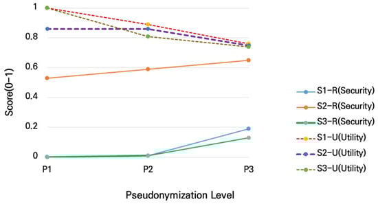
Figure 1.
Changes in security and utility by pseudonymization level (P1–P3) across scenarios. The X-axis represents pseudonymization levels (P1, P2, P3), and the Y-axis indicates the corresponding values (0–1). For each scenario (S1, S2, S3), security is shown with a solid line and utility with a dashed line, allowing for a visual confirmation of the correlation between stronger pseudonymization and the trade-off between security and utility.
As a real-world validation case, we employed the ACS PUMS Person file (psam_p02, State = 02) [38]. Following the procedures in Section 4.2 and Table 7 (real-world instantiation), we computed Safety (R), Utility (U), and Balance (RUT) under the individual-level attribute schema. Given that the distributions of AGEP, SEX, RAC1P, HISP, SCHL, MAR, and PINCP directly affect the EC structure and external matching rates, the qualitative trend matches the synthetic experiments, while absolute values and change magnitudes may differ.
As shown in Table 10, the real-world dataset (psam_p02) exhibited the expected inverse relationship between safety and utility: safety () increased steadily from 0.374 → 0.784 → 0.926, while utility () decreased from 0.997 → 0.858 → 0.758 as pseudonymization strength rose from P1 to P3. The balance index () followed the pattern P1 (0.686) < P2 (0.821) < P3 (0.842), indicating that P2 already achieved a high level of balance, with P3 providing only marginal improvement at the cost of reduced utility. This qualitative trend is consistent with the synthetic-data experiments and aligns with the theoretical expectation that stronger generalization and coarsening lower internal and external risks while reducing analytical utility. Practically, P2 represents a balanced setting when utility is prioritized, whereas P3 is preferable when maximizing safety is critical.
Table 10.
Results of Safety, Utility, and Balance on Real-World Data (ACS PUMS Person: psam_p02, State = 02) [38], computed according to the formulas defined in Table 8.
Figure 2 further illustrates the trajectory of the proposed balance index (RUT). S2 maintained the highest balance values across all pseudonymization levels, while S1 and S3 exhibited greater volatility. These findings indicate that data distribution characteristics—balanced, skewed, or rare—are critical determinants of pseudonymization effectiveness. In practice, this means that the same pseudonymization rules may lead to very different balance outcomes depending on data characteristics, highlighting the importance of prior distributional analysis when designing privacy-preserving data strategies.
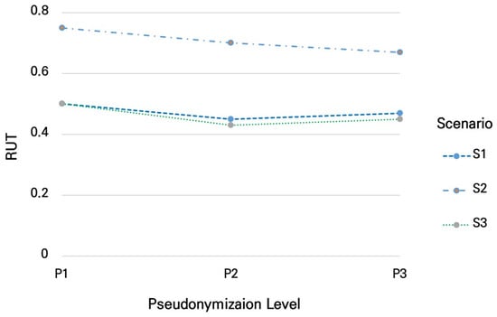
Figure 2.
Trends in the balance metric (RUT) by pseudonymization level across scenarios. The X-axis represents pseudonymization levels (P1, P2, P3), and the Y-axis shows the balance metric RUT (0–1). Different markers and line patterns are used for each scenario to compare how the balance metric changes with increasing levels of pseudonymization.
Before selecting a pseudonymization level, it is desirable to conduct a simple diagnostic procedure to understand the data’s distributional characteristics and identify factors that influence the balance between safety and utility.
This study proposes the following stepwise approach:
- Marginal distributions
For all major attributes used in the analysis, compute histograms—incorporating weights when available—to examine the degree of skewness and tail concentration (e.g., top 1% share).
- Equivalence class sparsity
Calculate the equivalence class size (EC) for combinations of attributes and summarize the distribution using the proportion of records with and the 5th, 50th, and 95th percentiles to capture the prevalence of rare combinations.
- Rare-combination rate
Measure the share of records with small EC values (e.g., ) to anticipate internal re-identification risk.
- Utility sensitivity preview
Simulate the candidate pseudonymization levels (P1–P3) by applying the corresponding range reduction or rounding units and compute distributional similarity (cosine or Jaccard) and normalized loss (e.g., MAD) in a single scan to preview expected utility degradation trends.
This procedure is a lightweight diagnostic analysis: each step can be performed with a single data scan using key-based aggregations or fixed-bin histograms. Therefore, it can efficiently scale in distributed environments such as Spark or MapReduce. If full access to the dataset is limited, the analysis can be approximated using a stratified sample with survey weights or by applying streaming sketch techniques (e.g., t-digest) to estimate frequencies and quantiles. If even these summaries cannot be generated, it is advisable to adopt conservative defaults—such as broader attribute categories or higher pseudonymization levels (P2–P3)—and explicitly report sensitivity bands across plausible distributional scenarios. The resulting EC spectrum and rare-combination rate provide insight into the data’s safety risk level, while the similarity and loss estimates indicate the degree of utility reduction. Taken together, these diagnostics help determine whether an intermediate pseudonymization level (P2) offers a balanced outcome or whether stronger generalization (P3) is required under higher linkage risk.
5. Conclusions and Future Research Directions
This paper introduced RUT, a unified metric that summarizes safety–utility trade-offs under pseudonymization by combining risk- and utility-based components. Using synthetic datasets and a real-world subset of ACS PUMS (State = 02), we observed a consistent qualitative pattern: stronger pseudonymization generally increases safety while decreasing utility, with a mid-range setting often providing a favorable balance. These results indicate that RUT can serve as a useful organizing lens for comparing policy options across levels of generalization and coarsening.
That said, our claims are bounded by the present scope. First, empirical validation spans one synthetic generator and one real-world dataset and therefore does not capture the full diversity of domains or adversary models. Second, while we provided weight-selection guidelines and a sensitivity protocol for , further sector-specific calibration and decision thresholds warrant investigation. Third, we analyzed computational complexity at the algorithmic level and argued practical scalability via aggregation-centric implementations; full at-scale deployments should still be profiled under production constraints (e.g., memory pressure, skewed key spaces).
Accordingly, we view RUT as a promising and extensible evaluation construct rather than a definitive standard. Future work will (i) broaden real-world validation across multiple sectors and jurisdictions, (ii) integrate regulatory or mission-driven constraints more directly into weight selection and reporting, and (iii) release distributed implementations with reproducible benchmarks at larger scales. Within these limits, our results suggest that RUT can support practical decision-making by making the safety–utility balance explicit and comparable, while leaving room for application-specific tailoring.
Funding
This research was partly supported by the Institute of Information & Communications Technology Planning & Evaluation—Information Technology Research Center (IITP-ITRC) grant funded by the Korea government (MSIT) (IITP-2025-RS-2024-00438056). Additionally, this research was supported by the Regional Innovation System & Education (RISE) program through the Gangwon RISE Center, funded by the Ministry of Education (MOE) and the Gangwon State (G.S.), Republic of Korea (2025-RISE-10-008).
Data Availability Statement
The raw data supporting the conclusions of this article will be made available by the authors on request.
Conflicts of Interest
The author declares no conflicts of interest. The funders had no role in the design of the study; in the collection, analyses, or interpretation of data; in the writing of the manuscript; or in the decision to publish the results.
Abbreviations
The following abbreviations are used in this manuscript:
| RUT | Relative Utility–Threat |
References
- Ohm, P. Broken promises of privacy. UCLA Law Rev. 2010, 57, 1701–1777. [Google Scholar]
- Barth-Jones, D.C. The “Re-Identification” of Governor William Weld’s Medical Information: A Critical Re-Examination. 2012. Available online: https://papers.ssrn.com/sol3/papers.cfm?abstract_id=2076397 (accessed on 15 August 2025).
- Rocher, L.; Hendrickx, J.M.; de Montjoye, Y.-A. Estimating the success of re–identifications in incomplete datasets using generative models. Nat. Commun. 2019, 10, 3069. [Google Scholar] [CrossRef] [PubMed]
- Wu, X.; Zhu, X.; Wu, G.Q.; Ding, W. Data mining with big data. IEEE Trans. Knowl. Data Eng. 2014, 26, 97–107. [Google Scholar] [CrossRef]
- Lee, J.; Kim, Y.; Choi, S. Risk–adaptive pseudonymization in big data environments. IEEE Access 2024, 12, 51234–51248. [Google Scholar]
- Aggarwal, C.C. Recent advances in privacy–preserving data publishing: An overview. ACM Comput. Surv. 2022, 54, 1–44. [Google Scholar]
- Fung, B.C.M.; Wang, K.; Chen, R.; Yu, P.S. Privacy–preserving data publishing: A survey of recent developments. ACM Comput. Surv. 2010, 42, 1–53. [Google Scholar] [CrossRef]
- Narayanan, A.; Shmatikov, V. Robust De–anonymization of Large sparse datasets. In Proceedings of the 2008 IEEE Symposium on Security and Privacy (sp 2008), Oakland, CA, USA, 18–21 May 2008; pp. 111–125. [Google Scholar] [CrossRef]
- Rodriguez, A.; Lewis, S.C.; Eldridge, S.; Jackson, T.; Weir, C.J. A survey on UK researchers’ views regarding their experiences with the de–identification, anonymisation, release methods and re–identification risk estimation for clinical trial datasets. Clin. Trials 2025, 22, 11–23. [Google Scholar] [CrossRef]
- Sweeney, L. k–anonymity: A model for protecting privacy. Int. J. Uncertain. Fuzziness Knowl. Based Syst. 2002, 10, 557–570. [Google Scholar] [CrossRef]
- Domingo-Ferrer, J.; Torra, V. A Critique of k-Anonymity and Some of Its Enhancements. In Proceedings of the 2008 Third International Conference on Availability, Reliability and Security, Barcelona, Spain, 4–7 March 2008; pp. 990–993. [Google Scholar] [CrossRef]
- El Emam, K.; Dankar, F.K. Protecting privacy using k–anonymity. J. Am. Med. Inform. Assoc. 2008, 15, 627–637. [Google Scholar] [CrossRef]
- Aggarwal, C.C. On k–anonymity and the curse of dimensionality. In Proceedings of the 31st VLDB Conference, Trondheim, Norway, 30 August–2 September 2005. [Google Scholar]
- Machanavajjhala, A.; Gehrke, J.; Kifer, D.; Venkitasubramaniam, M. L–diversity: Privacy beyond k–anonymity. In Proceedings of the 22nd International Conference on Data Engineering (ICDE’06), Atlanta, GA, USA, 3–7 April 2006; p. 24. [Google Scholar] [CrossRef]
- Li, N.; Li, T.; Venkatasubramanian, S. t-Closeness: Privacy Beyond k-Anonymity and l-Diversity. In Proceedings of the 2007 IEEE 23rd International Conference on Data Engineering, Istanbul, Turkey, 17–20 April 2007; pp. 106–115. [Google Scholar] [CrossRef]
- Gkoulalas-Divanis, A.; Loukides, G. Privacy–enhancing technologies in the era of big data analytics. Wiley Interdiscip. Rev. Data Min. Knowl. Discov. 2020, 10, e1331. [Google Scholar]
- Sarmin, F.J.; Sarkar, A.R.; Wang, Y.; Mohammed, N. Synthetic data: Revisiting the privacy-utility trade-off. Int. J. Inf. Secur. 2025, 24, 156. [Google Scholar] [CrossRef]
- Adams, T.; Birkenbihl, C.; Otte, K.; Ng, H.G.; Rieling, J.A.; Näher, A.F.; Sax, U.; Prasser, F.; Fröhlich, H.; Alzheimer’s Disease Neuroimaging Initiative. On the fidelity versus privacy and utility trade-off of synthetic patient data. iScience 2025, 28, 112382. [Google Scholar] [CrossRef]
- Zhou, Y.; Malin, B.; Kantarcioglu, M. SMOTE–DP: Improving privacy–utility tradeoff with synthetic data. arXiv 2025, arXiv:2506.01907. [Google Scholar]
- Giddens, S.; Liu, F. SAFES: Sequential privacy and fairness enhancing data synthesis. arXiv 2024, arXiv:2411.09178. [Google Scholar] [CrossRef]
- Guillaudeux, M.; Rousseau, O.; Petot, J.; Bennis, Z.; Dein, C.A.; Goronflot, T.; Vince, N.; Limou, S.; Karakachoff, M.; Wargny, M.; et al. Patient-centric synthetic data generation, no reason to risk re-identification in biomedical data analysis. npj Digit. Med. 2023, 6, 37. [Google Scholar] [CrossRef] [PubMed]
- Stadler, T.; Oprisanu, B.; Troncoso, C. Synthetic data—Anonymisation Groundhog Day. In Proceedings of the 31st USENIX Security Symposium, Boston, MA, USA, 10–12 August 2022; pp. 1451–1468. [Google Scholar]
- Jiang, Y.; Mosquera, L.; Jiang, B.; Kong, L.; El Emam, K. Measuring re–identification risk using a synthetic estimator to enable data sharing. PLoS ONE 2022, 17, e0269097. [Google Scholar] [CrossRef]
- Murtaza, H.; Ahmed, M.; Farooq Khan, N.; Murtaza, G.; Zafar, S.; Bano, A. Synthetic data generation: State of the art in health care domain. Comput. Sci. Rev. 2023, 48, 100546. [Google Scholar] [CrossRef]
- Dwork, C.; Roth, A. The algorithmic foundations of differential privacy. FNT Theor. Comput. Sci. 2014, 9, 211–407. [Google Scholar] [CrossRef]
- Abowd, J.M. The U.S. Census Bureau adopts differential privacy. In Proceedings of the 24th ACM SIGKDD, London, UK, 19–23 August 2018; ACM: New York, NY, USA, 2018; p. 2867. [Google Scholar] [CrossRef]
- Cummings, R. Advancing differential privacy: Where we are now and where we should be headed. Harv. Data Sci. Rev. 2024, 6. Available online: https://hdsr.mitpress.mit.edu/pub/sl9we8gh (accessed on 15 August 2025).
- Near, J.P.; Darais, D. Guidelines for Evaluating Differential Privacy Guarantees. NIST SP 800-226. 2023. Available online: https://nvlpubs.nist.gov/nistpubs/SpecialPublications/NIST.SP.800-226.ipd.pdf (accessed on 15 August 2025).
- Park, H.; Lim, D.; Shin, Y. Differential privacy for skewed datasets: Improving utility with adaptive noise. Expert Syst. Appl. 2023, 225, 120123. [Google Scholar]
- Fazênvia, M. Data slots: Trade–offs between privacy concerns and information needs. Humanit. Soc. Sci. Commun. 2025, 12, 643. Available online: https://www.nature.com/articles/s41599-025-04776-1 (accessed on 15 August 2025).
- Xu, W.; Li, C.; Zhang, Y. Utility–preserving privacy–preserving data publishing. Data Sci. J. 2022, 21, 5. [Google Scholar]
- Zhang, T.; Wang, S.; Chen, X. Generative models for privacy–utility trade–off optimization. Inf. Sci. 2023, 627, 555–572. [Google Scholar]
- Mesana, P.; Vial, G.; Jutras, P.; Caporossi, G.; Crowe, J.; Gambs, S. Measuring privacy/utility tradeoffs of format-preserving strategies for data release. J. Bus. Anal. 2025, 8, 147–169. [Google Scholar] [CrossRef]
- Ponte, G.R. Where’s Waldo? A framework for quantifying privacy. Comput. Secur. 2024, 41, 529–546. Available online: https://www.sciencedirect.com/science/article/pii/S0167811624000417 (accessed on 15 August 2025).
- Sondeck, L.P.; Laurent, M. Practical and ready-to-use methodology to assess the re-identification risk in anonymized datasets. Sci. Rep. 2025, 15, 23223. [Google Scholar] [CrossRef]
- Shlomo, N.; Skinner, C.J. Measuring risk of re-identification in microdata: State–of–the–art and new directions. J. R. Stat. Soc. A 2022, 185, 1644–1662. [Google Scholar] [CrossRef]
- Xia, W.; Liu, Y.; Wan, Z.; Vorobeychik, Y.; Kantacioglu, M.; Nyemba, S.; Clayton, E.W.; Malin, B.A. Enabling realistic health data re–identification risk assessment through adversarial modeling. J. Am. Med. Inform. Assoc. 2021, 28, 744–752. [Google Scholar] [CrossRef]
- U.S. Census Bureau. American Community Survey (ACS) 2023 1-Year PUMS File ReadMe. American Community Survey Office, 17 October 2024. Available online: https://www.census.gov/programs-surveys/acs/microdata/documentation.html (accessed on 30 October 2025).
Disclaimer/Publisher’s Note: The statements, opinions and data contained in all publications are solely those of the individual author(s) and contributor(s) and not of MDPI and/or the editor(s). MDPI and/or the editor(s) disclaim responsibility for any injury to people or property resulting from any ideas, methods, instructions or products referred to in the content. |
© 2025 by the author. Licensee MDPI, Basel, Switzerland. This article is an open access article distributed under the terms and conditions of the Creative Commons Attribution (CC BY) license (https://creativecommons.org/licenses/by/4.0/).