Neural Network-Aided Hybrid Particle/FIR Filter for Indoor Localization Using Wireless Sensor Networks

Abstract

Indoor localization based on range measurements in wireless sensor networks involves nonlinear measurement models and is susceptible to non-Gaussian noise, which is associated with complex indoor environments. While particle filters (PFs) are well-suited to such systems, they suffer from sample impoverishment, whereby a diminishing sample diversity leads to failures under various conditions. Hence, this paper proposes a novel hybrid localization algorithm that combines a PF, a finite impulse response (FIR) filter, and an artificial neural network. In the proposed algorithm, the PF serves as the main filter for localization because it performs excellently in nonlinear, non-Gaussian systems under normal operation. The neural network is trained to classify whether the system is operating normally or experiencing a failure, based on estimation results from the PF. If a PF failure is detected by the network, the assisting FIR filter is activated to recover the PF from failures. The localization accuracy and reliability of the proposed neural network-aided hybrid particle/FIR filter are confirmed via comparisons with existing algorithms.

1. Introduction

The advancement of mobile robot technology has been accompanied by a concomitant increase in the use of mobile robots in various applications. The utilization of mobile robots has expanded to include food service in restaurants, package sorting in logistics centers, and assembly processes in automobile factories. As the workspaces for these robots are complex indoor environments, the robots are at risk of colliding with people and other robots. To ensure that robots can successfully navigate to their target locations in such spaces while avoiding collisions, they must be equipped with precise and highly reliable real-time localization technology [1,2,3].

Indoor localization frequently utilizes wireless sensor networks (WSNs) based on ultrawideband (UWB) communication technology [4,5,6]. In UWB-based WSNs, anchors are installed at fixed locations with known coordinates, and tags are attached to robots whose positions need to be tracked. The distance between an anchor and a tag is determined by measuring the propagation time of the UWB signal between them. The distance measured from three or more anchors to the tag can be used to estimate the robot’s 2D position through triangulation. Typically, anchors are placed at elevated positions to prevent obstacles from interfering with signal transmission/reception. In rectangular indoor spaces, four anchors are typically installed at each corner. In indoor environments, the presence of numerous obstacles can impede the efficient transmission and reception of radio waves. This phenomenon, known as non-line-of-sight conditions, can cause multipath effects, which introduce non-Gaussian noise into the measurements [7,8,9,10].

State estimation algorithms are used to estimate the state variables of a system based on noisy sensor measurements, and they have been extensively employed for localization. Regarding indoor localization using WSNs, where the measurement model is nonlinear and non-Gaussian noise frequently occurs, particle filters (PFs) have demonstrated superior localization performance compared with other algorithms [11,12,13,14,15]. However, PFs suffer from a phenomenon known as sample impoverishment, characterized by filter malfunction due to insufficient particle diversity [16,17,18,19]. Extensive research has been conducted to address this issue. Specifically, the hybrid particle/finite impulse response (FIR) filter (HPFF) [20,21,22,23] was proposed to recover a PF from failures using an assisting FIR filter. This algorithm is designed to detect failures in the main PF and reset it using the auxiliary FIR filter. Unlike typical recursive state estimation algorithms, the FIR filter can generate estimates using only recent measurements over a finite interval [24,25,26,27,28,29], without requiring initialization; hence, it is suitable as an auxiliary filter operating only occasionally when needed. As PFs demonstrate exceptional estimation accuracy under conditions with nonlinear and non-Gaussian noise, they are used as main filters, while the relatively less accurate FIR filters serve as auxiliary filters. The HPFF achieves accuracy as well as reliability by combining these two complementary types of filters.

This study aims to improve the HPFF using artificial intelligence. Conventional HPFFs detect PF failures based on the Mahalanobis distance between predicted measurements (calculated from estimated positions) and actual measurements. This method enables easy threshold setting based on a chi-square table. However, it may provide false detections when the covariance values of the measurement noise used in the Mahalanobis distance calculations are incorrect. In fact, non-Gaussian noise that differs from the preidentified measurement noise characteristics frequently occurs during position estimation in complex indoor environments. If the covariance of the measurement noise is underestimated, the HPFF’s PF failure detection becomes overly sensitive. Conversely, if it is overestimated, the failure detection becomes overly insensitive, preventing proper PF resetting and degrading localization performance. Therefore, we trained an artificial neural network to detect PF failures by classifying whether the PF’s state is normal or abnormal, using localization data obtained under various noise conditions. When the network determines a PF failure, the auxiliary FIR filter is activated to obtain the estimate and the estimated error covariance. Using the obtained estimates, the FIR filter generates new particles to reset the PF and recover it from the failure. Simulation results regarding localization showed that the proposed neural network-aided HPFF (NN-HPFF) avoided false detection in situations where the measurement noise information was uncertain. We performed UWB-WSN-based localization simulations under normal operating conditions, as well as in cases where the measurement noise covariance was incorrectly known. The NN-HPFF consistently demonstrated superior localization performance without falsely detecting PF failure, even when the measurement noise covariance was misidentified.

The remainder of this paper is organized as follows: Section 2 describes the state-space model required to process WSN measurements as a state estimator in indoor localization. Section 3 describes the proposed NN-HPFF algorithm for indoor localization. Section 4 compares the performance of the NN-HPFF algorithm with that of existing algorithms—PF and HPFF—based on the results of localization simulations. Finally, Section 5 presents the conclusions and discusses future research directions.

2. Related Works

The PF was first proposed by Gordon et al. [30] and has since been widely applied to target-tracking problems with strong nonlinearities [16]. KFs (KFs) and their nonlinear extensions, such as the extended KF [31], unscented KF [32], and cubature KF [33], are all based on the assumption of Gaussian noise; therefore, their estimation accuracy may deteriorate in systems with non-Gaussian noise. In contrast, the PF represents the distribution of state variables using a set of random particles and corresponding weights, achieving excellent performance in nonlinear and non-Gaussian systems. However, PFs suffer from a chronic issue known as sample impoverishment (particle degeneracy or collapse) [17], which occurs when the diversity of particles is lost and only similar or identical particles remain, making accurate state estimation impossible. To address this problem, algorithms such as the regularized PF and unscented PF have been developed, along with many other variants [18,19,34,35,36] that continue to appear. The history of PF research can be viewed as a continuous effort to overcome the problem of sample impoverishment. Most of these algorithms improve the sampling or resampling process to prevent the occurrence of particle depletion.

Robot localization using PFs was first introduced by Thrun et al. under the name Monte Carlo Localization (MCL) [37]. MCL also suffered from sample impoverishment, which led to the development of the mixture MCL algorithm [38], in which the order of sampling and resampling is modified to mitigate this issue. That study reported that the PF failed under conditions such as the kidnapped robot problem, where a robot is suddenly moved to a distant location by an external agent, or when sensors are overly accurate and the measurement noise covariance is extremely small, both of which cause sample impoverishment and consequent PF failure.

Although it shares the same name as the FIR filter used in signal processing, the FIR filter for state estimation is a completely different algorithm. It was originally developed to address the well-known problem of filter divergence in the KF and can be traced back to Jazwinski’s limited-memory filter [39]. Filter divergence in the KF arises from a variety of sources, including modeling errors, numerical errors (such as rounding or quantization), and measurement errors. These errors accumulate over time within the infinite-memory (or infinite impulse response) structure of the KF, where each new estimate continuously incorporates all past information through repeated prediction and correction. To resolve this problem, the FIR filter [24,25,26,27,29,40,41] was developed to use only a limited set of recent data. Algorithms based on this concept are known by various names, such as finite memory estimation [42,43,44] or moving horizon estimation [45]. Because the FIR filter uses only recent information, it responds sensitively to system changes and prevents errors from propagating or accumulating. Consequently, the FIR filter provides highly robust estimation performance in the presence of modeling, computational, or measurement errors that degrade the performance of the KF.

The HPFF is not an algorithm designed to improve the sampling or resampling processes of the PF in order to prevent failures; rather, it is a framework that resets and recovers the PF when a failure occurs by employing an auxiliary filter. Therefore, HPFF is fundamentally different from the many improved versions of PFs. If the continuously evolving PFs can be compared to modern internal combustion engine vehicles, then HPFF corresponds to a hybrid vehicle that combines an electric motor with an internal combustion engine. HPFF should be regarded not as a single filter but as a framework combining a PF and an FIR filter. Whereas conventional PFs focus on preventing failure, HPFF provides a recovery mechanism that resets and restarts the PF when it fails, even after applying improved variants. The key idea of HPFF is to use a PF as the main filter, which is robust in nonlinear and non-Gaussian environments, and an FIR filter as the auxiliary filter, which is less accurate but highly robust and operates in a batch-processing manner over a limited recent time window without updating its initial state. This approach maximizes the advantages of both filters. The FIR filter operates only when PF failure is detected, not in parallel with the PF, resulting in a minimal computational burden. HPFF was originally developed by the present author [20] and has since been applied to various problems [21,22]. Most existing studies combining PFs and FIR filters are based on this work or have directly adopted the HPFF framework for different applications [23].

The second core aspect of HPFF lies in detecting the failure of the PF. When HPFF was first developed, neural network and deep learning technologies were not yet advanced, so the algorithm employed the Mahalanobis distance to detect PF failure. Recently, with the rapid development of neural networks, which have demonstrated outstanding performance in classification and fault detection, the Mahalanobis distance-based method has been replaced by neural network-based detection. Although many studies have combined PFs with neural networks for system fault detection, to the authors’ knowledge, no research has focused on detecting PF failures themselves using neural networks. The NN-HPFF proposed in this study employs a neural network to detect PF failure, providing higher reliability than the conventional Mahalanobis distance-based approach. Experimental results demonstrate that even when the conventional HPFF falsely detects a PF failure, the NN-HPFF correctly identifies it, showing that NN-HPFF reduces false detections and consequently improves reliability and estimation accuracy compared with the traditional HPFF.

Because NN-HPFF is a modular framework, its components—the PF, FIR filter, and neural network—can be replaced with other versions. Using more advanced modules may further enhance performance. However, this study does not aim to investigate how much the estimation accuracy can be improved by specific module combinations. Instead, its objective is to demonstrate that replacing the conventional Mahalanobis distance-based failure detection in HPFF with a neural network can effectively reduce false detections and improve the reliability of the hybrid framework.

3. State-Space Models for WSN-Based Indoor Localization

This section describes a state-space model for indoor localization based on a UWB-WSN. State estimation algorithms such as PFs estimate state variable values using a state-space model and sensor measurements. The state-space model consists of two equations, namely the state equation and the measurement equation, also referred to as the motion model and measurement model, respectively, in position estimation (localization) problems.

3.1. Motion Model

A motion model is an equation describing the motion of the target whose position is to be tracked, i.e., how the target’s position and velocity change over time. The choice of motion model depends on whether information about how the motion state will change in the future is available. When a robot or autonomous vehicle estimates its own position, it has access to the control command information that alters its motion state; hence, it uses a motion model incorporating control inputs. However, when the subject and object of localization differ and information about motion changes is unavailable, a motion model without control inputs must be used. For indoor localization, the estimation subjects vary—people, robots, equipment; moreover, information about motion changes is often unavailable. Therefore, we employ a linear motion model without control inputs: the constant-velocity (CV) motion model.

The CV model is widely used in the field of target tracking. It assumes that the target moves with a constant speed, utilizing equations where velocity changes cannot be known and are thus represented by Gaussian random noise. For 2D localization, we define the state vector at a discrete time k as ${\mathbf{x}}_k={\left[x_k{y}_k{\dot{x}}_k{\dot{y}}_k\right]}^T$, where $(x_k,y_k)$ and $({\dot{x}}_k,{\dot{y}}_k)$ represent the target’s 2D position and velocity, respectively. The equation describing the transition of this state vector, i.e., the CV model, is

$$\begin{array}{cc}\hfill {\mathbf{x}}_k& =\mathbf{F}{\mathbf{x}}_{k-1}+\mathbf{G}{\mathbf{w}}_{k-1}\hfill \\ \hfill & =\left[\begin{array}{cccc}1& 0& T& 0\\ 0& 1& 0& T\\ 0& 0& 1& 0\\ 0& 0& 0& 1\end{array}\right]{\mathbf{x}}_{k-1}+\left[\begin{array}{cc}{T}^2/2& 0\\ 0& T^2/2\\ T& 0\\ 0& T\end{array}\right]{\mathbf{w}}_{k-1},\hfill \end{array}$$

(1)

where T is the sampling interval, and ${\mathbf{w}}_{k-1}\in {\mathbb{R}}^2$ is the Gaussian random noise vector, which has a covariance ${\mathbf{Q}}_{k-1}$.

In the CV model, the covariance ${\mathbf{Q}}_{k-1}$ of the process noise ${\mathbf{w}}_{k-1}$ is a critical design parameter. Since ${\mathbf{w}}_{k-1}$ is a variable reflecting the target’s velocity change, an appropriate ${\mathbf{Q}}_{k-1}$ value must be selected to match the magnitude of the target’s velocity change (i.e., acceleration). If the selected ${\mathbf{Q}}_{k-1}$ value is excessively small or large compared with the actual target acceleration, localization accuracy will deteriorate, and in severe cases, the state estimator may diverge.

3.2. Measurement Model

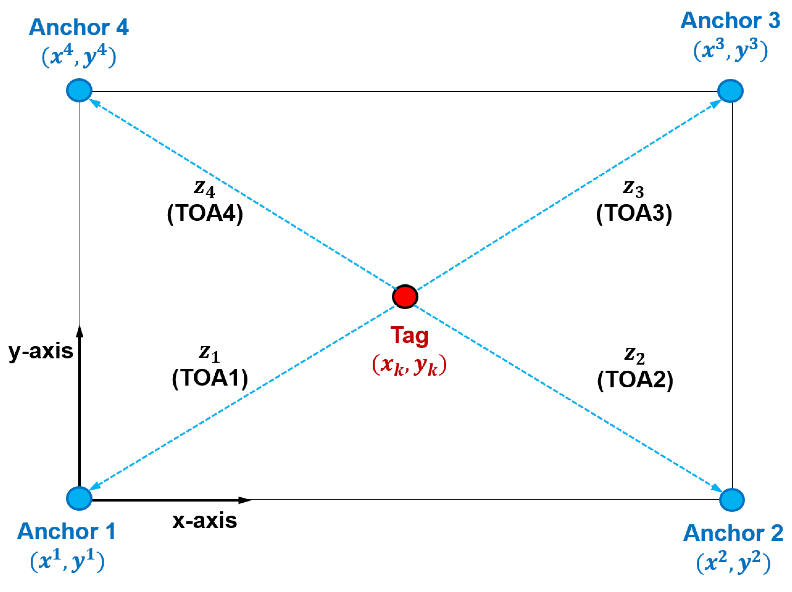
UWB-WSN systems are composed of devices that transmit and receive UWB signals. Anchors are installed at fixed locations within indoor spaces, and their coordinates are provided to the localization system. Tags, which are mobile devices, are attached to objects whose locations are to be tracked. UWB signals are transmitted and received between the anchors and tags, and the tag’s position is calculated using the measurements obtained during this process. The parameters measured in WSNs include the time of arrival, time difference of arrival, angle of arrival, and received signal strength. In this study, we consider the most commonly used parameter, i.e., TOA. As shown in Figure 1, four anchors are placed at the corners of a rectangular indoor space, and their 2D coordinates are assumed to be known. The TOA measurements obtained from these four anchors at a discrete timestep k are expressed as

$$\begin{array}{cc}\hfill z_k^i& ={\displaystyle \frac{1}{c}}\sqrt{{(x_k-x^i)}^2+{(y_k-y^i)}^2},i\in \{1,2,3,4\}\hfill \\ \hfill & =h^i(x_k,y_k),\hfill \end{array}$$

(2)

where $(x^i,y^i)$ represents the fixed 2D coordinates of the i-th anchor, and $h_k^i$ is the nonlinear function used to compute the distance between the target and the i-th anchor.

We define the measurement vector ${\mathbf{z}}_k={\left[z_k^1{z}_k^2{z}_k^3{z}_k^4\right]}^T$ and the measurement function vector as $\mathbf{h}(·)={\left[h^1(·)h^2(·)h^3(·)h^4(·)\right]}^T$. Then, the measurement equation can be written as

$$\begin{array}{cc}\hfill {\mathbf{z}}_k& =\mathbf{h}\left({\mathbf{x}}_k\right)+{\mathbf{v}}_k,\hfill \end{array}$$

(3)

where ${\mathbf{v}}_k\in {\mathbb{R}}^4$ is the measurement noise vector. The covariance of this vector is ${\mathbf{R}}_k$, which reflects the measurement accuracy of the sensor; a smaller ${\mathbf{R}}_k$ value indicates higher accuracy. ${\mathbf{R}}_k$ can be obtained from the sensor manual provided by the manufacturer or directly determined through experimentation. However, the TOA measurement noise in WSNs is not always constant; it can vary depending on the distance between the transmitters and the receivers, the influence of obstacles within the space, and changes in the propagation environment. Differences between the actual noise characteristics and the pre-set ${\mathbf{R}}_k$ can degrade not only the system’s localization accuracy but also the accuracy with which divergences in the PF are detected by the HPFF algorithm.

4. NN-HPFF Algorithm for Indoor Localization Using WSN

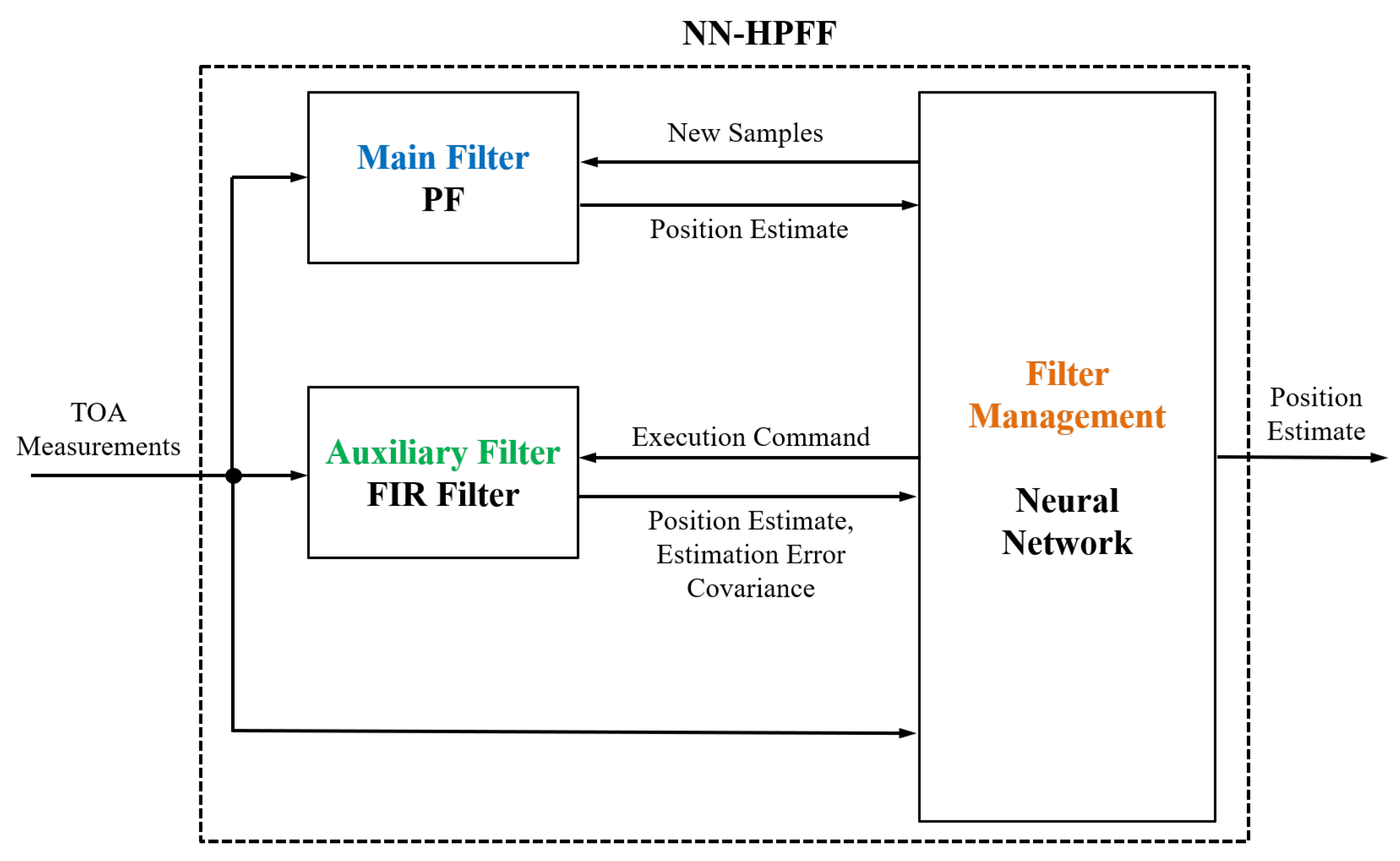
This section outlines the NN-HPFF algorithm for WSN-based localization. The NN-HPFF structure consists of a main filter, an auxiliary filter, and a filter management algorithm based on a neural network for the main filter, as shown in Figure 2.

A PF is employed as the main filter as PFs demonstrate better estimation accuracy than other filters in nonlinear systems with non-Gaussian noise under normal operation. The main filter need not be limited to a specific PF; various state-of-the-art PFs can be used. When a divergence in the main filter is detected, the auxiliary filter is activated to obtain the position estimate and the estimation error covariance. This information is then used to reset the main filter. An FIR filter is used as the auxiliary filter because it employs a batch-processing method. This allows the estimate to be obtained only when needed, without any initial estimate. Recursive filters, such as the KF, require initial values and continuous updates, which renders them unsuitable for operation only during main-filter resets. In contrast, the FIR filter uses only recent information from a finite interval, preventing the accumulation of modeling or computational errors and attaining robustness against divergence. However, since FIR filters use a limited set of measurements for estimation, their estimation accuracy is lower than that of recursive filters under normal conditions. Therefore, using them as auxiliary filters is more appropriate than using them as main filters. As various types of FIR filters exist, selecting an appropriate, up-to-date option is sufficient. The core module of the NN-HPFF, namely the filter management algorithm, trains an artificial neural network to detect failures in the main filter. Upon failure detection, this algorithm issues a command to activate the auxiliary FIR filter, receives the estimated output from the FIR filter, and generates new samples for the PF.

4.1. Localization Using PF

PFs represent the distribution of state variables as a set of random samples and their corresponding weights: ${\{{\mathbf{x}}_k^j,w_k^j\}}_{j=1}^N$, where N is the number of particles. Since the initial position of the target is unknown in indoor localization, the initial samples are generated to be uniformly distributed throughout the indoor space, and all samples are assigned identical weights:

$$\begin{array}{cc}\hfill {\mathbf{x}}_k^j& ={\left[x_k^j{y}_k^j{\dot{x}}_k^j{\dot{y}}^j\right]}^T,\hfill \end{array}$$

(4)

$$\begin{array}{cc}\hfill x_k^j& \sim \mathcal{U}[0,d_x],y_k^j\sim \mathcal{U}[0,d_y],\hfill \end{array}$$

(5)

$$\begin{array}{cc}\hfill {\dot{x}}_k^j& \sim \mathcal{U}[0,v_x],{\dot{y}}_k^j\sim \mathcal{U}[0,v_y],\hfill \end{array}$$

(6)

$$\begin{array}{cc}\hfill w_k^j& ={\displaystyle \frac{1}{N}},\hfill \end{array}$$

(7)

where $\mathcal{U}[a,b]$ represents a uniform distribution over the interval $[a,b]$; $d_x$ and $d_y$ are the width and height of the indoor space, respectively; and $v_x$ and $v_y$ are the maximum velocities of the target along the x and y axes, respectively.

After the initial samples are generated, the PF performs recursive estimation through sampling and resampling steps. The sampling step involves passing the samples through the motion model to obtain temporally updated samples as follows:

$$\begin{array}{cc}\hfill {\mathbf{x}}_k^j& =\mathbf{F}{\mathbf{x}}_{k-1}^j+\mathbf{G}{\mathbf{w}}_{k-1}^j,\hfill \end{array}$$

(8)

$$\begin{array}{cc}\hfill {\mathbf{w}}_{k-1}^j& \sim \mathcal{N}(0,{\mathbf{Q}}_{k-1}),\hfill \end{array}$$

(9)

where $\mathcal{N}(0,{\mathbf{Q}}_{k-1})$ represents a Gaussian distribution with zero mean and a covariance ${\mathbf{Q}}_{k-1}$.

In the resampling step, samples are reselected with probabilities proportional to their weights. The resampling procedure is detailed in [16,17]. Each particle’s weight is assigned such that it is proportional to the following likelihood:

$$\begin{array}{cc}\hfill w_{k-1}^j& ={\displaystyle \frac{{\overline{w}}_{k-1}^j}{{\sum }_{j=1}^N{\overline{w}}_{k-1}^j}},\hfill \end{array}$$

(10)

$$\begin{array}{cc}\hfill {\overline{w}}_{k-1}^j& \sim p\left({\mathbf{z}}_k\right|{\mathbf{x}}_k^j),\hfill \end{array}$$

(11)

where $w_{k-1}^j$ is the normalized weight. Since we assumed the measurement noise to be Gaussian, the likelihood $p\left({\mathbf{z}}_k\right|{\mathbf{x}}_k^j)$ can be computed as

$$\begin{array}{cc}\hfill p\left({\mathbf{z}}_k\right|{\mathbf{x}}_k^j)& ={\displaystyle \frac{1}{{\left(2\pi \right)}^2{\left|{\mathbf{R}}_{\mathbf{k}}\right|}^{1/2}}}\exp \left({\displaystyle \frac{-{({\mathbf{z}}_k-{\widehat{\mathbf{z}}}_k^j)}^T{\mathbf{R}}_k^{-1}({\mathbf{z}}_k-{\widehat{\mathbf{z}}}_k^j)}{2}}\right),\hfill \end{array}$$

(12)

$$\begin{array}{cc}\hfill {\widehat{\mathbf{z}}}_k^j& =\mathbf{h}\left({\mathbf{x}}_k^j\right),\hfill \end{array}$$

(13)

where m denotes the dimension of the measurement vector, and $|{\mathbf{R}}_{\mathbf{k}}|$ represents the matrix determinant of ${\mathbf{R}}_{\mathbf{k}}$.

4.2. Localization Using FIR Filter

FIR filters operate using a batch-processing method. They collect recent measurements over a finite interval, establish an extended matrix from these measurements, and then multiply this matrix by the filter gain to obtain the estimate. This filtering structure obviates the requirement for setting an initial estimate or knowing the covariance of the estimation errors. Moreover, FIR filters do not accumulate modeling errors or computational errors. The measurement interval used in an FIR filter is $[k-M,k-1]$, where M denotes the memory size of the filter. Measurements from the interval $[k-M,k-1]$ are collected to produce an extended matrix ${\mathbf{Z}}_k\in {\mathbb{R}}^{M\times 4}$:

$$\begin{array}{cc}\hfill {\mathbf{Z}}_k& ={[{\mathbf{z}}_m^T{\mathbf{z}}_{m+1}^T\dots {\mathbf{z}}_n^T]}^T,\hfill \end{array}$$

(14)

where $m=k-M$ and $n=k-1$ are the initial and final time points of the FIR filter’s memory, respectively.

The FIR filter produces the state estimate by multiplying ${\mathbf{Z}}_k$ by the filter gain ${\mathbf{L}}_k$:

$$\begin{array}{cc}\hfill {\widehat{\mathbf{x}}}_k& ={\mathbf{L}}_k{\mathbf{Z}}_k.\hfill \end{array}$$

(15)

The gain of an FIR filter is typically determined by solving an optimization problem. We use a minimum-variance FIR (MVF) filter, which minimizes the variance of the estimation error. The MVF filter easily yields the estimation error covariance, which is crucial for generating samples to reset the PF. However, since the MVF filter is a linear filter, it cannot be directly utilized in localization problems with nonlinear measurement equations. Therefore, similar to the process for extended KFs, we first linearize the nonlinear model by computing the Jacobian matrix and then apply the MVF to the linearized model. This yields an extended MVF (EMVF) filter. The gain ${\mathbf{L}}_k$ of the EMVF filter is determined as follows:

$$\begin{array}{cc}\hfill {\mathbf{L}}_k& ={\mathbf{J}}_k{\left[\begin{array}{cc}{\mathbf{W}}_{1,1}& {\mathbf{W}}_{1,2}\\ {\mathbf{W}}_{1,2}^T& {\mathbf{W}}_{2,2}\end{array}\right]}^{-1}\left[\begin{array}{c}{\overline{\mathbf{H}}}_k^T\\ {\overline{\mathbf{G}}}_k^T\end{array}\right]{\overline{\mathbf{R}}}_M^{-1},\hfill \end{array}$$

(16)

$$\begin{array}{cc}\hfill {\mathbf{J}}_k& =[{\mathcal{F}}_{n,m}{\mathcal{F}}_{n,m+1}{\mathcal{F}}_{n,m+2}\dots {\mathcal{F}}_{n,n}I],\hfill \end{array}$$

(17)

$$\begin{array}{cc}\hfill {\mathcal{F}}_{g,h}& =F_g\times F_{g-1}\times F_{g-2}\times \dots \times F_h(g\ge h),\hfill \end{array}$$

(18)

$$\begin{array}{cc}\hfill {\mathcal{F}}_{g,g}& =F_g,\hfill \end{array}$$

(19)

$$\begin{array}{cc}\hfill {\mathbf{W}}_{1,1}& ={\overline{\mathbf{H}}}_M^T{\mathbf{R}}_M^{-1}{\overline{\mathbf{H}}}_M,\hfill \end{array}$$

(20)

$$\begin{array}{cc}\hfill {\mathbf{W}}_{1,2}& ={\overline{\mathbf{H}}}_M^T{\mathbf{R}}_M^{-1}{\overline{\mathbf{G}}}_M,\hfill \end{array}$$

(21)

$$\begin{array}{cc}\hfill {\mathbf{W}}_{2,2}& ={\overline{\mathbf{G}}}_M^T{\mathbf{R}}_M^{-1}{\overline{\mathbf{G}}}_M+{\mathbf{Q}}_M^{-1},\hfill \end{array}$$

(22)

$$\begin{array}{cc}\hfill {\overline{\mathbf{H}}}_N& =\left[\begin{array}{c}{H}_m\\ H_{m+1}{\mathcal{F}}_{m,m}\\ H_{m+2}{\mathcal{F}}_{m+1,m}\\ ⋮\\ H_n{\mathcal{F}}_{n-1,m}\end{array}\right],\hfill \end{array}$$

(23)

$$\begin{array}{cc}\hfill {\overline{\mathbf{G}}}_N& =\left[\begin{array}{ccccc}\mathbf{0}& \mathbf{0}& \dots & \mathbf{0}& \mathbf{0}\\ H_{m+1}& \mathbf{0}& \dots & \mathbf{0}& \mathbf{0}\\ {\mathcal{H}}_{m+2,m+1}& H_{m+2}& \dots & \mathbf{0}& \mathbf{0}\\ ⋮& ⋮& ⋮& ⋮& ⋮\\ {\mathcal{H}}_{n,m+1}& {\mathcal{H}}_{n,m+2}& \dots & H_n& \mathbf{0}\end{array}\right],\hfill \end{array}$$

(24)

$$\begin{array}{cc}\hfill {\mathcal{H}}_{g,h}& =H_g{\mathcal{F}}_{g-1,h}(g>h),\hfill \end{array}$$

(25)

$$\begin{array}{cc}\hfill H_k& ={\left.{\displaystyle \frac{\partial {\mathbf{h}}_k}{\partial \mathbf{x}}}\right|}_{{\widehat{\mathbf{x}}}_k},\hfill \end{array}$$

(26)

$$\begin{array}{cc}\hfill {\overline{\mathbf{R}}}_M& =\left[\mathrm{diag}(\stackrel{M}{\overbrace{{\mathbf{R}}_m{\mathbf{R}}_{m+1}\dots {\mathbf{R}}_n}})\right],\hfill \end{array}$$

(27)

$$\begin{array}{cc}\hfill {\overline{\mathbf{Q}}}_M& =\left[\mathrm{diag}(\stackrel{M}{\overbrace{{\mathbf{Q}}_m{\mathbf{Q}}_{m+1}\dots {\mathbf{Q}}_n}})\right].\hfill \end{array}$$

(28)

The estimation error covariance of the EMVF filter, ${\mathbf{P}}_k$, can be calculated as

$$\begin{array}{cc}\hfill {\mathbf{P}}_k& ={\mathbf{K}}_M{\mathbf{Q}}_M{\mathbf{K}}_M^T+{\mathbf{L}}_k{\mathbf{R}}_M{\mathbf{L}}_k^T,\hfill \end{array}$$

(29)

$$\begin{array}{cc}\hfill {\mathbf{K}}_M& =[{\mathbf{F}}^{M-1}\mathbf{G}{\mathbf{F}}^{M-2}\mathbf{G}\dots \mathbf{FG}\mathbf{G}]\hfill \end{array}$$

(30)

Remark 1.

FIR filters, including the EMVF filter, estimate the state variables using information from a limited time window, and the estimated values are not used to generate the estimates at the next timestep. In other words, at each timestep, the state estimation is performed in a batch-processing manner using only the information within a restricted interval. For this reason, FIR filters possess bounded-input bounded-output (BIBO) stability. The length of the information window used by an FIR filter is called the memory size (M). As M increases, the filter utilizes more information, which improves its noise suppression capability but makes it less sensitive to rapid state changes and reduces robustness to modeling errors. Moreover, a larger M leads to higher computational cost. Conversely, when M decreases, the opposite effects occur. In both HPFF and NN-HPFF, the FIR filter is activated when a PF failure occurs, in order to obtain information needed to recover the PF. PF failures typically occur under conditions of significant modeling errors, parameter uncertainties, or abrupt changes. To achieve robust estimation against such conditions, it is preferable to use a smaller memory size. Therefore, the smallest possible memory size is preferable.

4.3. Filter Management Using Neural Network

The filter management system performs three functions. First, it detects failures in the main filter (PF) using an artificial neural network. Second, upon failure detection, it activates the auxiliary filter (FIR filter) to obtain position estimates and the estimated error covariance. Third, it uses this information to generate new samples for the PF, thereby resetting and rebooting the PF. The core function among these is the detection of PF failures using the neural network. The problem of detecting PF failures does not involve an analysis of time-series data; rather, it is a classification problem that involves analyzing estimation results at a specific time point to determine whether a failure has occurred. Therefore, we selected a feedforward neural network, which is a type of network primarily used for static input processing and classification problems. Information (metrics) that can be used to evaluate the performance of the state estimation algorithm includes the state estimation error, estimation error covariance, and normalized innovation squared (NIS), which is the normalized residual of the measurement. Among these, the state estimation error requires the true values of state variables, which can be obtained only in simulations. Therefore, the state estimation error cannot be used as input for neural networks applied to real systems; it can be used only for training neural networks via simulation. The covariance of the state estimation error is easily obtainable in KFs since they set and update its initial value. However, because PFs use only samples and weights of state variables, they cannot directly calculate this covariance. Instead of the estimated error covariance, the empirical covariance of the particles can be calculated in PFs. However, using this parameter causes numerical instability in situations involving PF failure. This is because during PF failure, the diversity of particles becomes extremely low due to the sample impoverishment phenomenon, which often results in the empirical covariance value being very small, close to zero. Since only a few particles may have significant weights while the majority have very low weights, the calculated empirical covariance may be close to zero. Therefore, empirical covariance is not a suitable indicator for determining PF failure. The NIS is calculated as follows:

$$\begin{array}{cc}\hfill \mathrm{NIS}& ={\mathbf{r}}_k^T{\mathbf{S}}_k^{-1}{\mathbf{r}}_k,\hfill \end{array}$$

(31)

$$\begin{array}{cc}\hfill {\mathbf{r}}_k& ={\mathbf{z}}_k-\mathbf{h}\left({\widehat{\mathbf{x}}}_k\right),\hfill \end{array}$$

(32)

$$\begin{array}{cc}\hfill {\mathbf{S}}_k& ={\mathbf{H}}_k{\mathbf{P}}_k{\mathbf{H}}_k^T+{\mathbf{R}}_k,\hfill \end{array}$$

(33)

where ${\mathbf{r}}_k$ is the residual or innovation. The Jacobian matrix ${\mathbf{H}}_k$ and the estimation error covariance matrix ${\mathbf{P}}_k$ are included in the calculation formula for ${\mathbf{S}}_k$, which either cannot be determined for PFs or causes numerical instability. Therefore, we use ${\mathbf{R}}_k$ instead, which can be viewed as the Mahalanobis distance between the probability distributions of the actual and predicted measurement vectors, and is calculated as follows:

$$\begin{array}{cc}\hfill {\mathcal{D}}_k& ={({\mathbf{z}}_k-{\widehat{\mathbf{z}}}_k)}^T{\mathbf{R}}_k^{-1}({\mathbf{z}}_k-{\widehat{\mathbf{z}}}_k),\hfill \end{array}$$

(34)

$$\begin{array}{cc}\hfill {\widehat{\mathbf{z}}}_k& =\mathbf{h}\left({\widehat{\mathbf{x}}}_k\right),\hfill \end{array}$$

(35)

where ${\widehat{\mathbf{z}}}_k$ is the predicted measurement vector.

${\mathcal{D}}_k$ can be calculated in actual systems instead of only simulations and is therefore used as input to the neural network for detecting PF failures. However, if ${\mathcal{D}}_k$ is the only input, the neural network may lack sufficient feature information for failure detection. Therefore, we also use the absolute output error (AOE) as an input, which is the absolute value of the difference between the prediction for the i-th anchor (the estimated target location and the distance to the i-th anchor) and the actual measurement and is calculated as follows:

$$\begin{array}{cc}\hfill \mathrm{AOE}& = |z_k^i-h_i({\widehat{\mathbf{x}}}_k\left)\right|,i=1,2,3,4.\hfill \end{array}$$

(36)

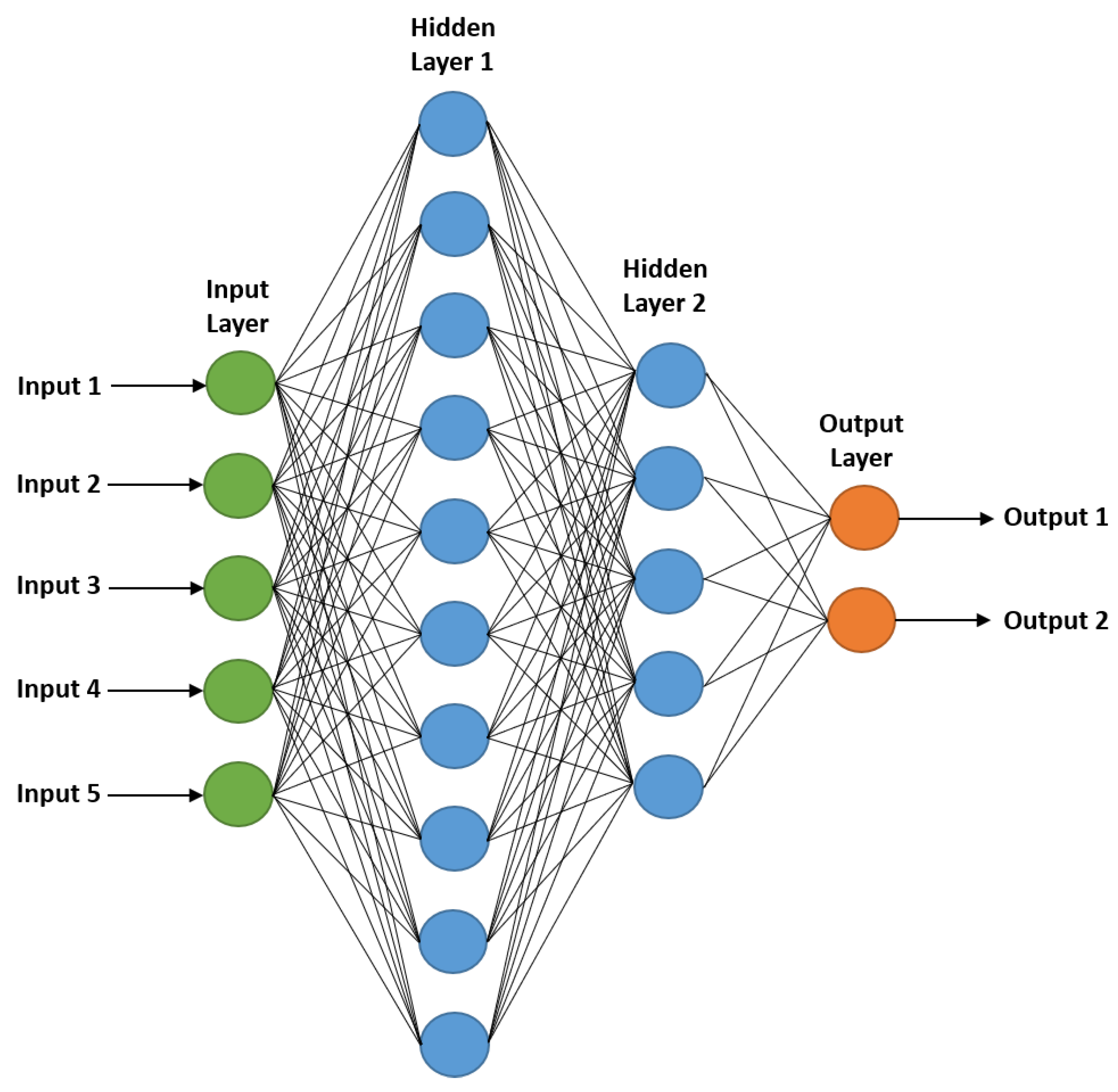
The neural network for PF failure detection uses a total of five inputs: ${\mathcal{D}}_k$ and AOE for the four anchors. The neural network has two output nodes, classifying the PF state into two categories: failure and normal. If the number of hidden layer nodes is too large, computational load increases, slowing processing speed. Therefore, we used 10 nodes in the first hidden layer (twice the number of input nodes) and 5 nodes in the second hidden layer (half the number of the first hidden layer). The neural network structure is shown in Figure 3.

The data used to train the neural network consist of the five input variables described above and their corresponding outputs, which indicate whether or not a PF failure has occurred. This data were generated through localization simulations rather than physical experiments. Conducting experiments under various noise environments and motion conditions of the moving object requires significant time and effort, and it is also difficult to accurately compute the localization error necessary for labeling. The neural network must be trained on data generated under as many diverse conditions as possible to prevent overfitting to specific cases. Therefore, we generated the training data through simulations.

Since the role of HPFF is to detect PF failures, it is necessary to create various conditions under which such failures may occur to obtain training data. The primary parameters that can affect PF failure include the process noise covariance, measurement noise covariance, and the number of particles. Each of these three parameters was assigned three levels: high, medium, and low. Combining these three parameters with three possible levels results in a total of 27 scenarios. Localization simulations of the mobile robot were conducted for all 27 scenarios. In each scenario, the robot traveled for 360 timesteps, performing 360 localization estimates. Each localization result was labeled as either a success or a failure.

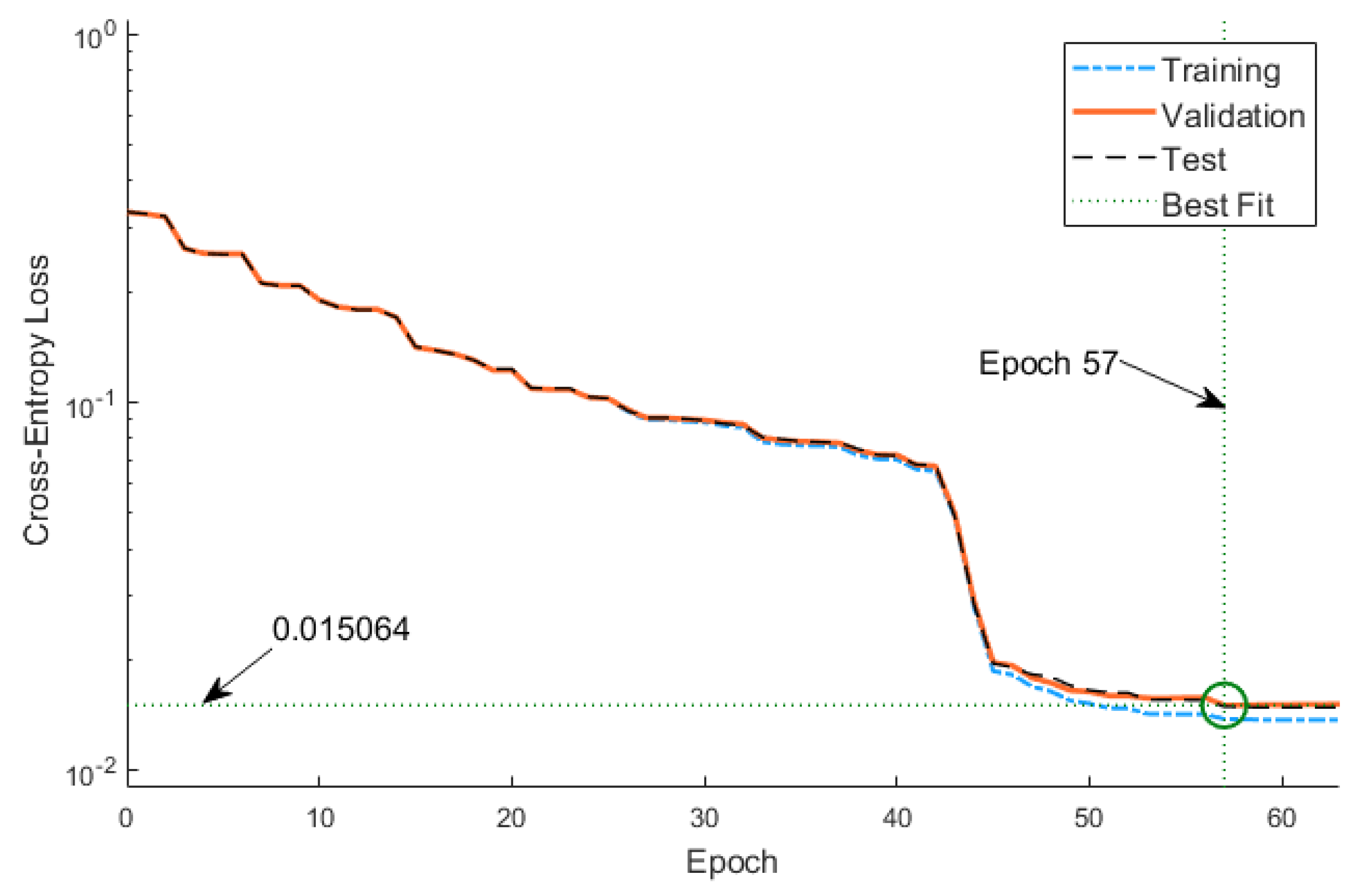
Because the true position of the robot is precisely known in the simulation, the localization error can be calculated accurately. Based on empirical observations, we considered a localization error greater than 0.5 m in UWB-based positioning to indicate failure and used this criterion to identify PF failures. Consequently, 360 data samples were obtained from each of the 27 scenarios, resulting in a total of 9720 samples for neural network training. The neural network was trained using the scaled conjugate gradient method, while the cross-entropy loss function was used as the performance function. The hyperbolic tangent function and the softmax function were used as the activation function for the hidden layer and the output layer, respectively. Figure 4 depicts the learning curve. We terminated the training at Epoch 57. As described above, the neural network is trained offline using the data obtained from 27 scenarios, and the trained network is then used in the NN-HPFF algorithm to detect PF failures.

5. Localization Simulation and Performance Analysis

In this section, the effectiveness of the proposed NN-HPFF is demonstrated through simulations. The conventional HPFF detects PF failure using the Mahalanobis distance, in which the measurement noise covariance is employed. However, in practical applications, the measurement noise covariance is often uncertain and may be selected incorrectly. In the simulations, we consider three cases: when the measurement noise covariance used in the PF is equal to the true covariance of the sensor measurement errors, when it is set larger than the true value, and when it is set smaller. Through these simulations, we show that in the conventional HPFF, an incorrect covariance setting can lead to false detection of PF failure and a consequent degradation in localization accuracy, whereas the proposed NN-HPFF does not suffer from such problems.

To assess the accuracy of a localization algorithm, the error between the estimated and true positions must be calculated. Since the target’s true position is precisely known during simulations, the localization error can be reliably determined, which helps evaluate the algorithm’s performance under various conditions.

The indoor localization scenario was as follows: The indoor space was a square area measuring 10 m × 10 m, with anchors installed at the four corners. One mobile robot equipped with a tag traveled along a square-shaped trajectory. The TOAs between the four anchors and the tag were measured to estimate the mobile robot’s 2D position. The performance of the proposed NN-HPFF algorithm was analyzed by comparing it with the existing HPFF and PF algorithms. The performance metrics were the localization error $e_k$ and the averaged localization error (ALE), calculated as follows:

$$\begin{array}{cc}\hfill e_k& =\sum _{i=1}^{N_{it}}\sqrt{{(x_k-{\widehat{x}}_k)}^2+{(y_k-{\widehat{y}}_k)}^2},\hfill \end{array}$$

(37)

$$\begin{array}{cc}\hfill \mathrm{ALE}& =\sum _{k=1}^{t_f}{e}_k,\hfill \end{array}$$

(38)

where $x_k$ and $y_k$ are the true 2D positions, $t_f$ is the final timestep, and $N_{it}$ represents the number of iterative (Monte Carlo) simulations. In the sampling step of the PF, process noise is randomly generated to produce random particles. Although the process noise covariance remains constant, the random particles generated from it vary at each iteration. Because simulations using random noise yield results that fluctuate from run to run, it is common practice to repeat the same simulation multiple times and compute the statistical average; this procedure is referred to as a Monte Carlo simulation. In this study, simulations were conducted for 27 scenarios, and for each scenario, 100 Monte Carlo simulations were performed. The average of these results was then calculated. Both the localization error and the ALE values represent the averages obtained from the same 100 Monte Carlo simulations.

5.1. Case 1: Ideal Condition

In the first simulation, localization was performed under ideal conditions, where the noise covariance of the sensor measurements was precisely known. The Gaussian noise covariance when generating TOA measurements during the simulation was set to ${\mathbf{R}}_k=0.5^2{\mathbf{I}}_4$, where ${\mathbf{I}}_4$ is the $4\times 4$ identity matrix. Identical measurement noise covariance values were used with both localization algorithms. The process noise covariance in the motion model was set to $Q=0.5^2{\mathbf{I}}_2$, and 5000 particles were used in the PF. The memory size of the EMVF filter, a component of HPFF and NN-HPFF, was set as $M=5$. 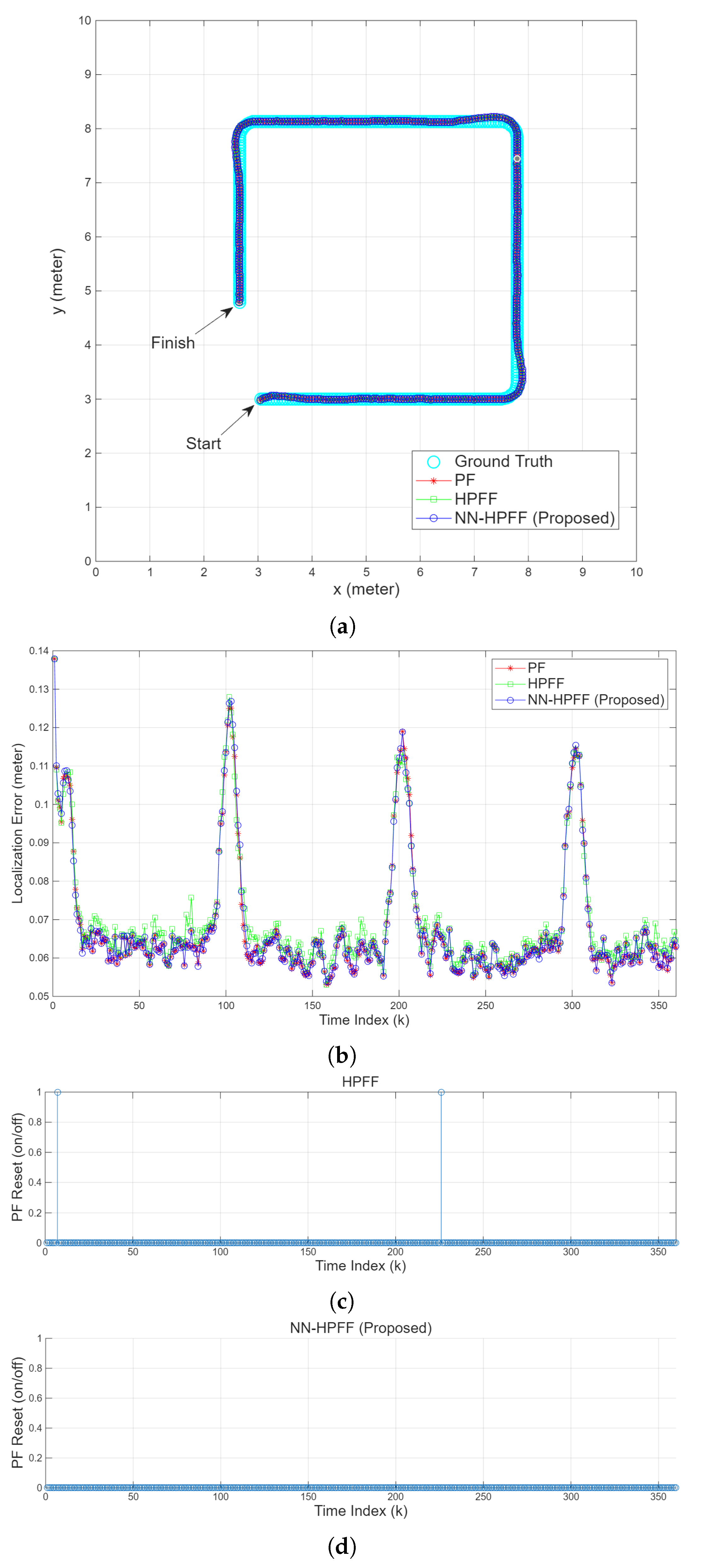Figure 5 presents the results of the localization simulation conducted under these conditions. Figure 5a compares the simulated trajectory of the mobile robot with the trajectories estimated by the algorithms. Since sufficient particles were used and because the values of the process noise and measurement noise covariance were appropriate, the PF operated normally without failure. Thus, the main filter (PF) was rarely reset in either the HPFF or the NN-HPFF. Figure 5c,d show the PF reset timings for HPFF and NN-HPFF, respectively. In these graphs, “1” indicates that a reset was executed, whereas “0” indicates that no reset was executed. Figure 5c shows that a PF reset occurred once with HPFF, but this corresponded to a false detection of PF failure. Figure 5d shows that unlike HPFF, NN-HPFF exhibited no false detections of PF failure and did not execute any PF reset whatsoever. Figure 5b shows the localization errors of the three algorithms as a function of time. The errors exhibited high peaks around timesteps $k=0$, 100, 200, and 300. Near $k=0$, localization had just begun, which resulted in large errors. Because the mobile robot’s initial position was unknown, the initial particles of the PF were randomly generated throughout the indoor space. Consequently, although the localization error was initially large, it gradually decreased as resampling using measurements progressed. Around $k=100$, 200, and 300, the robot approached the corners of the rectangular trajectory. At these points, the robot changed direction; this increased the error of the CV model, consequently increasing the localization error. Under ideal operating conditions, the three algorithms produced nearly identical localization results and were thus difficult to distinguish.

5.2. Case 2: Underestimated Measurement Noise Covariance

The second scenario involved localization when the measurement noise covariance was not precisely known and the noise was underestimated. While the noise covariance of the TOA measurements generated during the simulation was ${\mathbf{R}}_k=0.5^2{\mathbf{I}}_4$, the localization algorithms used a smaller value of $0.1^2{\mathbf{I}}_4$. All other conditions were identical to those in the first scenario. Since PFs function correctly under such conditions, a PF failure was not expected to be detected. The measurement noise covariance is used to calculate the Mahalanobis distance, as shown in Equation (35); accordingly, a PF failure was determined when this value exceeded the threshold. Since the inverse of ${\mathbf{R}}_k$ is used to generate the Mahalanobis distance ${\mathcal{D}}_k$, a smaller ${\mathbf{R}}_k$ increases ${\mathcal{D}}_k$, leading to frequent PF failure detection. 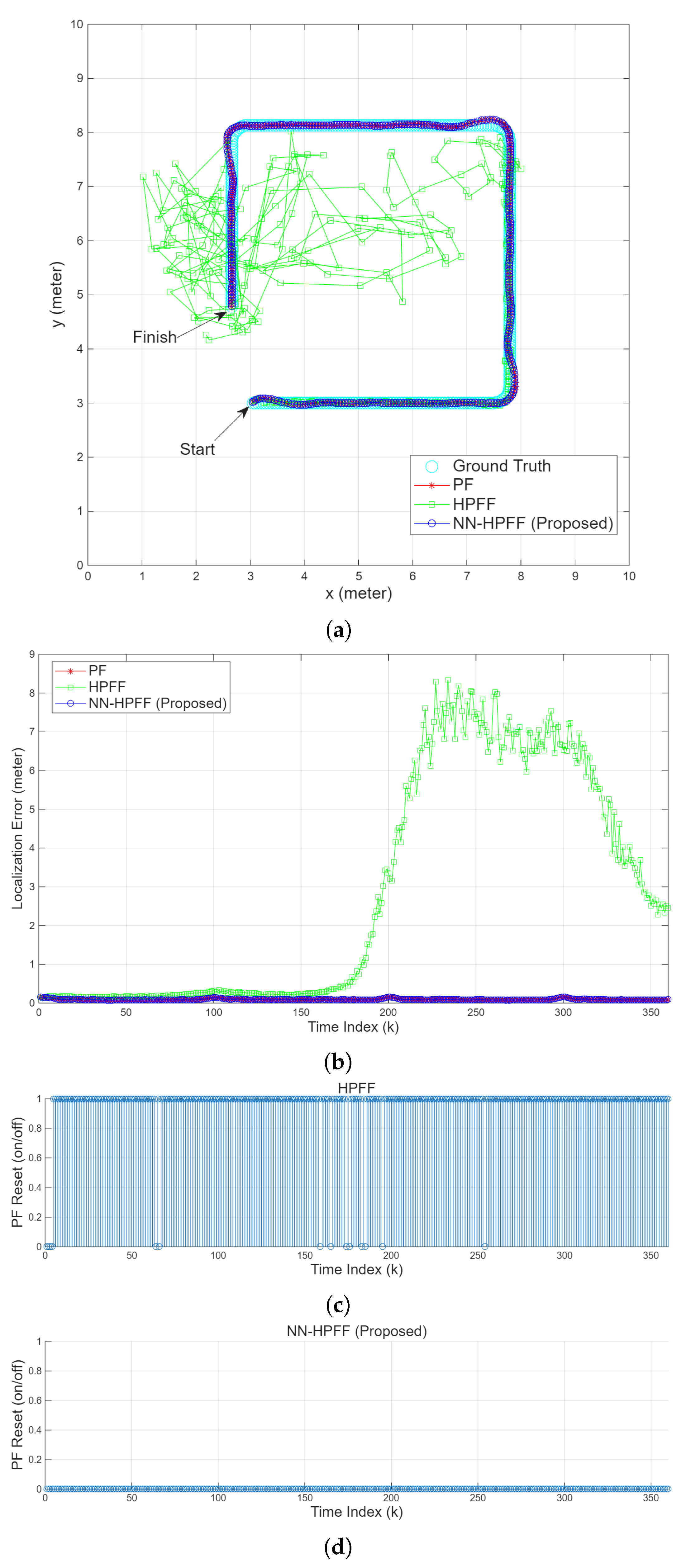Figure 6c shows that PF resets occurred very frequently when using HPFF, which indicates that an underestimated ${\mathbf{R}}_k$ renders HPFF’s PF failure detection overly sensitive. The auxiliary EMVF filter exhibited a lower estimation accuracy than the main PF filter under normal conditions. Excessively triggered PF resets when using the low-accuracy EMVF filter can induce sample impoverishment, significantly increasing the localization error, as seen in Figure 6c. Figure 6d shows that NN-HPFF did not produce any false detections. This is because it utilizes a neural network for failure detection, which uses four AOE values as inputs in addition to the Mahalanobis distance; hence, this algorithm is unaffected by underestimated ${\mathbf{R}}_k$ values. Consequently, NN-HPFF did not perform any PF resets and behaved similarly to a pure PF.

5.3. Case 3: Overestimated Measurement Noise Covariance

The third scenario involved using the localization algorithms with an overestimated measurement noise covariance. The noise covariance used to generate TOA measurements during the simulation was set to ${\mathbf{R}}_k=0.5^2{\mathbf{I}}_4$, while the value used in the localization algorithms was set to ${\mathbf{R}}_k=1^2{\mathbf{I}}_4$. The number of particles was kept at 5000, the same as in the previous two scenarios. 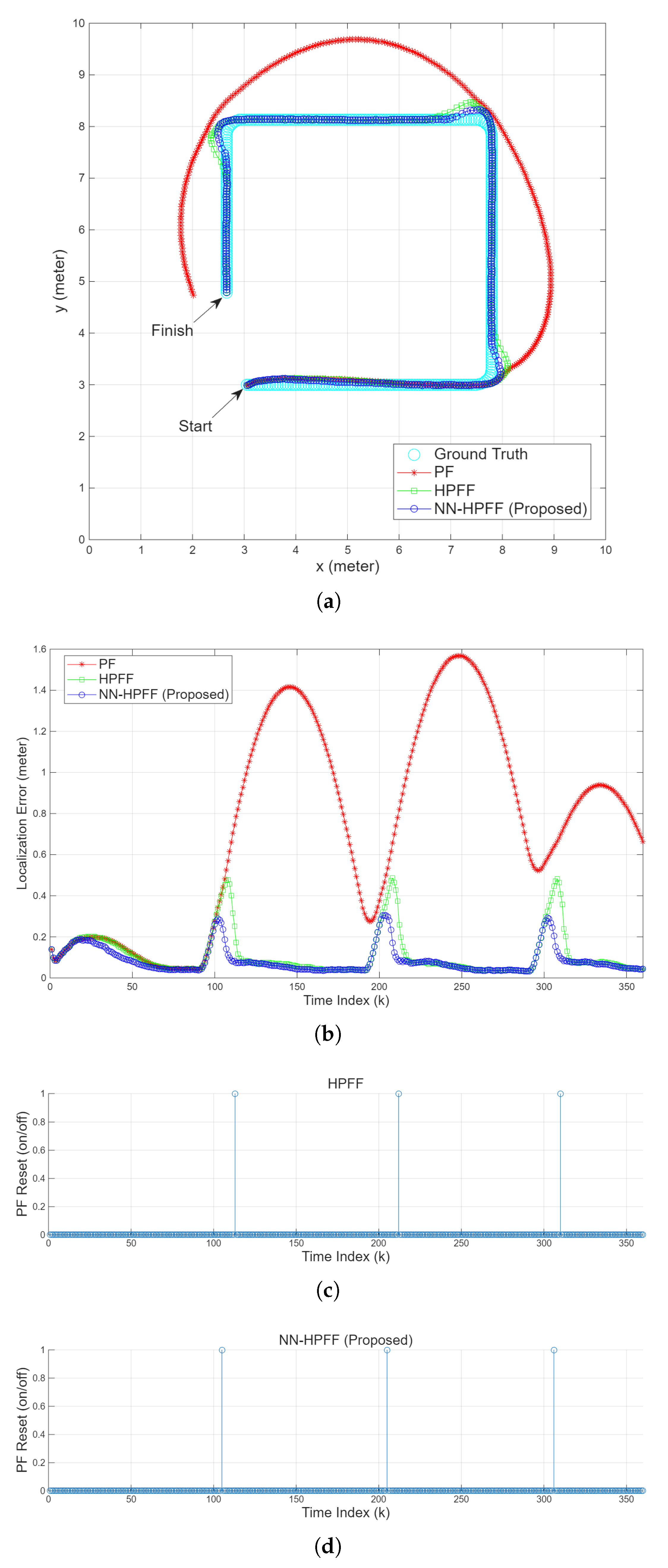However, the process noise covariance was set to a lower value of ${\mathbf{Q}}_k=0.1^2{\mathbf{I}}_2$ to induce sample impoverishment in the PF. Under these conditions, PF failure occurred, specifically when the mobile robot turned the first corner, as shown in Figure 7a. As mentioned earlier, the CV motion model assumes CV motion, which leads to modeling errors when the velocity changes abruptly. While large ${\mathbf{Q}}_k$ values can accommodate velocity changes, a velocity change larger than ${\mathbf{Q}}_k$ reduces the estimation accuracy. When the robot turned a corner, the estimated position initially began to deviate from the actual position, whereafter the deviation gradually diminished. However, when the robot encountered the next corner, the estimated position again started to deviate from the actual position. Figure 7b shows a sharp increase in the PF’s localization error near $k=100$ (the first corner). In such situations, HPFF and NN-HPFF detected the PF’s failure and reset it, causing the error to decrease again and normal operation to resume. However, Figure 7c,d show that HPFF executed the PF reset later than NN-HPFF did. This was because the overestimated ${\mathbf{R}}_k$ caused ${\mathcal{D}}_k$ to decrease, reducing the sensitivity of error detection. Consequently, HPFF exhibited a higher error peak.

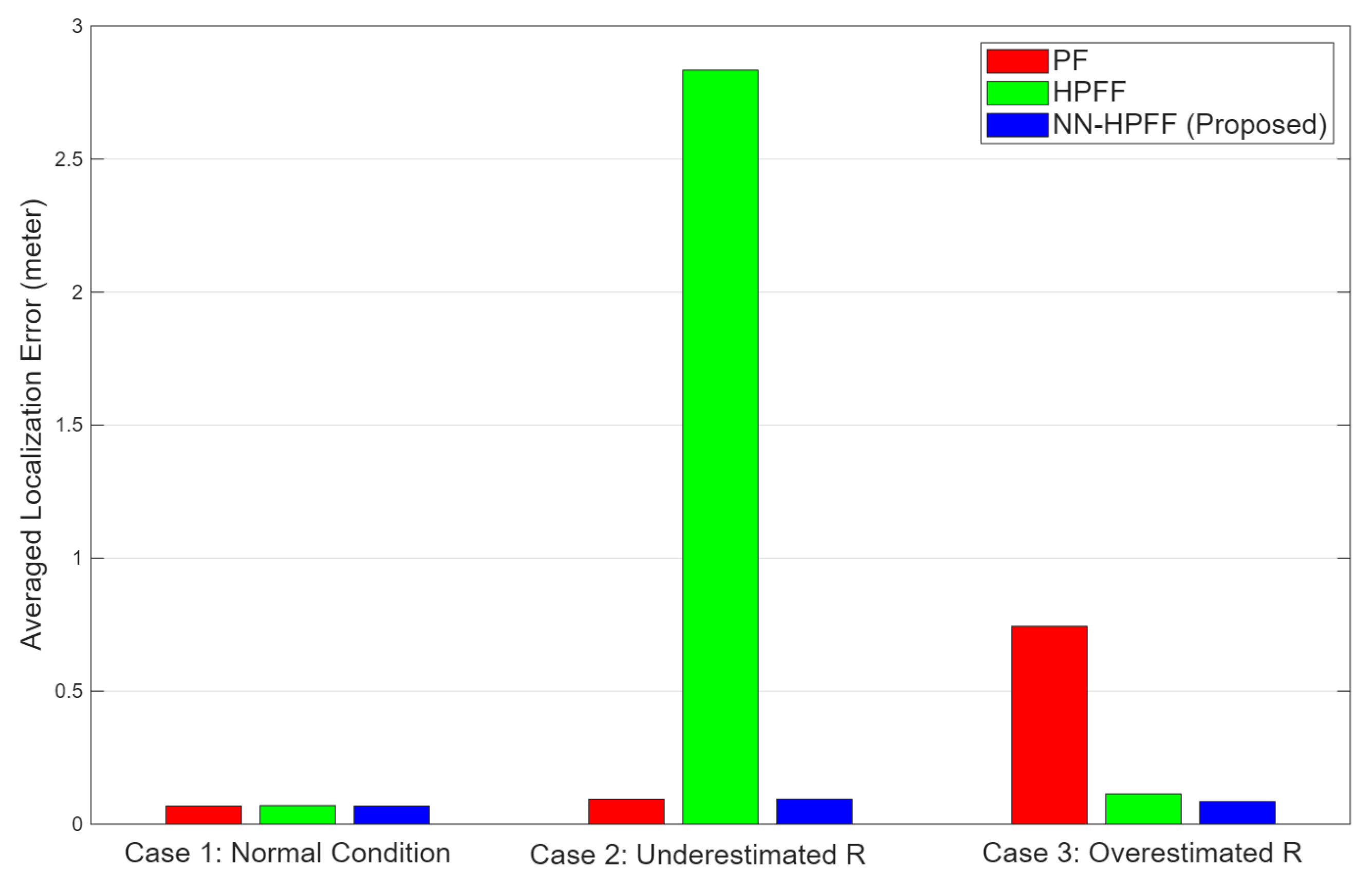
Figure 8 compares the ALE values of the localization algorithms across the three simulation cases. In Case 1, both the process noise and measurement noise are appropriately set, resulting in conditions where PF failures rarely occur. As shown in Figure 8, the PF achieves very low ALE values and highly accurate localization performance. In this case, the measurement noise covariance used in HPFF is identical to the covariance value used to generate the measurement noise in the simulation. Consequently, HPFF produces almost no false detections. Since PF failures hardly occurred in this case, and HPFF accurately detected the absence of failures, both PF and HPFF exhibit nearly identical ALE values. When no PF failure occurs, HPFF does not perform a reset using the FIR filter, yielding results equivalent to the pure PF. Similarly, the NN-HPFF, which detects PF failures using a neural network, also shows nearly the same ALE as the PF, indicating that it did not produce any false detections.

In Case 2, the measurement noise covariance used in HPFF was set lower than the true value. A smaller measurement noise covariance results in an increase in the Mahalanobis distance. Because the covariance was underestimated, the Mahalanobis distance was overestimated, leading to more frequent cases where it exceeded the threshold and incorrectly indicated PF failures. Such false detections caused unnecessary resets using the FIR filter. Since the FIR filter is configured with a minimal memory size to provide a rough estimate for recovery, this unnecessary resetting significantly increased the ALE. When the measurement noise covariance is underestimated, PF failures are falsely detected even when they do not occur, resulting in unnecessary resets and a considerable degradation of localization accuracy. In contrast, NN-HPFF detects PF failures using a neural network classifier, which prevented false detections and thus did not trigger unnecessary FIR filter resets. As a result, NN-HPFF achieved ALE values equivalent to those of the pure PF.

In Case 3, the measurement noise covariance used in HPFF was set higher than the true value. In this case, the Mahalanobis distance was underestimated, making the PF failure detection less sensitive. Consequently, actual PF failures may not be detected. To verify this, the process noise covariance was reduced to intentionally induce PF failures. As shown in Figure 7, PF failures occurred, resulting in increased localization errors. A comparison of Figure 7b–d shows that NN-HPFF detected the increase in PF localization error earlier and performed the reset more promptly, whereas HPFF detected it later, leading to higher peaks in the localization error. However, as shown in Figure 8, the difference in ALE between HPFF and NN-HPFF was not significant. This indicates that setting the measurement noise covariance lower than the actual value, which makes the failure detection overly sensitive, causes more serious problems. From the results of the three simulation cases, it can be concluded that the Mahalanobis distance-based PF failure detection method of HPFF can lead to false detections and degraded localization accuracy when the measurement noise covariance is incorrectly specified. Furthermore, the proposed NN-HPFF successfully resolves the false detection problem caused by uncertainty in the measurement noise covariance.

The number of particles in the PF was set to 5000, and the average time required for each algorithm to perform a single point localization was measured, the results of which are presented in

Table 1. Comparison of average computation time for single point localization.

Algorithm	PF	HPFF	NN-HPFF (Proposed)
Average Computation Time	4.15 ms	4.55 ms	7.01 ms

. The computations were carried out on a computer equipped with an Intel Core i5-12500 (3 GHz) CPU and 16 GB of RAM, without using a GPU. The computation times per iteration for PF and HPFF were 4.15 ms and 4.55 ms, respectively, showing no significant difference. In HPFF, the FIR filter does not run in parallel with the PF; it is executed only when a PF failure is detected, so it does not considerably increase the computation time. When using a neural network for PF failure detection, the NN-HPFF required 7.01 ms per localization, which is 2.46 ms longer than HPFF. For real-time localization, the computation must be completed within the sensor sampling interval. Since UWB-based sensors typically have a sampling time of 0.1 s, the NN-HPFF’s computation time of 7.01 ms corresponds to only about $7\%$ of the sampling interval. Current autonomous vehicles and robots are equipped with powerful computing capabilities and supported by GPUs to handle massive data from vision and LiDAR sensors; therefore, NN-HPFF can easily achieve real-time processing.

6. Conclusions

This paper proposed NN-HPFF, a novel algorithm for accurate and reliable indoor localization in UWB-WSN systems. The existing HPFF algorithm detects PF failures by simply thresholding the Mahalanobis distance calculated using the measurement noise covariance. In contrast, NN-HPFF utilizes a classification neural network to determine PF failures based on five types of input information. Simulation results showed that when the measurement noise covariance was underestimated, HPFF frequently misdetected PF failures, thereby exhibiting poor localization accuracy. Furthermore, when the measurement noise covariance was overestimated, HPFF failed to detect PF failures sufficiently early, suffering from increased localization errors again. In contrast, NN-HPFF demonstrated accurate and reliable localization without false detections in both cases involving inaccurately set measurement noise covariance values. Considering that artificial neural networks can improve HPFF performance, our future research plans include utilizing neural networks to enhance the performance of other localization algorithms.