Abstract
This paper presents a method to design and optimize a mimetic, multi-band antenna for direction-finding applications based on multiple IoT mobile nodes for protecting sensitive areas. A set of 84 antenna configurations were selected based on possible resonant paths and simulated using a Method of Moments (MoM)-based tool to compute resonant frequencies, VSWR, and gain across three frequency bands centered on 433 MHz, 877.5 MHz, and 2.4 GHz. Compared to a brute-force approach requiring 814 full-wave simulations, our technique dramatically reduces computing time by performing only 84 simulations, followed by a fine-tuning procedure targeting the antenna segments with the highest contribution to the error figure. The final design provides good gain and VSWR figures over almost all the frequency ranges of interest.
1. Introduction
Antenna design must often meet simultaneous and even contradictory constraints, e.g., optimal operation on several frequencies or in a broad frequency band in terms of directivity, voltage standing wave ratio (VSWR), shape, and/or physical size. An initial design can be generated based on physical principles; however, the results can still be different from the target characteristics. Simulation is generally a good choice for performing a fine tuning of the initial structure [1,2,3,4].
In order to avoid structure changes leading to divergent results, some authors propose approaches based on evolutionary algorithms [5,6] and machine learning [7,8,9]. It should be noted that such approaches are really needed when physical modeling would be too complex and/or too many configurations have to be simulated.
Advanced direction-finding methods were recently developed as an extension of the triangulation technique; the localization system consists of multiple mobile nodes organized as an IoT network (Figure 1) and often utilize machine learning algorithms allowing for accurate positioning [10,11]. As an example, triangulation with direction-finding mobile equipment can be used for protecting sensitive sites such as energy facilities distributed on large areas from illegal drone incursions [12,13,14]. Such an application requires multi-band, low-profile antennas operating over the frequency bands utilized by drones.
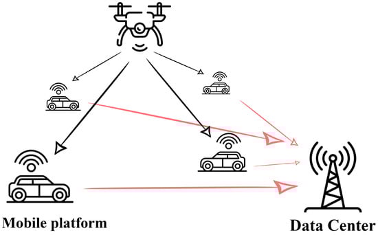
Figure 1.
Typical direction-finding system based on multiple mobile nodes organized as an IoT network.
In some cases, antennas should not be visually identifiable. For this purpose, they should be either small or similar in shape to a non-radiating object. Several small-size, multi-band or wideband antenna structures exist; however, most of them cover frequency ranges above the UHF band. They are generally multi-port structures, provide low-gain figures, and are still visible since they must be placed vertically [15,16]. Some low-profile antenna structures for UHF have also been proposed; however, only one dimension is made small [17,18,19], and lumped elements might be needed to match the input impedance [18].
Mimetic antennas [20,21] are essentially radiating structures that should fit into a given shape and size, as they cannot be visually identified. There are mainly two techniques to design mimetic radiators, i.e., either by masking generic antennas behind enclosures imitating air conditioners, fire sprinklers, exhausting pipes, etc. [22,23], or by exciting existing metal structures to radiate in a desired manner. The second technique is mostly used for HF and VHF communications and consists of inducing characteristic modes on a vehicle or ship body [24,25]. However, in some cases the antenna structure does not fall in any of the two categories listed above. As an example, the receiving antennas for mobile platforms in a direction-finding network as described before may have to look like a car luggage rack. For multiple-band or wideband operation, the antenna should provide optimal resonant frequencies, directivity, and gain figures for a given shape and size. Under such constraints, the only way to achieve optimal characteristics is to decide which parts of a fixed-shape structure should be made out of a conducting or insulating material [26]. Adjustments may lead to a large number of structures to be simulated; therefore, a selection among all possible configurations based on analyzing the potential resonant paths might help to find the optimal structure much faster than simulating all possible conductor–insulator combinations.
Part of some recent studies propose antenna design techniques based on machine learning. For instance, [27] demonstrates that even a limited number of simulation-based predictions, when strategically chosen, can effectively guide structural antenna optimization using machine learning. Similarly, [28,29,30,31] explore various learning algorithms (ANN, SVM, Random Forest, XGBoost), confirming that both model type and the number of predictions significantly influence the accuracy of VSWR and resonant frequency estimation. For the fine-tuning stage, [32] shows that scaling high-impact structural segments using Bayesian optimization leads to substantial performance gains. Complementarily, [33] illustrates how adjusting slot dimensions via support vector regression enables convergence toward target resonant behavior with minimal error. However, machine learning might not provide a significant error reduction without a large training set. In addition, existing databases do not include such fixed-shape structures; therefore, they have to be simulated prior to using any machine learning algorithm.
The main goal of this work is to propose a design methodology entirely based on physical analysis for periodic antenna structures of fixed shape and size, mimicking a non-radiating object. We propose a two-step procedure to optimize a luggage-rack-like antenna for three frequency bands centered on 433 MHz, 877.5 MHz, and 2.4 GHz. The first step consists of encoding three-segment combinations of conductor and dielectric on each rack bar. We then define a set of possible configurations by analyzing the potential resonant paths and keeping them fixed. We choose from among the simulated configurations the optimal one that minimizes an error figure, defined in terms of VSWR and resonant frequencies.
The second step of our procedure is fine-tuning based on scaling the segments with the highest impact on the error figure. The results clearly show that the final antenna structure approaches the target characteristics at an error of less than 5%.
2. Design Constraints and Methodology
The antenna should fit the shape of a 1 by 1.3 m luggage rack with fourteen equally spaced parallel bars (Figure 2). The gap between the antenna and the car roof acting as a ground should be kept at 5 cm, and the bar diameter at 1.5 cm.
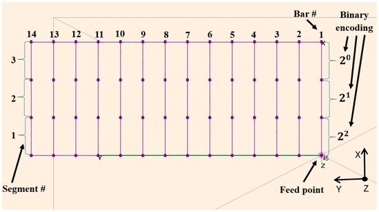
Figure 2.
Antenna shape with segment and bar referencing(# stands for number).
Each bar is considered to be made out of three equal-length segments; each of them can be either a conductor or a dielectric rod. To ease referencing, we encoded each bar by using a three-bit binary word, where 1 means conductor and 0 dielectric; for a simpler description, one can then convert the binary word into a decimal digit between 0 and 7. The most significant bit was considered on the excitation point side. As an example, for a bar with the first two segments (i.e., on the feed point side) made of conductor and the last one made of dielectric, the corresponding code word will be 110, i.e., 6 as a decimal digit.
The first step in designing the initial radiator structure is to ensure that there will at least be a current path close to an odd multiple of a quarter-wavelength (monopole mode resonance) for each frequency of interest. The configuration providing the closest approximation to a resonant length at each frequency of interest is that with bars #1, 3, 5, 6, and 8, providing each of them an open-ended segment, i.e., the corresponding code word should be either 4 or 5.
We calculated the length for any possible current path starting from the feed point, flowing through the long side of the frame next to the feed point, and eventually terminating on an open-ended segment of a transverse bar. The current path lengths were then compared to the wavelength in order to find the closest approximation to an odd number of quarter-wavelengths. The current paths corresponding to each resonant frequency are shown in Figure 3, and Table 1 shows the resonant path length in terms of wavelength.
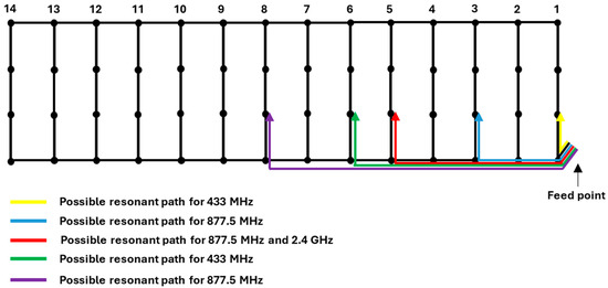
Figure 3.
Possible resonant current paths.

Table 1.
Possible resonant path length in terms of wavelength.
To better understand the resonant behavior of such a radiating structure, we simulated a reduced configuration (Figure 4), including the feed segment and the first three resonant paths as given in Figure 4 and Table 1.
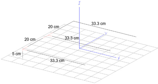
Figure 4.
Possible resonant structure.
The input reactance as a function of frequency (Figure 5) shows resonances at 485 MHz, 890 MHz, and 3400 MHz. A change in monotony can also be noted at 2390 MHz; although there is no null at that frequency, it could be seen as a resonant trend. Next, we show how completing the grid structure can bring the resonances closer to the target frequencies.
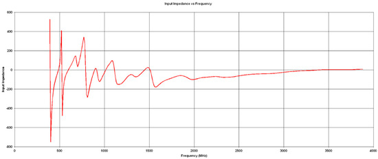
Figure 5.
Input reactance of the reduced radiating structure.
A total number of 84 configurations were characterized by using a MoM-based simulator for wire antennas by applying the resonant path constraint as described before.
In order to assess the overall performance of a given antenna structure, we have defined a normalized, multi-objective metric as follows:
where and are the computed resonant frequency for the n-th frequency band and the corresponding voltage standing wave ratio, respectively, while is denoted as the target resonant frequency. The metric weighs equally resonant frequencies and VSWR; it was set such that a VSWR figure below 2 has no effect on the error figure.
It should be emphasized that only configurations with a minimal gain of 2 dBi on each resonant frequency were retained. For each frequency band of operation, the resulting resonant frequency was chosen as corresponding to a minimum of VSWR within the range .
3. Antenna Design and Optimization
Table 2.
Possible configurations.
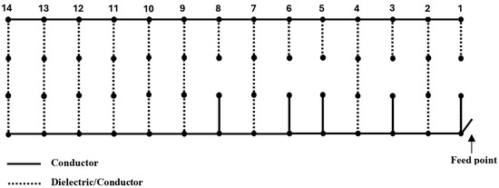
Figure 6.
Set of possible configurations.
More specifically, the 84 candidate structures were chosen among all possible configurations as follows.
Bars # 1, 3, 5, 6, and 8: These bars are part of the resonant paths and should therefore be open-ended, i.e., the corresponding codeword should be either 4 or 5. We choose to set them either all on 4 or all on 5. Rationale: The segments on the frame side opposite to the antenna input are fed through the rest of the radiating structure. They have less impact on the resonance since they are located at the end of the current path. For this reason, the number of combinations can be decimated as shown before.
Bars # 2, 4: They are both set on 0. Rationale: These bars next to the resonant paths are the closest to the feed point. For this reason, they should not perturb the current distribution.
Bar # 7: All possible combinations were assigned to the codeword for this bar, except the codeword 2 which would correspond to an insulated segment. Rationale: This bar is the first one after identifying at least one resonant path for each frequency of interest. It was therefore chosen as a tuning element.
Bar #9: The codeword was set on a fixed value, i.e., 7. Rationale: This bar bridges a current path length resonating close to all the frequencies of interest.
Bars # 10, 11 and 12: They were set on 1 or 6, but not all of them at the same time, i.e., the combinations 111 and 666 were excluded to avoid a high current imbalance between the frame sides. Rationale: These bars can act as fine-tuning elements since they are located at the end of the structure.
Bars # 13 and 14: The corresponding codeword was set on 6. Rationale: These are the most remote bars from the feed point. They are not supposed to significantly change the resonant frequencies; consequently, the number of combinations can be decimated in this manner.
The configuration with the bar sequence [5 0 5 0 5 5 4 5 7 1 6 1 6 6] (Figure 7) yields the lowest error figure computed using (1), i.e., ϵ = 14.69% along with a gain over 2 dBi on all resonant frequencies, and was therefore chosen as a reference for further optimization.
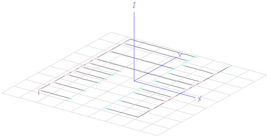
Figure 7.
Least-error configuration.
The least-error configuration was then simulated by using a MoM simulator (Table 3).
Table 3.
Optimal configuration: simulation.
Figure 8, Figure 9, Figure 10 and Figure 11 illustrate the VSWR variation for each frequency band considered, as well as the corresponding radiation patterns at the resonant frequency in the horizontal and vertical planes.

Figure 8.
VSWR variation for: (a) 433 MHz; (b) 877.5 MHz; (c) 2.4 GHz bands.
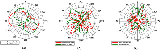
Figure 9.
Gain in the horizontal plane, horizontal and vertical polarization: (a) 433 MHz, θ = 26°; (b) 877.5 MHz, θ = −42°; (c) 2.4 GHz, θ = 53°.
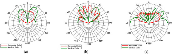
Figure 10.
Gain in the vertical plane for , horizontal and vertical polarization: (a) 433 MHz; (b) 877.5 MHz; (c) 2.4 GHz.
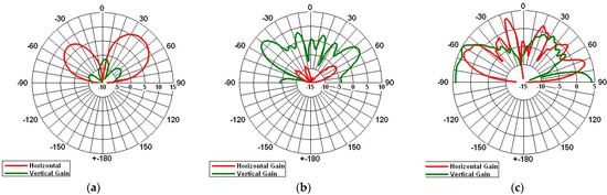
Figure 11.
Gain in the vertical plane for , horizontal and vertical polarization: (a) 433 MHz; (b) 877.5 MHz; (c) 2.4 GHz.
In order to further optimize the antenna performances and ensure resonance at the target frequencies, a detailed analysis of the current distribution along each segment was conducted. The study revealed that the feed segment plays a predominant role in achieving resonance at 2.4 GHz, whereas segment 1 of bar #1 has the most significant influence on the resonance at 433 MHz. Consequently, a fine-tuning approach based on segment scaling was applied as follows:
- (i)
- The feed segment was lengthened from 5 cm to 6.25 cm to shift the resonance closer to 2.4 GHz;
- (ii)
- Segment 1 of bar #1 was extended from 33 cm to 38 cm to provide resonance at 433 MHz.
It should be noted that the scaling factors can be different from the actual frequency ratios due to the complexity of the radiating structure. After fine-tuning, some parameters might slightly vary from those of the initial structure; however, the aim of the optimization is to minimize the error figure in (1).
Figure 12 illustrates the antenna structure after the fine-tuning and the current distributions at the frequencies of interest.
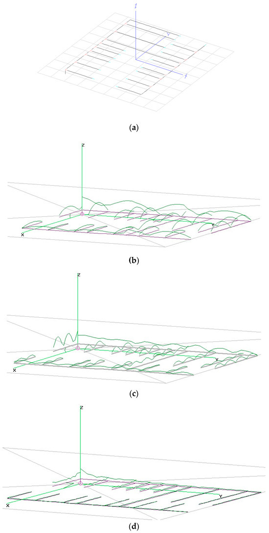
Figure 12.
Antenna structure after the fine-tuning: antenna model (a) and current distribution at 433 MHz (b), 877.5 MHz (c), and 2.4 GHz (d).
Figure 13 illustrates the VSWR variation for each frequency band for the optimal antenna structure. Table 4 shows the characteristics of the final design. Figure 14, Figure 15 and Figure 16 show the radiation patterns corresponding to the resonant frequency in the horizontal plane and vertical plane.
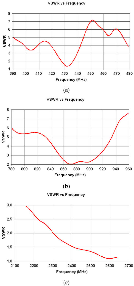
Figure 13.
VSWR variation for (a) 433 MHz; (b) 877.5 MHz; (c) 2.4 GHz bands.
Table 4.
Optimal configuration characteristics.
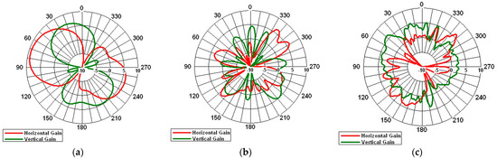
Figure 14.
Gain in the horizontal plane, horizontal and vertical polarization: (a) 433 MHz, θ = 26°; (b) 877.5 MHz, θ = 41°; (c) 2.4 GHz, θ = 50°.
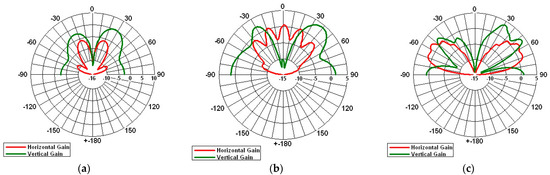
Figure 15.
Gain in the vertical plane for , horizontal and vertical polarization: (a) 433 MHz; (b) 877.5 MHz; (c) 2.4 GHz.
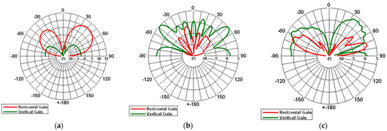
Figure 16.
Gain in the vertical plane for , horizontal and vertical polarization: (a) 433 MHz; (b) 877.5 MHz; (c) 2.4 GHz.
After performing the fine-tuning as shown before, the error figure as defined in (1) went down to 3.53%.
4. Experimental Results
The optimal antenna configuration was manufactured by using copper pipes for the conducting segments of the grid structure and for the excitation segment and PVC pipes for the dielectric segments and for supporting the other three corners of the frame when mounted on top of a car. The copper pipes were cut at a tolerance of 1 mm, and the PVC pipes overlap the copper segments at the joints by approximately 1 cm to provide good mechanical strength.
The antenna was measured in an anechoic chamber (Figure 17). A metal shield was placed on the floor of the chamber; the antenna therefore operates under infinite-like ground plane conditions.
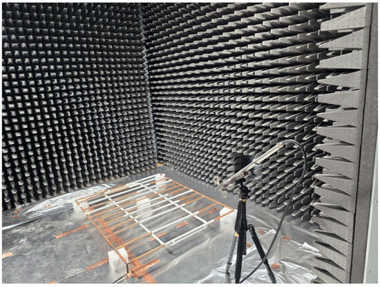
Figure 17.
Experimental model.
Firstly, we measured the magnitude of the reflection coefficient at the antenna input to make sure that resonance is present at the required frequencies. Then, we placed a calibrated biconical dipole 1.14 m away from the antenna under testing in order to measure the realized gain at and in vertical polarization (Figure 18). As shown in Figure 16, the polarization is mixed since part of the structure consists of orthogonal radiators.
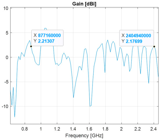
Figure 18.
Gain variation.
The probe antenna operates between 600 MHz and 3 GHz. We highlighted on the diagram the gain figures at 877 MHz and 2.4 GHz, which are close to the results presented in Figure 16.
It should be emphasized that in the application under consideration, pattern diagrams are less important since the IoT system includes several mobile platforms; if the target does not fall in a null direction for at least three of them, then the system is able to locate it.
Figure 19 shows rather good agreement between simulated and measured results for all three frequencies of interest. Discrepancies between simulated and measured results occur especially at high frequencies due to the limitations of the wire antenna simulator for modeling the excitation, i.e., locally applied electric field versus real coaxial connectors.
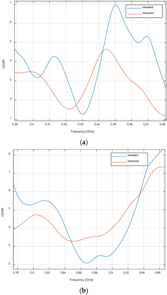
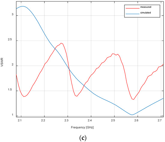
Figure 19.
Simulated vs. measured VSWR for (a) 433 MHz; (b) 877.5 MHz; (c) 2.4 GHz bands.
5. Conclusions
This work presents a method to generate a multi-band antenna, based on a fixed-shape structure imitating a car luggage rack.
The first step was to define a set of possible configurations based on physical analysis of the potential resonant paths. While a brute-force approach would require 814 = 4,398,046,511,104 full-wave simulations, our method dramatically reduces the computing time by performing only 84 simulations.
The next step was to further reduce the error figure by scaling the segment dimensions to fine-tune the resonant frequencies, allowing for better control of the antenna multi-band operation. Size scaling targeted the segments virtually, leading to the higher shift in resonant frequency, and the final error figure was thus made as low as 3.53%. The antenna was then manufactured and measured; the final design provides good gain and VSWR figures over almost all the frequency ranges of interest.
Further enhancements can be achieved by refining the antenna design parameters, e.g., the number of segments per bar. Increasing the number of segments per bar would provide a finer mesh in the optimization process, potentially leading to superior configurations. Yet, it also leads to a larger number of configurations and, eventually, to a longer computing time.
It should be emphasized that, in the current development stage, we focused on the design procedure rather than on practical configurations. The antenna was therefore designed and characterized over an infinite ground plane, allowing for fast simulations. For operating over a real vehicle body, design, simulation, and measurements should be performed accordingly.
Funding
This research was funded by Constanta Maritime University under the project MAREHC, a grant of the Romanian Ministry of Research, Innovation and Digitalization, project number PNRR-C9-I8-760111/23.05.2023, code CF 48/14.11.2022, within PNRR.
Data Availability Statement
Ongoing research project requiring confidential data status.
Acknowledgments
The author is grateful to the members of his team who kindly supported him in achieving the results presented this work.
Conflicts of Interest
The author declares no conflicts of interest.
Abbreviations
The following abbreviations are used in this manuscript:
| ANN | Artificial Neural Network |
| UHF | Ultra-High Frequency |
| SVM | Support Vector Machine |
| MoM | Method of Moments |
| VSWR | Voltage Standing Wave Ratio |
References
- Khan, J.; Kiani, G. Parametric study of microstrip patch antenna on LCP substrate for 70 GHz applications. In Proceedings of the 2015 IEEE 4th Asia-Pacific Conference on Antennas and Propagation (APCAP), Bali, Indonesia, 30 June–3 July 2015; pp. 554–555. [Google Scholar] [CrossRef]
- Shariar, F.; Hossain, M.F. Design and Analysis of a Triple Band Microstrip Patch Antenna for Wireless Applications. In Proceedings of the 2023 6th International Conference on Electrical Information and Communication Technology (EICT), Khulna, Bangladesh, 7–9 December 2023; pp. 1–6. [Google Scholar] [CrossRef]
- Constantin, A.; Ifrim, G.; Tamas, R.D. Innovative Dual-Band Antenna for Reliable LoRa IoT Connectivity. In Proceedings of the 2024 Advanced Topics on Measurement and Simulation (ATOMS), Constanta, Romania, 28–30 August 2024; pp. 81–84. [Google Scholar] [CrossRef]
- Heiman, C.-A.; Constantin, A.; Pastorcici, M.; Tamas, R.D. Wideband Circularly Polarized FSS-Horn Antennas. In Proceedings of the 2023 IEEE-APS Topical Conference on Antennas and Propagation in Wireless Communications (APWC), Venice, Italy, 9–13 October 2023; pp. 35–37. [Google Scholar] [CrossRef]
- Liu, J.; Yang, Y.; Li, N.; Xie, K. Optimization of Broadband Patch Antenna Based on Mind Evolutionary Algorithm. In Proceedings of the 2009 International Conference on Networks Security, Wireless Communications and Trusted Computing, Wuhan, China, 25–26 April 2009; pp. 361–364. [Google Scholar] [CrossRef]
- Bucuci, S.; Constantin, A.; Paun, M.; Pastorcici, M.N.; Tamas, R.D.; Danisor, A.; Constantinescu, R. A Compact Monopole Antenna for Underwater Acoustic Monitoring Beacons. Sensors 2022, 22, 8392. [Google Scholar] [CrossRef] [PubMed]
- Yusuf, A.N.A.; Purnamasari, P.D.; Zulkifli, F.Y. A Comparative Analysis of Machine Learning Algorithms for Predicting the Dimensions of Rectangular Microstrip Antennas. In Proceedings of the 2023 IEEE International Symposium on Antennas and Propagation (ISAP), Kuala Lumpur, Malaysia, 30 October–2 November 2023; pp. 1–2. [Google Scholar] [CrossRef]
- Gampala, G.; Reddy, C.J. Fast and Intelligent Antenna Design Optimization using Machine Learning. In Proceedings of the 2020 International Applied Computational Electromagnetics Society Symposium (ACES), Monterey, CA, USA, 27–31 July 2020; pp. 1–2. [Google Scholar] [CrossRef]
- Misilmani, H.M.E.; Naous, T. Machine Learning in Antenna Design: An Overview on Machine Learning Concept and Algorithms. In Proceedings of the 2019 International Conference on High Performance Computing & Simulation (HPCS), Dublin, Ireland, 15–19 July 2019; pp. 600–607. [Google Scholar] [CrossRef]
- Ahmad, T.; Li, X.J.; Ashfaq, M.; Savva, M.; Ioannou, I.; Vassiliou, V. Location-enabled IoT (LE-IoT): Indoor Localization for IoT Environments using Machine Learning. In Proceedings of the 2024 20th International Conference on Distributed Computing in Smart Systems and the Internet of Things (DCOSS-IoT), Abu Dhabi, United Arab Emirates, 29 April–1 May 2024. [Google Scholar] [CrossRef]
- Jahagirdar, S.; Ghatak, A.; Kumar, A.A. WiFi based Indoor Positioning System using Machine Learning and Multi-Node Triangulation Algorithms. In Proceedings of the 2020 11th International Conference on Computing, Communication and Networking Technologies (ICCCNT), Kharagpur, India, 1–3 July 2020; pp. 1–6. [Google Scholar] [CrossRef]
- Chiper, F.-L.; Martian, A.; Vladeanu, C.; Marghescu, I.; Craciunescu, R.; Fratu, O. Drone Detection and Defense Systems: Survey and a Software-Defined Radio-Based Solution. Sensors 2022, 22, 1453. [Google Scholar] [CrossRef] [PubMed]
- Famili, A.; Stavrou, A.; Wang, H.; Park, J.-M.; Gerdes, R. Securing Your Airspace: Detection of Drones Trespassing Protected Areas. Sensors 2024, 24, 2028. [Google Scholar] [CrossRef] [PubMed]
- Łukasiewicz, J.; Kobaszyńska-Twardowska, A. Proposed method for building an anti-drone system for the protection of facilities important for state security. Secur. Def. Q. 2022, 39, 88–107. [Google Scholar] [CrossRef]
- Hua, Y.; Huang, L.; Lu, Y. A Compact 3-Port Multiband Antenna for V2X Communication. In Proceedings of the 2017 IEEE International Symposium on Antennas and Propagation & USNC/URSI National Radio Science Meeting, San Diego, CA, USA, 9–14 July 2017; pp. 639–640. [Google Scholar] [CrossRef]
- Mousavi, P. Multiband Multipolarization Integrated Monopole Slots Antenna for Vehicular Telematics Applications. IEEE Trans. Antennas Propag. 2011, 59, 3123–3127. [Google Scholar] [CrossRef]
- Mohamed-Hicho, N.M.; Antonino-Daviu, E.; Cabedo-Fabrés, M.; Ferrando-Bataller, M. A Novel Low-Profile High-Gain UHF Antenna Using High-Impedance Surfaces. IEEE Antennas Wirel. Propag. Lett. 2015, 14, 1014–1017. [Google Scholar] [CrossRef]
- Wu, W.; Guan, B. A low-profile broadband UHF base station antenna based on lumped-element matching network. In Proceedings of the 2016 11th International Symposium on Antennas, Propagation and EM Theory (ISAPE), Guilin, China, 18–21 October 2016; pp. 9–12. [Google Scholar] [CrossRef]
- Keum, K.-S.; Park, Y.-M.; Choi, J.-H. A Low-Profile Wideband Monocone Antenna Using Bent Shorting Strips. Appl. Sci. 2019, 9, 1896. [Google Scholar] [CrossRef]
- Alieldin, A.; Huang, Y.; Stanley, M.; Joseph, S.; Jia, T.; Elhouni, F. A Camouflage Antenna Array Integrated with a Street Lamp for 5G Picocell Base Stations. In Proceedings of the 2019 13th European Conference on Antennas and Propagation (EuCAP), Krakow, Poland, 31 March–5 April 2019; pp. 1–4. Available online: https://ieeexplore.ieee.org/document/8739400 (accessed on 12 March 2025).
- Sanz-Izquierdo, B.; Huang, F.; Batchelor, J.C. Small size wearable button antenna. In Proceedings of the 2006 First European Conference on Antennas and Propagation, Nice, France, 6–10 November 2006; pp. 1–4. [Google Scholar] [CrossRef]
- Alieldin, A.; El-Akhdar, A.M.; Eldamak, A.R.; Abounemra, A.M.E.; Darwish, M. A Camouflage Fire Sprinkler Antenna for Indoor Sub-6 GHz 5G and WiFi Applications. In Proceedings of the 2025 International Telecommunications Conference (ITC-Egypt), Cairo, Egypt, 28–31 July 2025; pp. 1–4. [Google Scholar] [CrossRef]
- Кн-Будинжиниринг, M. Camouflage Antenna Catalog. Available online: https://www.academia.edu/37674623/_Camouflage_Antenna_Catalog (accessed on 22 October 2025).
- Shih, T.-Y.; Behdad, N. Design of vehicle-mounted, compact VHF antennas using characteristic mode theory. In Proceedings of the 2017 11th European Conference on Antennas and Propagation (EUCAP), Paris, France, 19–24 March 2017; pp. 1765–1768. [Google Scholar] [CrossRef]
- Yeung, S.H.; Wang, C.-F. Characteristic mode theory for practical HF antenna design. In Proceedings of the 12th European Conference on Antennas and Propagation (EuCAP 2018), London, UK, 9–13 April 2018; pp. 1–4. [Google Scholar] [CrossRef]
- Heiman, A.; Tamas, R.D. Transforming Linear to Circular Polarization on Horn Antennas by Using Multiple-Layer Frequency Selective Surfaces. Sensors 2022, 22, 7838. [Google Scholar] [CrossRef]
- Bazgir, M.; Sheikhi, A.; Dowlatshahi, M. Resonance frequency prediction of dielectric antennas for liquid sensing via support vector regression. Sci. Rep. 2024, 14, 31410. [Google Scholar] [CrossRef] [PubMed]
- Singh, O.; Bharamagoudra, M.; Gupta, H.; Dwivedi, A.; Ranjan, P.; Sharma, A. Microstrip line fed dielectric resonator antenna optimization using machine learning algorithms. Sādhanā 2022, 47, 226. [Google Scholar] [CrossRef]
- Heiman, A.; Tamas, R.D. Neural Network-Based Predictive Design of FSS Structures for Satellite Antenna Performance Enhancement. In Proceedings of the IEEE International Conference on Antenna Measurements and Applications (CAMA)-Special Sessions: SPS16 New Technologies and Methodologies for Antenna Design, Antibes, France, 18–20 November 2025. [Google Scholar]
- Constantin, A.; Tamas, R.D. A Multi-Band AI-Miniaturized Patch Antenna for Environmental Monitoring. In Proceedings of the IEEE International Conference on Antenna Measurements and Applications (CAMA)-Special Sessions: SPS16 New Technologies and Methodologies for Antenna Design, Antibes, France, 18–20 November 2025. [Google Scholar]
- Ranjan, P.; Gupta, H.; Sharma, A.; Yadav, S.; Potrebićc, M. Investigation and Optimization of Dielectric Resonator MIMO Antenna Using Machine Learning Approach; Springer Nature: Singapore, 2022; pp. 645–655. [Google Scholar] [CrossRef]
- Huang, C.-H.; Ali, A.; Hsu, C.-C.; Tsao, H.-H. Enhanced Antenna Design Through Hyper Parameter Optimization of Diverse Machine Learning Models Using Bayesian Optimization. Res. Sq. Prepr. 2024. [Google Scholar] [CrossRef]
- Khan, T.; Roy, C. Prediction of slot-position and slot-size of a microstrip antenna using support vector regression. Int. J. RF Microw. Comput.-Aided Eng. 2018, 29, e21623. [Google Scholar] [CrossRef]


Disclaimer/Publisher’s Note: The statements, opinions and data contained in all publications are solely those of the individual author(s) and contributor(s) and not of MDPI and/or the editor(s). MDPI and/or the editor(s) disclaim responsibility for any injury to people or property resulting from any ideas, methods, instructions or products referred to in the content. |
© 2025 by the author. Licensee MDPI, Basel, Switzerland. This article is an open access article distributed under the terms and conditions of the Creative Commons Attribution (CC BY) license (https://creativecommons.org/licenses/by/4.0/).