Abstract
The increasing integration of distributed renewable energy sources into distribution networks results in significant voltage regulation challenges. To address these challenges, we introduce a novel data-driven approach for voltage regulation that utilizes predictive control mechanisms, specifically data-enabled predictive control (DeePC). This method exploits the capabilities of photovoltaic (PV) inverters and battery energy storage systems (BESS) to manage bus voltages within the distribution network. Unlike traditional model-based approaches that require a precise physical model of the network, the DeePC algorithm operates optimally by relying solely on historical data to predict and adjust bus voltages. By employing the DeePC algorithm, the proposed controller maintains voltage profiles and the state of charge (SoC) of BESSs within operational thresholds in an optimal and robust manner. To further reduce the computational complexity, a reformulation of DeePC is developed using scoring functions, where the DeePC algorithm is efficiently approximated via differentiable convex programming. We validate our approach through simulations on the IEEE 34-bus test system, demonstrating its efficiency in maintaining desired voltage levels without the need for a detailed physical system model.
1. Introduction
The increasing integration of distributed generation (DG) into distribution networks (DNs) has introduced significant challenges related to voltage regulation, particularly due to the reverse power flow caused by the high penetration of PV systems. These challenges primarily manifest as voltage fluctuations and voltage violations, complicating the operational management of DNs [1]. To mitigate these challenges, voltage regulation strategies have drawn increasing attention, driven by elevated levels of PV penetration. Various approaches have been explored, including PV generation curtailment [2], inverter-based control strategies [3,4], and the integration of an energy storage system (ESS) [5]. In recent years, BESSs have emerged as a promising solution to enhance voltage regulation in distribution networks, offering a flexible and efficient approach to addressing voltage fluctuations [6]. Given the variability associated with distributed energy resources (DERs), effectively coordinating systems like PV and BESS to deliver precise control actions poses a significant challenge in voltage management.
In the literature, various strategies have been proposed to mitigate the voltage impacts of PV generation. In [7], a charging/discharging strategy is designed for ESS integrated with PV generation. A droop-based control approach that combines ESS with the reactive capacity of PV generation to improve voltage profiles is presented in [8]. In [6], a distributed control scheme leveraging PV generation is introduced. A combination of localized and distributed algorithms for regulating voltage magnitudes within a specified range while minimizing the output of controllable devices is detailed in [9]. The weighted regulation method in [10] adjusts the charge/discharge rates of BESS based on their capacities. In [6], a coordinated control strategy for BESS is proposed, integrating distributed and localized control methodologies.
Although the previously discussed control strategies effectively facilitate voltage regulation, their performance depends on comprehensive network modeling with complete physical information. This reliance can be problematic, as obtaining and maintaining such detailed models is challenging—especially in dynamic environments with high renewable energy penetration. Consequently, the effectiveness of model-based design strategies is substantially undermined. As reported in [11], discrepancies between the actual system model and the design model can lead to performance degradation or even significant deterioration of control performance.
To address these challenges, data-driven methods have emerged as promising approaches for designing voltage control strategies in DNs. These methods are broadly categorized into two paradigms: direct data-driven control and machine learning-based control. Recent advances in machine learning have introduced innovative solutions to traditional voltage regulation problems [12]. For example, Reference [13] employs a Monte Carlo tree search-based reinforcement learning (MCTS-RL) framework to coordinate PV generation and BESS for voltage regulation. Similarly, Reference [14] proposes a deep deterministic policy gradient (DDPG)-based online scheduling algorithm to optimize PV-BESS dispatch by learning operational patterns of PV generation and grid conditions. To enhance adaptability during unexpected topology changes, Reference [15] introduces a multi-task soft actor-critic (MT-SAC) deep reinforcement learning (DRL) approach for voltage regulation via PV control. Further advancing this field, Reference [16] develops a physics-model-free dual-time-scale voltage control framework, where the scheduling of PV generation across multiple sub-networks is formulated as a Markov game and solved using a multi-agent soft actor-critic (MASAC) algorithm. In this approach, each sub-network operates as an autonomous intelligent agent.
However, machine learning-based control methods inherently depend on extensive offline datasets for initial model training. These approaches often face challenges in computational efficiency, prolonged training durations, and limited adaptability to evolving system conditions. A critical limitation arises when network topology changes render existing models obsolete, thereby requiring extensive data recollections and computationally intensive retraining processes. Such procedures introduce significant time delays and operational costs while compromising control performance in dynamic environments [12,17,18].
In contrast, direct data-driven methods rooted in behavioral system theory—such as data-enabled predictive control (DeePC)—eliminate the need for system identification by directly synthesizing control strategies from limited historical data. DeePC operates by constructing a nonparametric model using measured system trajectories, contingent on the input signals satisfying persistent excitation criteria. While conventional DeePC frameworks bypass parametric modeling and derive optimal control policies from raw datasets, their reliance on large-scale data introduces a critical limitation: computational complexity scales exponentially with the dimensionality of input–output data, posing challenges for high-dimensional or real-time systems [19,20,21]. To mitigate this issue, we propose a reformulated DeePC framework that integrates scoring functions and employs differentiable convex programming to approximate the original optimization problem efficiently.
In this study, we propose a novel control strategy for BESSs aimed at voltage regulation in distribution networks with high PV penetration. This strategy is based on a direct data-driven algorithm. The principal contributions of this article are as follows:
- 1.
- The proposed control method is entirely data-driven, eliminating the need for specific physical parameters. Instead, they construct a nonparametric model of the system based on historical data. By continuously updating and iterating the input–output data, the method achieves highly accurate predictions of future input–output data.
- 2.
- Based on the scoring functions, we propose a reformulation of DeePC that introduces a novel perspective for data-enabled approaches. The score functions are parameterized as a differentiable convex program, enabling efficient approximation and enhancing the applicability of DeePC.
- 3.
- The proposed BESS control strategy aims to regulate voltage in distribution networks with high levels of PV. This strategy ensures that the voltage at each bus in the distribution network remains within permissible limits, preventing overvoltage or undervoltage conditions that could compromise the stability of the system.
- 4.
- The IEEE 34-bus test is employed to demonstrate the effectiveness of the proposed data-driven control scheme, and the control performance is comparable with the model-based scheme.
Compared to existing data-driven methods such as reinforcement learning, the proposed DeePC-based approach does not require extensive offline training or retraining when system conditions change. Unlike model-based methods, it eliminates the need for accurate network parameters. Furthermore, the introduction of a differentiable convex programming-based approximation significantly reduces online computational burden, making it more suitable for real-time voltage control in large-scale distribution networks.
This paper extends our previous study [22] in the following three aspects. Firstly, it extends the data-driven control approach originally proposed for small-networked microgrid systems (NMG) in [22] to large DNs. Secondly, in contrast to [22], this work not only regulates PV generation but also incorporates BESSs for voltage regulation. Last, this work employs a reformulation of DeePC instead of the general version of DeePC presented in [22].
The rest of the article is organized as follows: Section 2 provides the system model. Section 3 presents an overview of the DeePC algorithm and a reformulation of DeePC. In Section 4, a detailed discussion on the DeePC-based voltage control scheme is provided. The case studies are presented in Section 5, followed by the conclusions presented in Section 6.
2. Network Description
In this section, we introduce the DN model used to implement the DeePC method. Consider a DN consisting of N + 1 buses, represented by the set Na:= {0, 1 …, N}, with distribution lines defined by the set Ea:= {(s, t)} ⊂ Na × Na. A typical example is illustrated in Figure 1. In the DN model, the bus indexed as zero, known as the point of common coupling (PCC), typically located at the distribution substation, serves as the voltage reference point. Each bus is equipped with a PV for local power generation. The voltage magnitude, active power injection, and reactive power injection at each bus are denoted by Vs, Ps, and Qs ∈ ℝn respectively, measured in per unit (p.u.). For each line (s, t)∈ Ea, Rst and Xst denote the line resistance and reactance, while Rst and Qst denote the net active and reactive power injected from bus s to bus t, respectively. The DistFlow equations [17], used to model power injection and voltage for every line (s, t)∈ Ea, are given as follows:
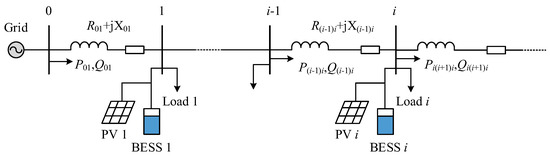
Figure 1.
Structure of the distribution network.
The DistFlow equations can be linearized as follows by assuming that: (a) line losses are negligible compared to power flow and (b) the voltage profile is relatively flat (i.e., ) [17]:
which can be reformulated in a compact form as:
where V0 ∈ ℝn is fixed to be the unit, and matrices N*, M* ∈ n represent sensitivity matrices derived from specific system parameters
where both N* and M* are positive definite matrices (PD) [23]. The total injected active power is decomposed into two constituent parts as pc + pe, where represents the controllable component (e.g., PV generation, BESS), and denotes the exogenous component (e.g., uncontrollable loads). The total injected reactive power is defined the same as the active power by following the same decomposition procedure. We define N*P + M*Q + V01n∈ ℝn, yielding:
The objective of voltage control in DNs is to maintain voltage levels within acceptable limits by regulating both reactive and active power provided by control resources given the voltage condition . The voltage control problem can therefore be expressed as
Defining Ꞷe(t) = (t)−(t − 1), we obtain the following control system:
Within this framework, the control objective at time t is to regulate bus voltages within a safe operational range by adjusting the active power injections pc from controllable resources. When the sampling interval Δt is sufficiently short (e.g., minute-scale), voltage deviations caused by exogenous factors such as uncontrollable generation or load variations can be approximated as quasi-static, i.e., Ꞷe(t) = 0. This assumption holds because slow-varying exogenous disturbances exhibit negligible variation over short time horizons.
3. Proposed Control Scheme
Based on the linearized DistFlow model in (7), the control problem is constructed as follows, where the objective is minimize the control efforts of PV and BESS while satisfying the system model introduced in Section 2, control limits, and voltage limits:
subject to
where Qg and Pg represent the reactive and active power generated by the PV systems and BESSs, respectively, with μ denoting the voltage set-points. The matrices Ξ, R and Ψ are positive definite. Vectors ε and δ serve as slack variables to soften the hard voltage constraints with Vmin and Vmax defining the voltage limits. A sufficiently large penalty parameter κ is chosen to enforce constraint satisfaction in the optimization problem. The reactive power output of the PV generation is determined by its rated capacity S and the corresponding active power Pv. The SoC at a given time instant t, denoted as SoC(t), is defined as the ratio of the current available capacity to the maximum allowable capacity of the BESS under the same conditions. SoCmax indicates the maximum energy storage capacity of the BESSs, while and denote the maximum charging and discharging power, respectively. The charge per unit limits, ρmin and ρmax, represent the minimum and maximum allowable SoC levels. The time step is represented by ∆t, while χ accounts for the efficiency of the BESSs.
Given the challenges in accurately obtaining the topology and line parameters of the DNs—i.e., the sensitivity matrices N* and M* in (4) are often unknown in practice—it becomes difficult to directly address the voltage control problem using model-based approaches that rely on precise physical representations. Consequently, it is essential to explore alternative methods for constructing a voltage control model based on system input–output data when N* and M* are unavailable. To address these challenges, the DeePC control framework is introduced in subsequent sections. This framework enables voltage control and optimization in DNs without requiring detailed physical models. Specifically, the DeePC algorithm is formulated to solve the control problem (8a)–(8k) while bypassing the need for precise network parameters.
The application of DeePC in this work is based on the following criteria: (i) the unavailability or inaccuracy of physical network models; (ii) the presence of time-varying dynamics due to high renewable penetration; (iii) the availability of sufficient historical input–output data; (iv) the ability to ensure persistent excitation through controlled perturbations; and (v) the need for real-time, scalable control. These factors make DeePC a suitable candidate for data-driven voltage regulation in active distribution networks. Furthermore, the proposed approximation via differentiable convex programming enables efficient online implementation, addressing the scalability challenge of standard DeePC in large-scale systems.
4. Overview of DeePC Algorithm
This section delineates that the dynamics of linear system can be learned directly from trajectories, obviating the necessity for a system model.
4.1. Data-Driven System Representation
Consider a controllable and observable linear time-invariant (LTI) system
where x(t) ∈ ℝn, u(t) ∈ ℝm, y(t) ∈ ℝp and d(t) ∈ ℝq represent the state, input vector, output vector, and external input variables, respectively, at discrete time steps t ∈ ℤ>0. In this study, the system state and output are defined as voltage measurements, i.e., x(t) = y(t) = V(t), while u(t) represents the changes in active and reactive power injection. The term d(t) = we(t) accounts for the voltage fluctuations resulting from the unregulated operation of loads and PV generation. The system matrices are specified as A = C = Zd = I, B = [N*; M*] and D = 0.
As previously discussed, solving the control problem (8a)–(8k) presents a significant challenge due to the lack of sufficiently accurate physical parameters for ADNs. Specifically, matrix B (refer to (9)), which depends on the physical model, remains indeterminate, making it impractical to directly implement optimal voltage control using traditional model-based approaches. Unlike conventional system theory, which requires explicit system parameterization, behavioral control theory relies solely on measured input–output data to construct a data-driven representation of the system’s signal space. This challenge can be addressed by formulating a data-driven model based on raw measurement data, thereby circumventing the need for an explicit physical model.
In the data-driven approach, we impose the following assumption: d(t) = we(t), which defines a signal that remains consistently predictable and satisfies d(t) = d(t + 1), indicating that the voltage variation between successive time steps is constant. Specifically, this implies that the uncontrollable voltage, , remains constant between successive time steps. The assumption is reasonable when the sampling interval is sufficiently short, ensuring minimal fluctuations in uncontrollable voltage sources. Based on the above assumption, we derive the following system model:
where the parametric matrix B in (9) is unknown, behavioral system theory enables the replacement of traditional LTI models with nonparametric data-driven representations [18]. Let u = col(u0, u1, …) denote a persistently exciting input trajectory of length T. The Hankel matrix, a cornerstone of behavioral theory, organizes this data into a structured matrix for system identification. For a user-defined horizon L ∈ ℤ>0, the input Hankel matrix is constructed as:
where each column of the input Hankel matrix HL(ud) ∈ ℝmL×(T−L+1) represents a length-L subsequence of the persistently exciting input trajectory ud = col(u0,u1, …, uT−1). Similarly, the output Hankel matrix is defined analogously using measured outputs yd = col(y0, y1, …, yT−1). Let Tini, Tf ∈ ℤ>0 denote the past and future horizons, respectively, with L = Tini + Tf. The Hankel matrices are partitioned into past and future components:
Here, Up and Yp represent the past components of the Hankel matrices, corresponding to the first Tini time steps, while Uf and Yf denote the future components associated with the next Tf time steps. If the Hankel matrix has full row rank, i.e., rank() = mL, then the input signal sequence u is defined as an L-order continuously exciting sequence. To ensure that maintains full row rank, the length of the initial trajectory T must satisfy the lower bound condition T ≥ (m + 1)L−1 [24]. This condition ensures the Hankel matrix spans the full input–output behavior space of the LTI system . Assume that the precollected input ud is persistently exciting of order Tini + Tf + n(), where n() denotes the system lag. Willems’ fundamental lemma [24] guarantees that any valid future trajectory col(u,y) can be expressed as a linear combination of the Hankel matrix columns. Given the current time t, a trajectory col(uini, yini, u, y) is generated from the system, implying the existence of a vector g ∈ ℝT−L+1 [25]:
This relationship forms the foundation of the DeePC framework. In this framework, the future behavior of the system is effectively predicted using historical input–output data, thus eliminating the need for an explicit system model. The parameter g serves as the decision variable spanning the precollected data, while u and y represent the predicted control inputs and outputs, respectively. The matrix [Up⊤ Yp⊤ Uf⊤ Yf⊤]⊤, constructed from historical input–output data, ensures that the optimization process remains purely data-driven. The trajectory wini = col(uini, yini) is generated from the latest input–output measurements and is used to estimate the system’s initial conditions in real time. By solving yini =Ypg and uini =Upg in (13), the decision variable g is determined, which subsequently enables the prediction of the system’s output via y =Yfg. Figure 2 provides a simplified schematic of the DeePC formulation as presented in (13). It illustrates how the vector g selects elements from the historical trajectory library [Up⊤ Yp⊤ Uf⊤ Yf⊤]⊤ to ensure alignment and consistency with both the initialized and future trajectories col(uini, yini, u, y). The DeePC based optimization problem can be formulated as follows:
where the Hankel matrices and are constructed from pre-collected input–output trajectories wd = col(ud, yd) ∈ T, where T denotes the system’s behavior over T time steps. The vector wini = col(uini, yini) ∈ represents the most recent Tini input–output measurements, while u∈ℝm and y∈ℝn denote future control inputs and predicted outputs over a horizon Tf. Let define the reference voltage trajectory. The quadratic cost function is weighted by Ξ ∈ ℝn×n (output tracking error) and R ∈ ℝm×m (control effort).
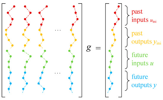
Figure 2.
Schematic illustration of the DeePC formulation of (13).
Considering the presence of uncertainties and noise, we introduce slack variables and to soften and relax the corresponding constraints [25,26,27], ensuring feasibility and robustness in the presence of uncertainties. The modified DeePC based optimization problem, incorporating these slack variables, is formulated as follows:
where the regularization term h(g) = is included to mitigate the effects of noise and inaccuracies in data, thereby enhancing the robustness of the control strategy in nonlinear computations. The regularization parameters , , ∈ ℝ>0 penalize the slack variables and the regularization term, ensuring a smooth and stable input trajectory.
4.2. Approximation of DeePC
The DeePC framework constructs nonparametric system representations directly from input–output trajectories, bypassing explicit physical modeling while capturing dynamic system behavior through historical data. By embedding implicit operational patterns from measured trajectories, DeePC enhances control flexibility and robustness in uncertain grid environments. However, its computational complexity scales exponentially with the dimensionality of the data matrix M ∈ ℝ(m+p)L×(T−L+1), where L = Tini + Tf is the total prediction horizon. This arises because the decision variable g ∈ ℝT−L+1 grows linearly with the dataset size T, rendering real-time optimization intractable for large-scale distribution networks.
To address this limitation, we propose a learning-based approximate DeePC framework that replaces the full-data optimization with a parametric surrogate model [28]. This model is trained offline to approximate the optimal control policy using supervised learning on historical DeePC solutions, thereby reducing online computation to a low-dimensional function evaluation.
Consider the predicted I/O trajectory sequence as τ = col(u,y), where u ∈ ℝmL and y ∈ ℝpL. To balance computational efficiency with control performance, we reformulate the DeePC optimization (16) by decoupling the objective into two components:
where the objective function is defined as follows:
and r r ⊗ 1L, R R ⊗ IL, Ξ Ξ ⊗ IL, τini col(uini, yini), Fini is a selection matrix employed to extract the initial trajectory τini from the full I/O sequenc τ, is the augmented Hankel matrix which encodes the historical data constraints for predictive modeling. denotes the indication function. In the , “×” means Cartesian power. By employing an approximate form of the score function , we reconstruct the score function and reformulate the optimization problem. The new formulation seeks to balance computational efficiency with control performance while ensuring robust trajectory predictions. Thus, the modified control problem is given by:
Our proposed approximation goal is to ensure that the control input (i.e., the optimal solution to the learning problem ) closely matches the solution obtained from the true scoring function . To achieve this, we define the learning objective as minimizing the error between the proximal operators of the approximate scoring function and the true scoring function. Figure 3 illustrates the overall framework, depicting how the approximation process refines control performance while maintaining computational efficiency.
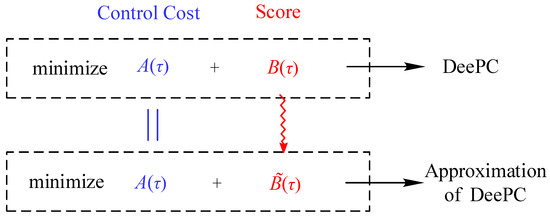
Figure 3.
Schematic illustration of the overall framework.
The proximal operator [29] of is defined as:
The optimal solution of (20) can be determined equivalently by reformulating the approximation operator of A and the scoring function in terms of operator splitting techniques. Given an appropriate formulation of the operator, the optimal solution can be efficiently computed. Based on differentiable convex programming, the approximate scoring function can be expressed as:
where is obtained through convex optimization with learnable parameters , , and . To achieve the learning objective, i.e., ensuring that ≈ , the differentiable convex program is trained using a gradient-based approach to iteratively update the parameters , , and .
Let , = , = −I. Under these conditions, is equivalent to . Based on (20), we derive the following results:
To solve (22) and compute the gradient of the learned parameters , , and with respect to , we employ an unrolling-based approach [30]. Specifically, the Douglas-Rachford Splitting (DRS) method [31] is utilized to iteratively solve (22) using the following process:
where , are auxiliary variables, = [ ], and is defined as:
Here, is the i-th element of . Figure 4 shows the unrolled DRS iterations Illustration.
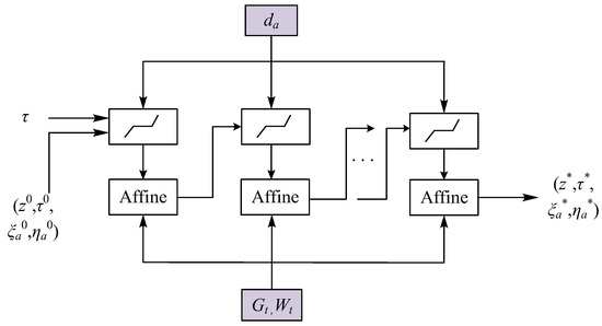
Figure 4.
Schematic illustration of the unrolled DRS iterations.
During the offline training phase, the internal optimization problem of approximating the scoring function is reformulated as a microscopic computational module using algorithm unrolling. Specifically, the DRS iterative process in (23) is expanded into a sequence of microscopic network layers, as illustrated in Figure 4. This transformation enables the utilization of existing deep learning frameworks to train the learning parameters , , and , ensuring that the output of (i.e., the rating value) closely approximates the true scoring function .
The key steps in mapping the DRS iteration to network layers include: initializing the input–output sequence τ along with the initial values of variables z, τ, , and ; mapping each DRS iteration to a network layer, which consists of soft-thresholding operations and affine transformations; and obtaining the output as the proximal operator result . The learning parameters , , and are optimized through end-to-end training.
To ensure that the proximal operator of the approximated scoring function closely matches that of the true scoring function , we define the mean squared error (MSE) loss function as:
In this formulation, θe = (, , ) represents the set of learnable parameters, and D denotes the set of input–output trajectory sequences. The learning objective is to adjust θe such that the approximated proximal operator closely approximates the true proximal operator . Since (22) is expressed through the DRS iterative process, and all iteration steps consist of differentiable operations, the gradient of the loss function with respect to θe can be computed via backpropagation. In this work, the Adam optimization algorithm is employed to perform gradient-based updates.
4.3. Data-Driven Voltage Control Model
We now elaborate on the application of this approach to the control problems discussed in Section 3. Consider a DN model constructed using the DistFlow branching equations, Equations (2)–(5), where the system parameters M* and N* are unavailable. The data collection process is defined as y(t) = V(t) ∈ ℝn, representing the measured voltage magnitude, while the input variables are denoted as x(t) = [P(t), Q(t)] ∈ ℝm, representing the active and reactive power from the BESSs and PV generation. Given the assumption that the uncontrolled voltage Vpar remains constant, i.e., Ꞷe(t) = 0, only the bus voltage, active power from the BESS, and reactive power from the PV generation are recorded during historical data collection. Consequently, the DeePC-based voltage control formulation in (8) is expressed as follows:
where , the overall control problem becomes:
This formulation ensures optimal voltage control based on historical data while adhering to the network constraints. The parameterized model is computed through offline training and obtained by solving the internal optimization problem using the DRS algorithm. The algorithm transforms this problem into a differentiable module, eliminating the dependency of on large-scale data matrices. Instead, it is computed using pre-learned parameters θe and a fixed-dimension differentiable convex optimization problem. Since is a fixed-scale problem, its computation time remains independent of data volume, ensuring that the complexity of online control does not grow with historical data expansion.
During the offline implementation stage, historical trajectory data (Qd, Pd, Vd) of length T is first collected to construct the matrices Qp, Pp, Vp, Qf, Pf, and Vf. Each segment in H is augmented with random noise to form a dataset D. For each trajectory τ ∈ D, the proximal operator of the true scoring function is computed. Next, the parameters of the approximated scoring function , denoted as θe, are randomly initialized.
During forward propagation, the module for computing is executed for each τ ∈ D, generating and computing the loss function. In the backward propagation step, the gradient of the loss function with respect to the learning parameters is computed via automatic differentiation, and the Adam optimizer is applied to update the parameters. Training stops when the loss function variation falls below a predefined threshold or the maximum number of training iterations is reached. The learned approximation is then integrated into the DeePC framework and solved in a receding horizon optimization manner. Finally, the control cycle is systematically managed to ensure effective operation. Figure 5 illustrates the flowchart of the voltage control process for the DN using the DeePC algorithm.
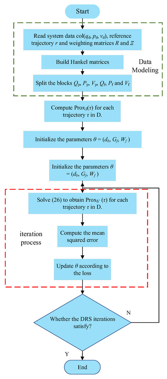
Figure 5.
Flow chart of voltage control solution based on DeePC algorithm.
5. Case Study
In this section, we introduce the modified IEEE 34-bus test system and present the simulation results. The primary objective is to verify the effectiveness and advantages of the proposed DeePC-based voltage controller.
5.1. Experimental Settings and Offline Data Collection
Figure 6 presents a schematic of the IEEE 34-bus test system, from which we extracted raw parameters and power dispatch information. Detailed information regarding the raw line impedance and shunt conductance is available in the literature [26]. The system’s base power and power/voltage ratings follow the specifications in [32]. The proposed voltage control strategy aims to regulate the bus voltage magnitude within the range of 0.95 to 1.05 p.u.
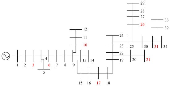
Figure 6.
The IEEE 34-bus test system. The red indexes indicate the buses with BESSs.
In this system, each bus is equipped with PV generation. We assume that the active and reactive power from PV generation, as well as the load at each bus, fluctuate slightly around their nominal values due to random noise. The upper and lower reactive power limits of the PV generation are adjusted based on the inverter rating, set to 9 kVA for active power output. Additionally, seven BESSs are strategically deployed at buses 3, 6, 10, 17, 21, 26, and 31.
For simulation purposes, substation bus voltages are fixed at 1 p.u. To ensure realistic conditions, we incorporate PV generation and load profiles at a 1 min resolution, as illustrated in Figure 7. Further details on the DeePC-based algorithm parameters can be found in Table 1, while Table 2 provides the parameters of the BESS.
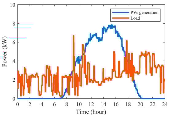
Figure 7.
Daily active power profiles of load and PV generation.

Table 1.
Parameters of the test system.
Table 2.
BESSs parameters.
The control parameters are carefully selected based on both physical insights and preliminary simulation studies. The prediction horizon Tf determines the time window over which future system behavior is optimized; a longer Tf improves long-term performance but increases computational burden. The historical horizon Tini captures recent system dynamics for state initialization in the prediction model, and is set to match the dominant time scales of load and generation variations.
Regularization weights λg, , , and penalize deviations from nominal control inputs and outputs in the initial trajectory, enhancing robustness against measurement noise and model inaccuracies. Specifically, a larger λg strengthens noise suppression but may slow down dynamic response. The control weighting matrices R and Ξ balance control effort against tracking performance, where higher values reduce actuator wear at the cost of slower voltage regulation. The penalty coefficient κ enforces constraint satisfaction in the optimization; a sufficiently large κ ensures feasibility but may amplify numerical sensitivity.
In Section 4, the proposed control method involves generating historical input–output trajectories offline using continuously stimulated input data. To enhance realism, process and measurement noise are incorporated into the simulation. The sampling period is set to 1 min, and the controller executes 1440 iterations with distinct datasets of length T to construct the Hankel matrix.
At the current sampling instant t, the voltage, the active power of the BESS, and the reactive power of the PV are predicted over the prediction range [t, t + Tf] using the collected historical trajectories and the initial trajectory of length Tini. The initial trajectory of the DeePC algorithm is updated at the next time instant t + ts by applying the first control input signal to the system at the current time instant. The whole process is repeated after ts time steps.
5.2. Simulation Results
In our simulations, we consider three different scenarios to demonstrate the effectiveness and advantage of our proposed data-driven approach. Our control objective is to maintain the voltage at each bus within the permissible range by controlling the power output of the controllable devices. And Figures 8–10 and 12 show the collective voltage profiles of all load buses over time, with each curve representing the voltage trajectory of one bus, illustrating the overall voltage distribution across the system.
Scenario 1—Basic Effectiveness Test: The disparity between PV generation and peak load demand heightens the vulnerability of distribution network to over-voltage conditions during midday and under-voltage in the evening. This effect is depicted in Figure 8, where voltage deviations are highlighted. In the absence of control strategy, the 34-bus test system undergoes significant voltage violations, resulting in bus voltages surpassing acceptable operational thresholds. Figure 9 presents the daily voltage profile achieved with the proposed data-driven control scheme. By analyzing the voltage control outcomes, it is evident that the proposed control strategy effectively maintains most bus voltages within the permissible range of 0.95 to 1.05 p.u.
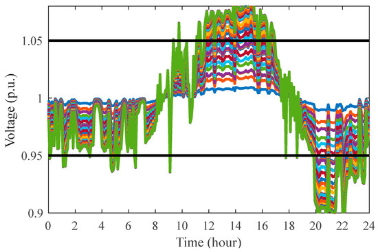
Figure 8.
Daily voltage profile across all load buses without control. (Each curve represents the voltage trajectory of one bus. The green curve with larger fluctuations is Bus 34; the blue curve with smaller fluctuations near 1.0 p.u. is Bus 1.).
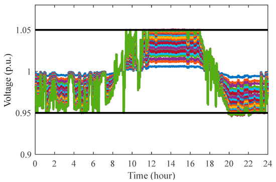
Figure 9.
Daily voltage profile across all load buses with the data-driven approach. (Each curve represents the voltage trajectory of one bus. The green curve with larger fluctuations is Bus 34; the blue curve with smaller fluctuations near 1.0 p.u. is Bus 1.).
Scenario 2—Comparison with the Model-based Method: To highlight the superiority of the proposed data-driven control methodology, its performance is evaluated in comparison to a model-based scheme, as referenced in (8). Unlike model-based strategies, which depend on specific system parameters, the data-driven approach circumvents the need for parameter identification. The comparative analysis, illustrated in Figure 9 and Figure 10, demonstrates that both control methods yield similar outcomes, validating the effectiveness of the proposed control strategy. Furthermore, Figure 11 provides a comparison of the RMS voltage averages between the two methods. Results indicate that the data-driven control approach is largely comparable to the model-based method in terms of control performance. Notably, the proposed DeePC voltage control method effectively addresses the voltage overrun issue, matching the traditional model-based strategy in its capacity to manage voltage levels. Moreover, the method enhances operational efficiency by regulating global voltage through local control, without requiring detailed knowledge of network topology or line parameters, thereby improving the economic operation of storage systems and enhancing overall practicality and performance.
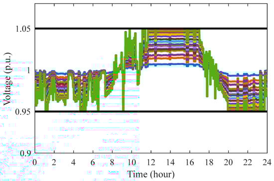
Figure 10.
Daily voltage profile across all load buses with the model-based approach. (Each curve represents the voltage trajectory of one bus. The green curve with larger fluctuations is Bus 34; the blue curve with smaller fluctuations near 1.0 p.u. is Bus 1.).
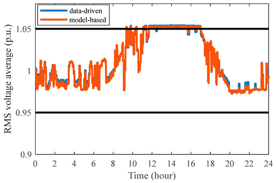
Figure 11.
Daily RMS voltage average with the model-based and data-driven approach.
Scenario 3—Robustness Test: To demonstrate the robustness of the proposed control strategy, the proposed data-driven controller is tested under changed system conditions. Particularly, the output power of PV generation at each bus was reduced by 5%, and the BESS was reallocated from buses 3, 6, 10, 17, 21, 26, and 31 to buses 4, 7, 11, 18, 22, 27, and 32. The resulting bus voltage profiles are presented in Figure 12. A comparison between Figure 9 and Figure 12 demonstrates that the proposed data-driven control method effectively mitigates voltage violation issues, maintaining control robustness despite changes in system parameters and network topology.
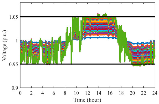
Figure 12.
Daily voltage profile across all load buses with the data-driven approach under changes in system parameters and topology. (Each curve represents the voltage trajectory of one bus. The green curve with larger fluctuations is Bus 34; the blue curve with smaller fluctuations near 1.0 p.u. is Bus 1.).
Figure 8, Figure 9, Figure 10 and Figure 12 illustrate the dynamic voltage responses across all buses. To further quantify performance differences, Table 3 summarizes the key voltage metrics, including Max Voltage Deviation, Average Voltage Deviation and Voltage Violation Duration Ratio under the three control strategies. It can be observed that both the model-based and data-driven approaches significantly reduce the maximum voltage deviation compared to no control and greatly decrease the voltage violation duration ratio. Notably, proposed data-driven control achieves performance on par with the model-based method, despite not relying on any explicit system model. For instance, the voltage violation duration ratio is reduced from approximately 18.1% in the no-control scenario to just 2.3% under the proposed data-driven control—very close to the 2.1% achieved by the model-based counterpart. This near-equivalent performance underscores the effectiveness of the proposed approach in learning accurate control policies directly from data, highlighting its potential as a practical and model-free solution for voltage regulation in active distribution networks.
Table 3.
Quantitative Comparison of Voltage Performance.
5.3. Parameter Sensitivity Analysis
To evaluate the robustness of the proposed controller to parameter variations, we conduct a sensitivity analysis on three key parameters: the regularization weight λg, the prediction horizon Tf, and the control effort weighting matrix R. Each parameter is varied across a representative range while keeping others fixed, and the closed-loop performance is assessed under the same test scenario as in Section 5.2.
Table 4 illustrates the impact of parameter variation on voltage regulation performance, measured by the root mean square error (RMSE) of node voltages, the total duration of voltage violations, and the number of energy storage system (ESS) charging/discharging cycles. As shown, increasing λg, from 1 to 10 reduces voltage RMSE by 18% due to improved noise filtering, but further increasing it to 100 leads to a 12% performance degradation due to sluggish response. A prediction horizon Tf of 30–60 s yields optimal trade-offs between performance and computational load; shorter horizons result in reactive control, while longer ones offer diminishing returns.
Table 4.
Performance comparison under different parameter settings.
Similarly, increasing R reduces ESS cycling by up to 30%, which is beneficial for battery longevity, but at the expense of a 20% increase in voltage RMSE. These results highlight the need for balanced parameter tuning in practical deployment. The current fixed-parameter design demonstrates acceptable robustness across tested ranges, though adaptive tuning could further enhance performance.
5.4. Comparative Performance Analysis
To further validate the effectiveness and practical advantages of the proposed data-driven voltage control strategy, this section presents a comprehensive study comparing its performance with representative methods, summarized in Table 5.
Table 5.
Comparison of Voltage Control Performance with Recent Studies.
While model-based MPC achieves good regulation accuracy, it relies on precise system models and suffers from high computational complexity. On the other hand, existing model-free reinforcement learning methods avoid modeling but require extensive training and exhibit limited generalization and real-time performance.
In contrast, the proposed method achieves a voltage violation duration ratio of 2.3% and a maximum deviation of 0.043 p.u., outperforming all listed learning-based approaches and closely matching the performance of model-based MPC—without requiring any system model or offline training. Moreover, its low online computational cost ensures high real-time feasibility. This demonstrates that the proposed strategy uniquely combines high accuracy, strong robustness, and ease of deployment, making it a superior choice for real-time voltage control in complex and uncertain distribution networks.
6. Conclusions and Future Works
In this paper, we present a novel DeePC-based control framework for bus voltage regulation in ADNs. The proposed framework leverages slack variables and regularization terms to effectively manage load uncertainties in net load conditions. Numerical case studies highlight the advantages of the data-driven voltage control approach, particularly in eliminating the need for precise physical modeling. Simulation results demonstrate that the data-driven controller reduces the voltage violation duration ratio from 18.1% (no control) to just 2.3%, with a maximum voltage deviation of 0.043 p.u.—performance that is comparable to model-based MPC (2.1%, 0.041 p.u.). Notably, the proposed data-driven control method effectively mitigates voltage violation issues, preserving control effectiveness despite variations in system parameters and network topology. Moreover, the reformulation using differentiable convex programming ensures low online computational burden, achieving high real-time feasibility.
Although the simulation validation in this work is based on the IEEE 34-bus system, the proposed scoring-function-based DeePC framework is inherently scalable and well-suited for larger distribution networks. The key lies in our reformulation of the original DeePC problem into a differentiable convex programming surrogate, which effectively mitigates the exponential growth of computational burden associated with large Hankel matrices in conventional DeePC. Specifically, the control policy is approximated by a fixed-dimensional parametric model trained offline, enabling real-time execution, for which the computational time is independent of the size of historical data. Furthermore, the architecture supports modular deployment; future extensions could leverage regional partitioning and coordinated local controllers to achieve distributed voltage regulation, thereby enhancing scalability. These features collectively ensure strong potential for application to larger systems, such as the IEEE 123-bus network or practical urban distribution grids.
For future work, we aim to investigate the integration of continuously stimulated large-scale input data and the application of the method to larger network topologies. Further research will also focus on validating the proposed solutions through practical implementation and testing on real power grids.
Author Contributions
Conceptualization, Y.L.; Methodology, Z.T.; Software, Q.L.; Validation, Y.L.; Formal analysis, Z.T. and Y.S.; Investigation, Y.Z.; Resources, Q.L.; Writing– original draft, Q.L. and Y.Z.; Writing– review and editing, Y.S. All authors have read and agreed to the published version of the manuscript.
Funding
This research received no external funding.
Data Availability Statement
The data presented in this study are available from the corresponding author upon reasonable request.
Conflicts of Interest
Author Yang Shi was employed by the company State Grid Ningbo Power Supply Company. The remaining authors declare that the research was conducted in the absence of any commercial or financial relationships that could be construed as a potential conflict of interest.
References
- Tonkoski, R.; Turcotte, D.; EL-Fouly, T.H.M. Impact of high pv penetration on voltage profiles in residential neighborhoods. IEEE Trans. Sustain. Energy 2012, 3, 518–527. [Google Scholar] [CrossRef]
- Ren, F.H.; Zhang, M.J.; Sutanto, D. A multi-agent solution to distribution system management by considering distributed generators. IEEE Trans. Power Syst. 2013, 28, 1442–1451. [Google Scholar] [CrossRef]
- Elkhatib, M.E.; El-Shatshat, R.; Salama, M.M.A. Novel coordinated voltage control for smart distribution networks with DG. IEEE Trans. Smart Grid 2011, 2, 598–605. [Google Scholar] [CrossRef]
- Von Appen, J.; Stetz, T.; Braun, M.; Schmiegel, A. Local voltage control strategies for pv storage systems in distribution grids. IEEE Trans. Smart Grid 2014, 5, 1002–1009. [Google Scholar] [CrossRef]
- Zeraati, M.; Golshan, M.E.H.; Guerrero, J. Distributed Control of Battery Energy Storage Systems for Voltage Regulation in Distribution Networks with High PV Penetration. IEEE Trans. Smart Grid 2017, 9, 3582–3593. [Google Scholar] [CrossRef]
- Wang, Y.; Tan, K.T.; Peng, X.Y.; So, P.L. Coordinated Control of Distributed Energy-Storage Systems for Voltage Regulation in Distribution Networks. IEEE Trans. Power Deliv. 2016, 31, 1132–1141. [Google Scholar] [CrossRef]
- Alam, M.J.E.; Muttaqi, K.M.; Sutanto, D. Mitigation of rooftop solar PV impacts and evening peak support by managing available capacity of distributed energy storage systems. IEEE Trans. Power Syst. 2013, 28, 3874–3884. [Google Scholar] [CrossRef]
- Kabir, M.N.; Mishra, Y.; Ledwich, G.; Dong, Z.Y.; Wong, K.P. Coordinated control of grid-connected photovoltaic reactive power and battery energy storage systems to improve the voltage profile of a residential distribution feeder. IEEE Trans. Ind. Inf. 2014, 10, 967–977. [Google Scholar] [CrossRef]
- Conti, S.; Greco, A.M.; Raiti, S. Local control of photovoltaic distributed generation for voltage regulation in LV distribution networks and simulation tools. Eur. Trans. Elect. Power 2009, 19, 798–813. [Google Scholar] [CrossRef]
- Hanif, A.; Choudhry, M. Dynamic voltage regulation and power export in a distribution system using distributed generation. J. Zhejiang Univ. Sci. A 2009, 10, 1523–1531. [Google Scholar] [CrossRef]
- Huo, Y.; Li, P.; Ji, H.; Yu, H.; Yan, J.; Wu, J.; Wang, C. Data-Driven Coordinated Voltage Control Method of Distribution Networks with High DG Penetration. IEEE Trans. Power Syst. 2023, 38, 1543–1557. [Google Scholar] [CrossRef]
- Hou, Z.; Jin, S. Data-driven model-free adaptive control for a class of MIMO nonlinear discrete-time system. IEEE Trans. Neural Netw. 2011, 22, 2173–2188. [Google Scholar]
- Al-Saffar, M.; Musilek, P. Reinforcement Learning-Based Distributed BESS Management for Mitigating Overvoltage Issues in Systems with High PV Penetration. IEEE Trans. Smart Grid 2020, 11, 2980–2994. [Google Scholar] [CrossRef]
- Li, Y.; Wu, J.; Pan, Y. Deep Reinforcement Learning for Online Scheduling of Photovoltaic Systems with Battery Energy Storage Systems. Intell. Converg. Netw. 2024, 5, 28–41. [Google Scholar] [CrossRef]
- Pei, Y.; Zhao, J.; Yao, Y.; Ding, F. Multi-Task Reinforcement Learning for Distribution System Voltage Control with Topology Changes. IEEE Trans. Smart Grid 2023, 14, 2481–2484. [Google Scholar] [CrossRef]
- Cao, D.; Zhao, J.; Hu, W.; Yu, N.; Ding, F.; Huang, Q.; Chen, Z. Deep Reinforcement Learning Enabled Physical-Model-Free Two-Timescale Voltage Control Method for Active Distribution Systems. IEEE Trans. Smart Grid 2022, 13, 149–165. [Google Scholar] [CrossRef]
- Baran, M.; Wu, F.F. Optimal sizing of capacitors placed on a radial distribution system. IEEE Trans. Power Deliv. 1989, 4, 735–743. [Google Scholar] [CrossRef]
- Markovsky, I.; Huang, L.; Dörfler, F. Data-driven control based on the behavioral approach: From theory to applications in power systems. IEEE Control Syst. 2023, 43, 28–68. [Google Scholar] [CrossRef]
- Fiedler, F.; Lucia, S. On the relationship between data-enabled predictive control and subspace predictive control. In Proceedings of the 2021 European Control Conference (ECC), Delft, The Netherlands, 29 June–2 July 2021; pp. 222–229. [Google Scholar]
- Huang, L.; Coulson, J.; Lygeros, J.; Dorfler, F. Data-Enabled Predictive Control for Grid-Connected Power Converters. In Proceedings of the 2019 IEEE 58th Conference on Decision and Control (CDC), Nice, France, 11–13 December 2019; pp. 8130–8135. [Google Scholar]
- Coulson, J.; Lygeros, J.; Dorfler, F. Distributionally Robust Chance Constrained Data-Enabled Predictive Control. IEEE Trans. Autom. Control 2022, 67, 3289–3304. [Google Scholar] [CrossRef]
- Yu, W.; Tang, Z.; Xiong, W. Distributed robust data-enabled predictive control based voltage control for networked microgrid system. Electr. Power Syst. Res. 2024, 231, 110360. [Google Scholar] [CrossRef]
- Kekatos, V.; Zhang, L.; Giannakis, G.B.; Baldick, R. Voltage Regulation Algorithms for Multiphase Power Distribution Grids. IEEE Trans. Power Syst. 2016, 31, 3913–3923. [Google Scholar] [CrossRef]
- Willems, J.C.; Rapisarda, P.; Markovsky, I.; De Moor, B.L.M. A note on persistency of excitation. Syst. Control Lett. 2005, 54, 325–329. [Google Scholar] [CrossRef]
- Lou, G.; Gu, W.; Lu, X.; Xu, Y.; Hong, H. Distributed Secondary Voltage Control in Islanded Microgrids with Consideration of Communication Network and Time Delays. IEEE Trans. Smart Grid 2020, 11, 3702–3715. [Google Scholar] [CrossRef]
- Su, X.; Masoum, M.A.S.; Wolfs, P.J. Optimal PV Inverter Reactive Power Control and Real Power Curtailment to Improve Performance of Unbalanced Four-Wire LV Distribution Networks. IEEE Trans. Sustain. Energy 2014, 5, 967–977. [Google Scholar] [CrossRef]
- Guo, C.; Wang, X.; Zheng, Y.; Zhang, F. Optimal energy management of multi-microgrids connected to distribution system based on deep reinforcement learning. Int. J. Electr. Power Energy Syst. 2021, 131, 107048. [Google Scholar] [CrossRef]
- Zhou, Y.; Lu, Y.; Li, Z.; Yan, J.; Mo, Y. Learning-Based Efficient Approximation of Data-Enabled Predictive Control. In Proceedings of the 2024 IEEE 63rd Conference on Decision and Control (CDC), Milan, Italy, 15–18 December 2024; pp. 322–327. [Google Scholar]
- Parikh, N.; Boyd, S. Proximal algorithms. Found. Trends Optim. 2014, 1, 127–239. [Google Scholar] [CrossRef]
- Monga, V.; Li, Y.; Eldar, Y.C. Algorithm unrolling: Interpretable, efficient deep learning for signal and image processing. IEEE Signal Process. Mag. 2021, 38, 18–44. [Google Scholar] [CrossRef]
- Eckstein, J.; Bertsekas, D.P. On the douglas—Rachford splitting method and the proximal point algorithm for maximal monotone operators. Math. Program. 1992, 55, 293–318. [Google Scholar] [CrossRef]
- Xiong, W.; Tang, Z.; Cui, X. Distributed data-driven voltage control for active distribution networks with changing grid topologies. Control Eng. Pract. 2024, 147, 105933. [Google Scholar] [CrossRef]
Disclaimer/Publisher’s Note: The statements, opinions and data contained in all publications are solely those of the individual author(s) and contributor(s) and not of MDPI and/or the editor(s). MDPI and/or the editor(s) disclaim responsibility for any injury to people or property resulting from any ideas, methods, instructions or products referred to in the content. |
© 2025 by the authors. Licensee MDPI, Basel, Switzerland. This article is an open access article distributed under the terms and conditions of the Creative Commons Attribution (CC BY) license (https://creativecommons.org/licenses/by/4.0/).