Self-Supervised Interpolation Method for Missing Shallow Subsurface Wavefield Data Based on SC-Net

Abstract

The inversion of shallow underground vibration fields primarily relies on signals collected by numerous sensors deployed on the surface. However, the accuracy of inversion is affected by the spatial distribution of these sensors. Therefore, under limited measurement points, signal reconstruction at unknown locations remains a critical challenge. To address this problem, we developed an SC-Net-based self-supervised interpolation method for missing wavefield data in shallow subsurface applications. This study utilizes incomplete seismic data acquired in real-world scenarios to train a neural network for seismic data interpolation, thereby expanding the sampled signals required for inversion. Since available seismic data samples are often scarce in practice, we adopt a hybrid training strategy combining simulated and real data. Specifically, a large number of numerically simulated samples are jointly trained with a limited set of real-world measurements. Furthermore, to enhance the robustness of network outputs, we integrate the Mean Teacher model framework and propose a self-supervised learning approach for missing data. Additionally, to enable the network to effectively capture long-range dependencies in both frequency and spatial domains of seismic data, we introduce a dual-branch feature fusion network that jointly models channel-wise and spatial relationships. Finally, in our actual field explosion experiments conducted at the test site, we demonstrated improved accuracy of our method through comparative analysis with several typical interpolation neural networks. Three ablation studies are also designed to demonstrate the effectiveness of the proposed approach.

1. Introduction

Shallow subsurface vibration field imaging is a critical technology for the accurate assessment of damage effects, as well as a foundational methodology for reconstructing both general underground vibration fields and those induced by explosions. In practical explosion monitoring scenarios, although deploying sensors across a small area reduces susceptibility to environmental and natural disturbances, limitations in budget often restrict the number of sensors that can be installed. This leads to spatially sparse signal acquisition and introduces gaps in the recorded data, thereby compromising the accuracy of field reconstruction. To address this issue, it is essential to perform interpolation at predetermined locations using signals acquired from the available sensor array.

Seismic data interpolation and reconstruction methods have undergone years of development, with scholars worldwide proposing various technical solutions. Among wave equation-based methods, Stolt [1] achieved data interpolation using the Born approximation, while Fomel [2] accomplished data recovery in the frequency domain through shot-receiver continuation. In low-rank constraint methods, Oropeza et al. [3] employed multichannel singular spectrum analysis, and Ma [4] applied low-rank matrix completion to 3D data reconstruction, capturing seismic data’s geometric features through low-rank components. Chen et al. [5] proposed a damped rank-reduction algorithm for 5D data interpolation. Prediction filtering methods assume seismic reflection signals exhibit linear event coherence. Porsani [6] improved the computational efficiency of Spitz’s method using a half-step prediction filter, while Naghizadeh et al. [7] designed a two-stage algorithm that first reconstructs low-frequency spectra via Fourier methods before extracting full-band prediction filters. Wu Geng et al. [8] addressed high-dimensional continuous missing data by proposing a high-order streaming prediction filtering interpolation method that enhances accuracy through additional constraints. Among various seismic data reconstruction algorithms, sparse transform-based methods hold significant importance. Traditional sparse transform reconstruction methods are based on compressed sensing theory, utilizing different sparse transforms to process data in sparse domains for reconstruction. However, in shallow subsurface seismic data acquisition, the extensive data gaps caused by constrained sensor deployment create high missing-rate scenarios. Under such conditions, conventional methods relying on data completeness and continuity assumptions prove inadequate for effective interpolation.

In recent years, deep learning (DL) has made remarkable progress in seismic data interpolation. Compared to traditional methods, DL techniques establish nonlinear mapping relationships between inputs and outputs, effectively integrating wave equation physics with data statistics to significantly improve reconstruction accuracy. For instance, S.N. et al. [9] previously proposed the application of autoencoders to address structural health monitoring problems in civil engineering. Wang et al. [10] employed dual generative adversarial networks to complete post-stack seismic data impedance inversion, while Zhou et al. [11] used DL to compensate for seismic signal absorption and attenuation. Wang et al. [12] achieved prestack viscoacoustic low-frequency extrapolation using an improved dense convolutional network. In well log reconstruction, Li Fenglin et al. [13] extracted features such as natural gamma and density through an encoder and established their mapping relationship with acoustic logs using a decoder to achieve high-precision reconstruction. Additionally, Liu Xia et al. [14] combined residual attention mechanisms to optimize seismic signal denoising performance, and Wan et al. [15] demonstrated that their proposed convolutional-deconvolutional network far surpassed traditional wavefield separation methods in suppressing reverse-time migration low-frequency noise. In seismic data interpolation and reconstruction, various DL methods have been applied. Jia et al. [16] combined sparse transforms with support vector regression to train models in sparse coefficient domains, while Siahkoohi et al. [17] developed a GAN-based reconstruction method. Wang et al. [18] implemented regular seismic data interpolation using residual networks, and Kaur et al. [19] proposed a cycle-consistent GAN algorithm. Xiong et al. [20] further optimized interpolation performance by combining improved deep residual networks with transfer learning strategies. Zheng Hao et al. [21] achieved intelligent seismic data interpolation using convolutional neural networks, and Wang et al. [22] completed irregular seismic data reconstruction through convolutional autoencoders.

Currently, most network models primarily focus on studying deep underground structures, which typically benefit from abundant real-world measurement data. However, this study addresses the challenge of shallow subsurface vibration inversion, where obtaining sufficient real data is difficult due to practical exploration cost constraints. To address this, we employ a joint training strategy combining simulated and real data, aiming to enhance the network’s interpolation capability for signals at unknown locations. Experiments reveal significant limitations in this mixed-data training approach: the training process exhibits unstable outputs, and the trained network demonstrates inconsistent performance across different noise environments, making it difficult to ensure stable interpolation quality. To overcome these issues, we introduce the Mean Teacher model framework and combine it with a self-supervised training strategy for missing data, effectively improving the model’s robustness and interpolation accuracy under data-scarce conditions.

Our main contributions are as follows:

(1)

We developed a deep interpolation network model named SC-Net, which incorporates our specifically designed spatial-channel feature fusion module to effectively integrate global and local features while capturing long-range dependencies. This approach proves particularly suitable for seismic data interpolation applications, as it reduces interpolation errors and generates reconstructed waveforms that more closely approximate the actual seismic waveforms. We conducted experimental tests under high missing-data conditions and achieved promising results.

(2)

Building upon the Mean Teacher model, we propose a plug-and-play training method for missing data. This approach enables training using only incomplete seismic data while enhancing network stability, making it adaptable to various complex real-world conditions.

(3)

To mitigate the challenge of insufficient real data for effective network training, we utilize a hybrid training approach combining simulated and real data. By jointly training the model with a large number of numerically simulated samples and a small set of real data samples, we enhance the model’s adaptability to shallow geological conditions, improve the generalization capability of the network model, and increase the accuracy of real seismic data interpolation. During our simulation experiments, we introduced Gaussian noise with varying amplitude percentages to the test data. The resulting outputs under different ablation scenarios demonstrate that our training framework can effectively enhance the network’s robustness to a certain extent.

2. Methods

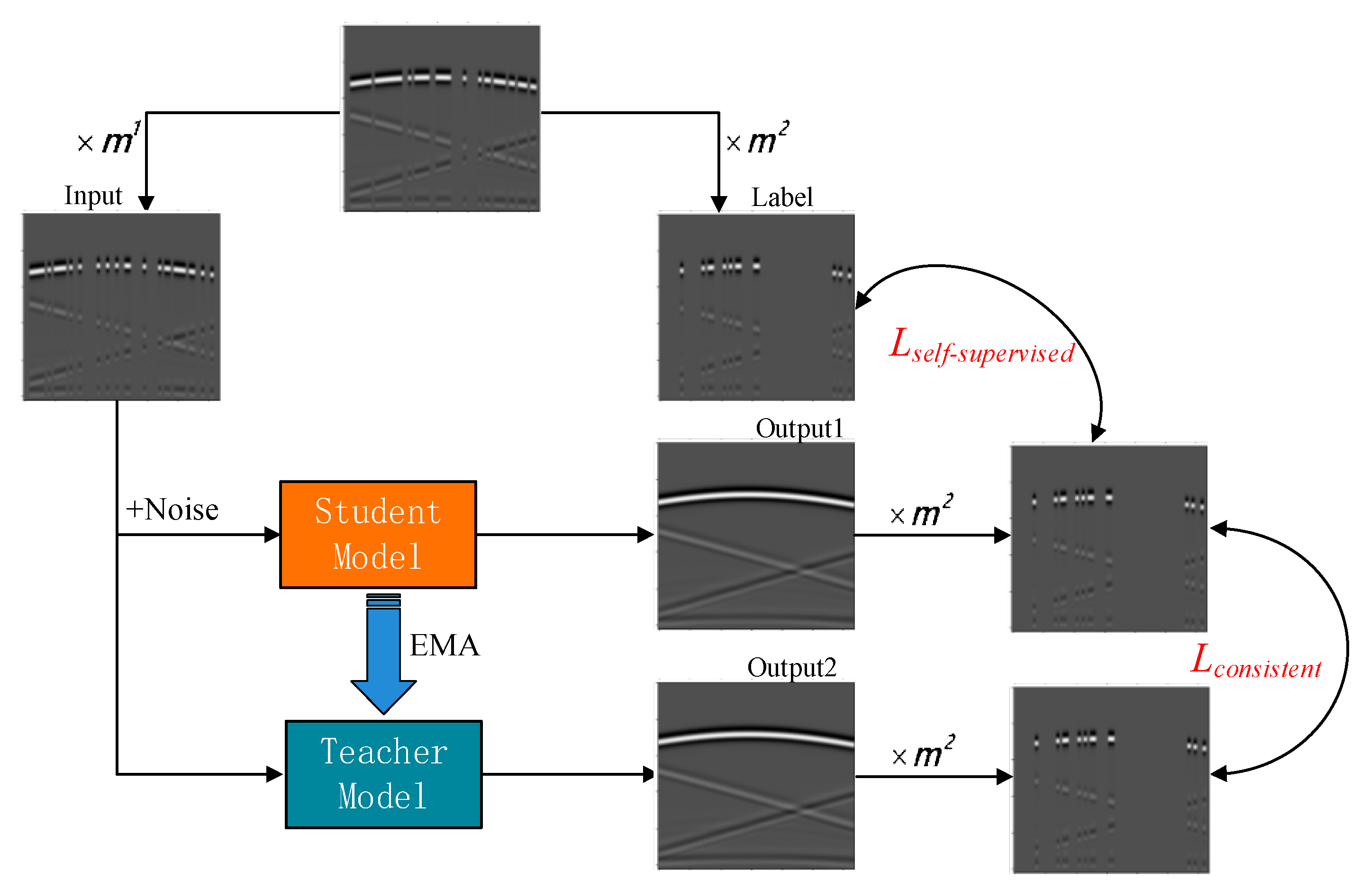
To achieve the objectives of subsequent experiments, we employ neural networks to perform interpolation on actual acquired signals while ensuring the network closely approximates the true seismic wave propagation patterns in subsurface formations. However, due to the limited availability of real data, we must supplement our training with substantial simulated data to effectively train our deep interpolation network. To address the scarcity of real data and enhance the training Dataset, while simultaneously improving the output robustness of the trained neural network, we have implemented an improved Mean Teacher Model. This approach introduces the concepts of teacher and student networks. The student model is trained through dual objectives: the reconstruction loss between its output and the original data labels, and the consistency loss with the pseudo-labels generated by the teacher model. Meanwhile, the teacher model’s parameters are gradually updated via an exponential moving average (EMA) mechanism, resulting in more stable interpolation outputs. Upon completion of training, the real incomplete data can be directly input into the trained teacher model to perform interpolation for the target measurement points. This approach ensures both data efficiency and result reliability in practical applications.

2.1. Spatial and Channel Feature Fusion Network (SC-Net)

We employ the U-net as the fundamental network architecture to achieve effective seismic data interpolation. As shown in Figure 1, it primarily consists of two components: an encoder and a decoder. The encoder is constructed with four down-sampling modules, while the decoder comprises three up-sampling modules, ultimately producing an output of the same size as the input through a Deconvolution layer. The specific structure is explained below:

2.1.1. Sampling Layer

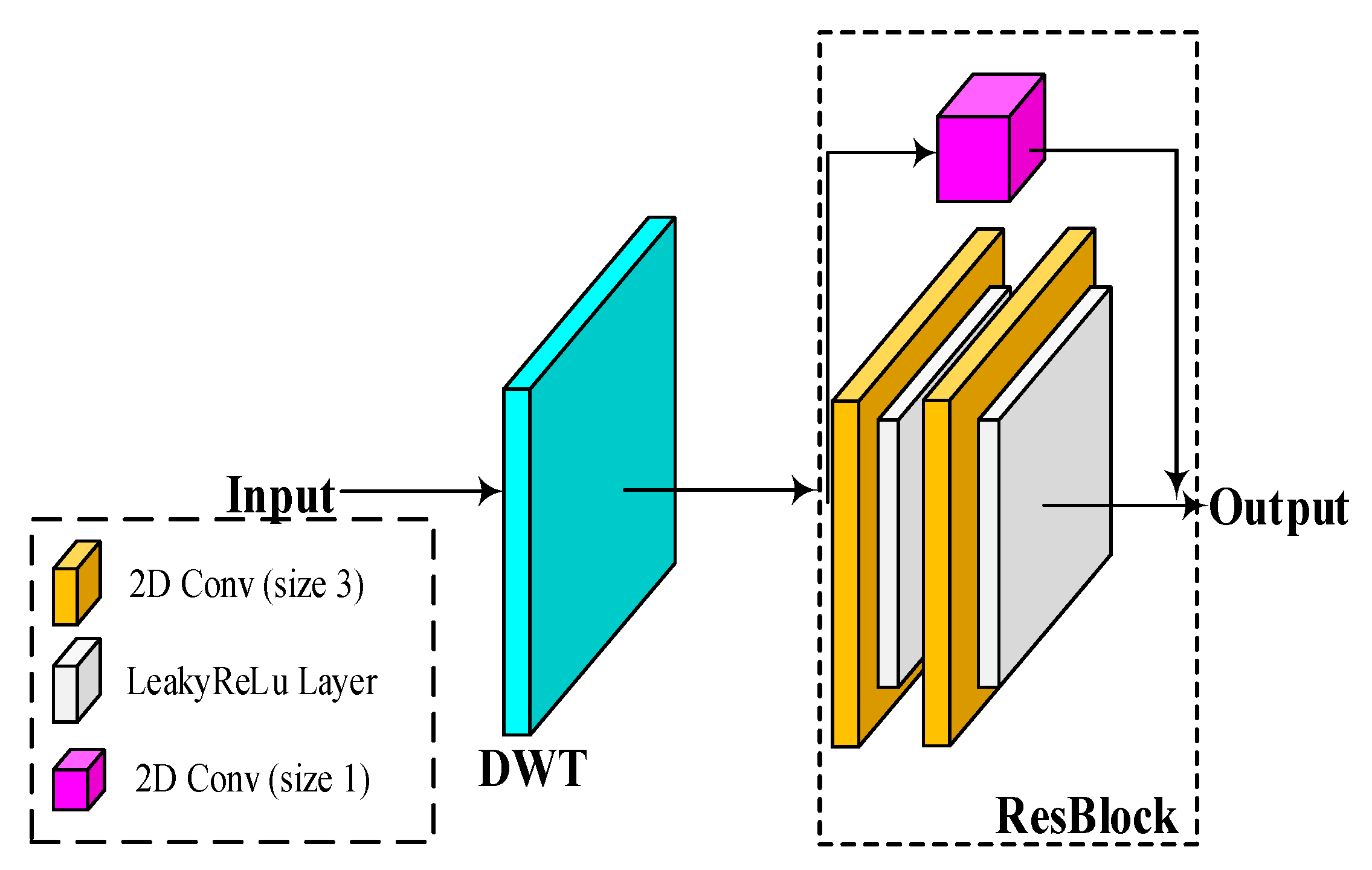
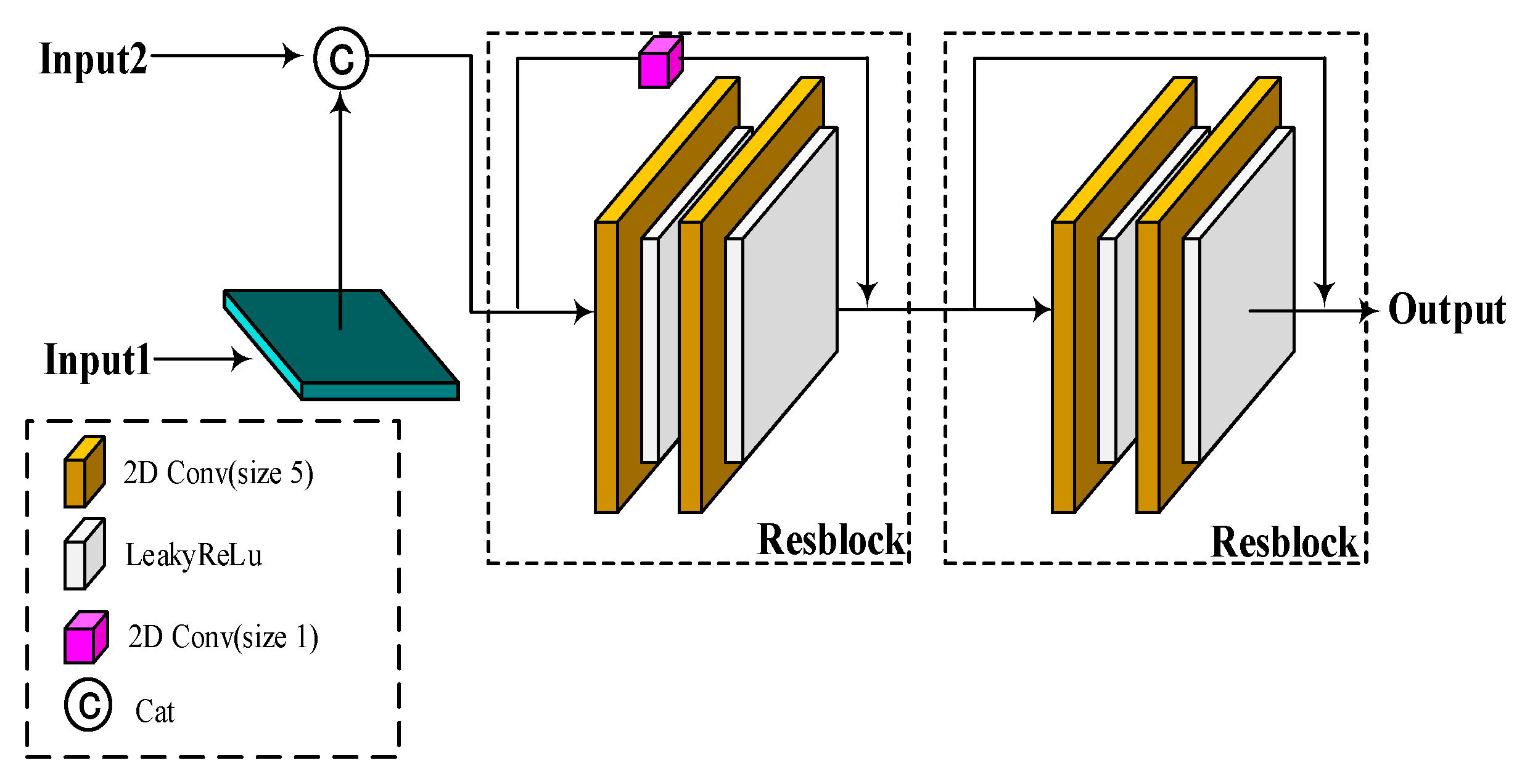
As illustrated in Figure 2, our designed down-sampling layer first processes the input through a wavelet down-sampling layer, which reduces data dimensions without information loss. Simultaneously, to prevent performance degradation caused by inefficient forward and backward information flow during training, we incorporate a residual block composed of “convolution, Leaky-ReLU layer, convolution, Leaky-ReLU layer”. As illustrated in Figure 3, the up-sampling layer is correspondingly configured with an inverse wavelet transform layer that mirrors the downsampling layer, along with the incorporation of two residual blocks. Where input2 represents the features to be fused from the upsampling module, while input1 denotes the features output by the previous module before this downsampling module. The wavelet transform is explained as follows:

• Wavelet down-sampling layer

Since the neural network takes incomplete seismic data as input, the encoder should strive to preserve all its essential features. To address the limitations of traditional downsampling methods—such as max pooling and average pooling—which tend to lose critical details like boundaries and textures during resolution reduction, we have adopted an alternative approach. Furthermore, these conventional methods are inherently irreversible: once pooling is applied for dimensionality reduction, the lost high-frequency information cannot be recovered from the pooled output. This characteristic is particularly detrimental to our seismic data interpolation task, which follows a “reduce dimensionality first, then reconstruct the original signal” workflow. Thus, we employ the Haar wavelet transform [23] as the downsampling layer. This transform decomposes the feature map into four components (one low-frequency and three high-frequency components). Although the spatial resolution is halved, all information is fully encoded into the channel dimension. This approach retains more edge or texture details in the missing seismic data, enabling the model to learn more representative features and thereby improving reconstruction performance. In the decoder, the inverse transform enhances interpolation accuracy.

A notable characteristic of the Discrete Wavelet Transform (DWT) is its adaptive spatial-frequency resolution capability: it achieves superior spatial resolution in high-frequency regions, allowing the detection of subtle faults in seismic data, while providing better frequency resolution in low-frequency regions, which helps mitigate the impact of high-frequency noise. Leveraging this advantage, the skip connections in our designed neural network incorporate a specially developed module (SC-FM) that suppresses noise-dominated high-frequency subband components. This design prevents the amplification of noise during the interpolation process and, when combined with the lossless reconstruction capability of the inverse transform, enables accurate seismic data recovery.

2.1.2. Spatial-Channel Feature Fusion Module (SC-FM)

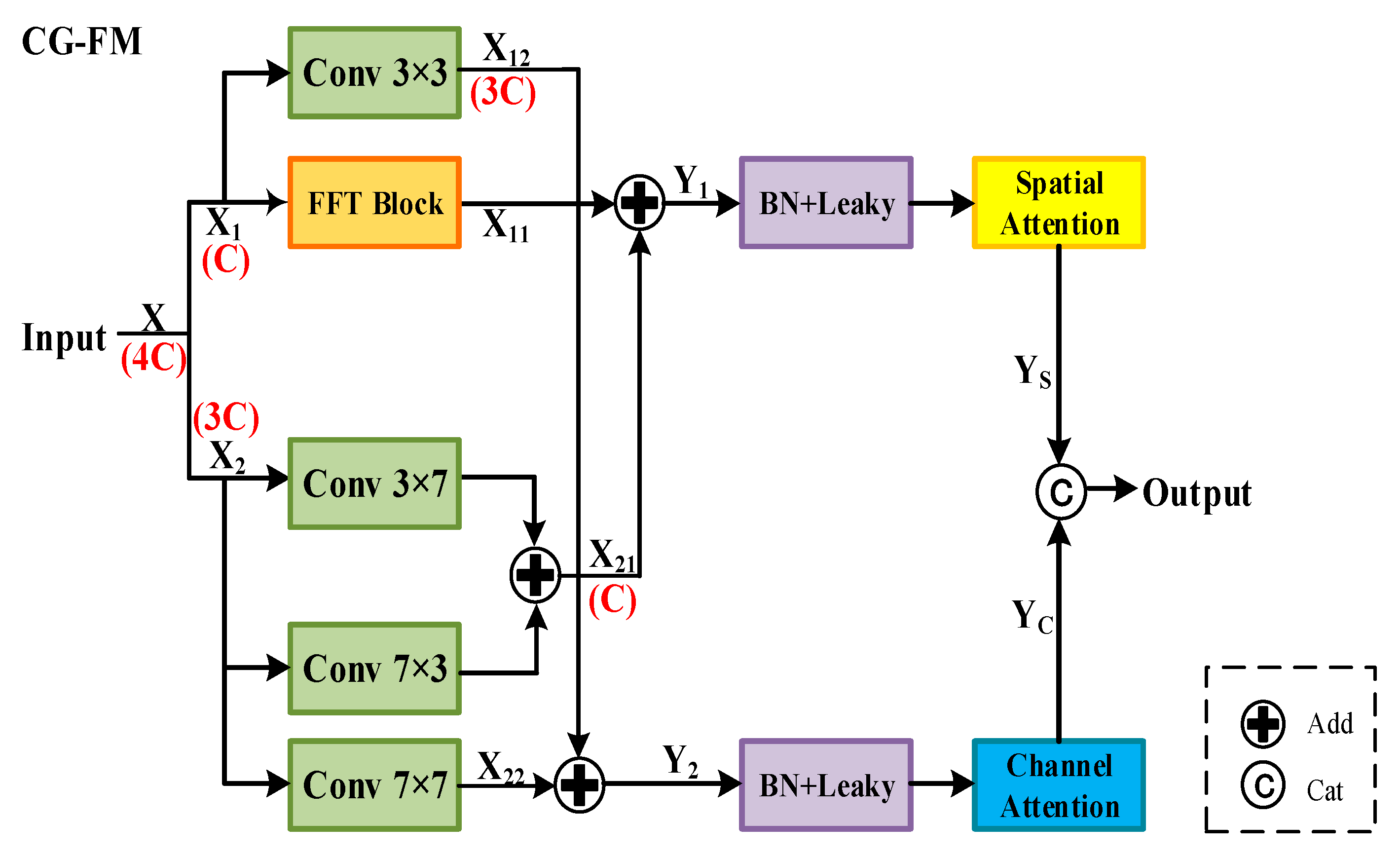
Multi-channel feature vectors are obtained via the wavelet transform. To suppress high-frequency subband components dominated by noise while preserving effective information in high-frequency subbands, we propose a Spatial-Channel Feature Fusion Module. As illustrated in Figure 4, this module mainly consists of two branches. Let the input feature be $\mathrm{X}\in {\mathbb{R}}^{4C\times H\times W}$, where $H\times W$ denotes the spatial resolution and 4C represents the number of channels. The first branch takes the low-frequency components from the first C channels as the input for global feature extraction, processing them through a 3 × 3 convolution and a Fourier transform module to obtain ${\mathrm{X}}_{12}$ and ${\mathrm{X}}_{11}$, respectively, which capture local and semi-global contextual information. The high-frequency detail features from the subsequent 3C channels serve as the input for local detail extraction, initially processed through 7 × 3 and 3 × 7 convolutions, followed by summation to produce ${\mathrm{X}}_{21}$. Thereby, it extracts local features from different spatial orientations and captures detailed spatial dimension information for each channel, such as edges and textures. Simultaneously, ${\mathrm{X}}_2$ is processed through a 7 × 7 convolution to generate ${\mathrm{X}}_{22}$, capturing medium-range local-to-semi-global features like wavefield correlations between multiple gathers, effectively balancing local details with regional continuity. As shown in Equation (1), ${\mathrm{Y}}_1$ and ${\mathrm{Y}}_2$ are, respectively, passed through a normalization layer and a Leaky ReLU layer. Subsequently, ${\mathrm{Y}}_1$ and ${\mathrm{Y}}_2$ go through a channel attention module and a spatial attention module, respectively. The spatial attention mechanism performs global feature enhancement on each feature map in ${\mathrm{Y}}_1$ to generate ${\mathrm{Y}}_{\mathrm{S}}$, while the channel attention mechanism enhances cross-channel relevant information in ${\mathrm{Y}}_2$ to obtain ${\mathrm{Y}}_{\mathrm{C}}$. The final output $\mathrm{Y}$ is the combined result of the set {${\mathrm{Y}}_{\mathrm{S}}$, ${\mathrm{Y}}_{\mathrm{C}}$}.

$$\left\{\begin{array}{c}{\mathrm{Y}}_1={\mathrm{X}}_{11}+{\mathrm{X}}_{21}\\ {\mathrm{Y}}_2={\mathrm{X}}_{12}+{\mathrm{X}}_{22}\end{array}\right.$$

(1)

2.

Spatial attention block

The Spatial attention primarily consists of three parallel Strip Attention (SSA) units. These employ simple convolutional branches to learn weights that aggregate contextual spatial information for each pixel from adjacent positions in the same row or column, achieving efficient information aggregation with low computational cost. Through horizontal and vertical strip attention operations [24], the module implicitly expands the network’s receptive field, enabling central pixels to perceive broader contextual regions and better capture long-range dependencies in the image.

As shown in Figure 5 and Figure 6, we implement three parallel SSAs with different strip lengths. In the encoder, we exclusively use horizontal strip attention units, while both horizontal and vertical strip attention units are employed in the decoder. For the horizontal strip processing, feature X first undergoes global average pooling (GAP), followed by 1 × 1 convolution and a Sigmoid function. The attention weight generation process can be expressed as:

$$\mathrm{A}=\mathrm{\sigma }\left(W_{1\times 1}\left(GAP\left(X\right)\right)\right)\in {\mathrm{R}}^K$$

(2)

where W_1×1 represents the 1 × 1 convolution, ‘$\mathrm{\sigma }$’ denotes the Sigmoid function, and K defines the integration length of the horizontal strip. We further improve efficiency by sharing A across the channel dimension. The refined features are then obtained through convolutional integration, with the computation for each output element following Equation (3). The final output features are obtained by summing the original input features with the processed features, and by combining the three SSA outputs of identical size.

$${\widehat{X}}_{c,h,w}={\displaystyle \sum _{k=0}^{K-1}{\mathrm{A}}_k{X}_{c,h,(w-[\frac{K}{2}]+k)}}$$

(3)

where ‘[·]’ represents rounding downwards. In seismic data interpolation, the encoder primarily serves to extract and compress features from the input seismic data, mapping high-dimensional data into a low-dimensional feature space. Given that seismic data typically exhibits vertical gaps, we exclusively employ horizontal strip attention mechanisms in the upsampling module to focus on lateral position characteristics and propagation patterns, such as the spatial continuity of geological formations. This approach enables concentrated attention on horizontal information, effectively extracts lateral features, while simultaneously reducing computational requirements and model complexity.

3.

Channel attention block

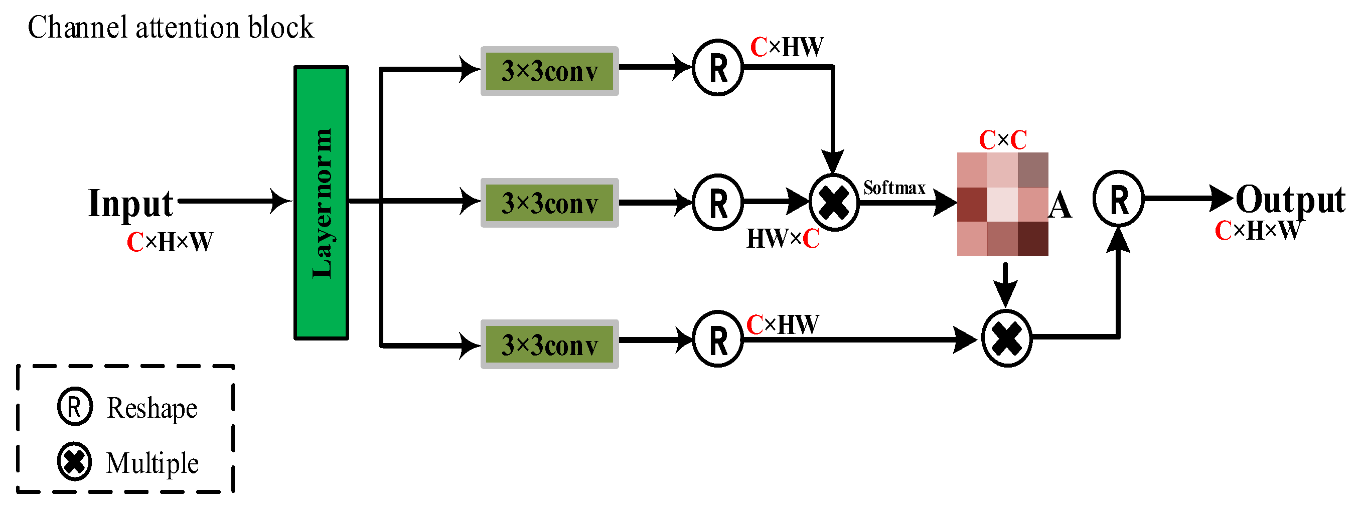
The channel attention block is illustrated in Figure 7. Specifically, tensors are obtained through layer normalization, followed by $3\times 3$ depthwise separable convolutions to generate projections for queries (Q), keys (K), and values (V). The query and key projections are reshaped so their dot product interaction produces a transposed attention map A of size C × C via Softmax. A is then multiplied with the value projection, and the result is processed through a 1 × 1 convolution before being added to the original features, yielding fused features of shape H × W × C. The T-LMM module enables the network to better capture and integrate important frequency components obtained from the Haar wavelet transform.

4.

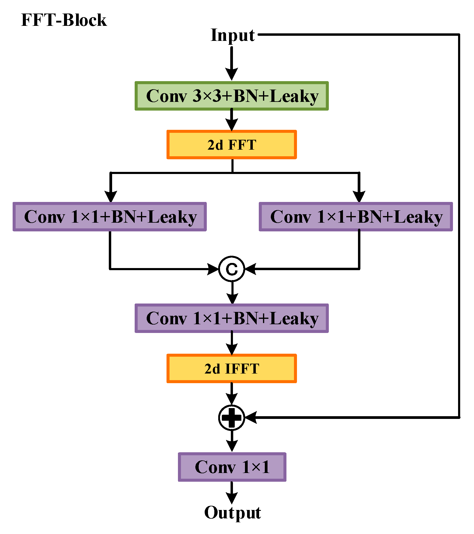
FFT block

We designed a Fourier transform block as illustrated in Figure 8. This module comprises two parallel branches, specifically employing Fourier components to extract global information from images, globally updating spectral data in the frequency domain, and subsequently converting it back to the spatial domain. Through channel-wise two-dimensional fast Fourier transform applied to input X, the complex frequency domain representation is expressed as:

$$\mathrm{X}\left[\mathrm{u},\mathrm{v}\right]={\displaystyle \sum _{n=0}^{N-1}{\displaystyle \sum _{m=0}^{M-1}\mathrm{x}\left[\mathrm{m},\mathrm{n}\right]\cdot }}{e}^{-j2\pi \left({\displaystyle \frac{um}{M}}+{\displaystyle \frac{vn}{N}}\right)}$$

(4)

where X[u,v] represents the complex coefficient corresponding to frequency indices (u,v) in the frequency domain, and x[m,n] denotes the pixel value at spatial position (m,n) of the image. Here, M indicates the image height while N represents the image width, with u and v corresponding to frequency indices ranging from 0 to M-1 and 0 to N-1, respectively. The imaginary and real components are initially processed as separate inputs through two parallel branches, each undergoing 1 × 1 convolution and Leaky ReLU activation. To achieve fusion of real and imaginary part information, the outputs are subsequently concatenated along the channel dimension, followed by another 1 × 1 convolutional layer with ReLU activation. Finally, the processed features are transformed back to the spatial domain via inverse Fourier transform.

To perform linear transformations along the channel dimension for each frequency coefficient while preserving the spatial dimensional structure of the frequency domain, this module employs 1 × 1 convolutions after the fast Fourier transform. This approach not only enables channel-wise interaction and optimization of frequency domain features, such as enhancing low-frequency global information channels and suppressing high-frequency noise channels, but also completely retains the global correlation characteristics of the frequency domain, which aligns well with our design objective of global modeling.

2.2. Self-Supervised Training Method for Missing Data

Let the incomplete data be denoted as $\mathbf{d}$, complete data as $\mathit{y}$, and sampling matrix as m. The objective of seismic data interpolation is to recover complete seismic data from the sampled incomplete data, which can be expressed as follows, where ‘$\circ$’ represents the Hadamard product (element-wise multiplication).

$$\mathbf{d}=\mathit{m}\circ \mathit{y}$$

(5)

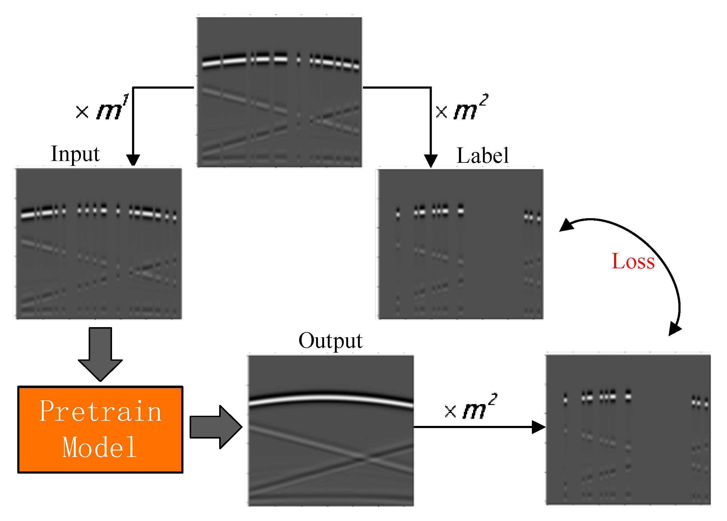
Based on the receptive field characteristics and weight sharing properties of convol ly partial data [25]. By ensuring each output element position has corresponding labeled elements through extensive training data, the network can reconstruct element values at corresponding positions during inference. This leads to the self-supervised training method for missing data shown in Figure 9.

The approach involves further masking the already incomplete data-one portion serves as network input while another portion acts as reconstruction labels. The network’s output at corresponding positions is then compared to establish the loss function.

Let ‘$o_i$’ represent an element in output sample ‘$o$’, and ‘$\theta$’ denote the network weight parameters. The loss function for a single sample is defined as:

$$Loss={\displaystyle \frac{1}{\left|{\mathsf{\Omega }}_m\right|}}\sum _{i\in {\mathsf{\Omega }}_m}{\left(o_i-{\mathrm{d}}_{\mathrm{i}}^{\mathrm{l}\mathrm{a}\mathrm{b}\mathrm{e}\mathrm{l}}\right)}^2$$

(6)

where $\left|{\mathsf{\Omega }}_m\right|$ represents the number of indices, making the loss function equivalent to:

$$Loss={\displaystyle \frac{1}{\left|{\mathsf{\Omega }}_m\right|}}\sum _{i\in {\mathsf{\Omega }}_m}{‖o-{\mathrm{d}}^{\mathrm{l}\mathrm{a}\mathrm{b}\mathrm{e}\mathrm{l}}‖}^2$$

(7)

During the training process, we combined simulated training data with real-world training data for model training and inference using this framework. However, the obtained results exhibited instability, specifically referring to inconsistent outputs when different noise patterns were introduced to the same input. This instability likely stems from inherent characteristic differences between simulated and real data. The simulated data, generated through forward modeling of elastic wave equations, features regular waveforms with extremely low noise levels, allowing precise prediction of wavefield propagation patterns. In contrast, the real data collected from explosive test sites contains waveform distortions due to sensor inaccuracies and environmental interference. Even after pre-processing with filtering techniques, the noise impact cannot be completely eliminated, leading to fundamental discrepancies in data characteristics that affect model performance consistency.

To address the challenges of effectively training neural networks under high missing rates and output instability caused by input noise, we incorporate the Mean Teacher Model [26] into this training framework. This semi-supervised learning approach employs a “teacher-student” dual-model structure, where the teacher model’s parameters are slowly updated via an exponential moving average (EMA) mechanism to produce more stable predictions. The student model simultaneously fits both the supervised signal (original seismic data) and the teacher model’s predictions, using consistency loss constraints to implicitly learn from unlabeled data (missing signals). This approach reduces dependence on large labeled datasets while enhancing model generalization through knowledge distillation from the teacher model-particularly valuable for label-scarce scenarios like seismic data interpolation.

In the specific context of shallow subsurface seismic data interpolation, this architectural advantage is particularly critical. As noted earlier, shallow seismic data suffers from two key limitations: scarce real-world labeled samples and unstable data distribution (due to environmental noise and differences between simulated and real data). The Mean Teacher Model’s semi-supervised learning paradigm reduces our reliance on large-scale labeled real seismic data— it can leverage unlabeled missing data (via consistency loss between student and teacher outputs) to implicitly learn the intrinsic wavefield propagation patterns. Meanwhile, the EMA-updated teacher network mitigates the output instability caused by the domain gap between simulated and real data, ensuring that the model maintains consistent interpolation performance even under high missing rates or varying noise levels [26].

As shown in Figure 10, both student and teacher models use identical SC-Net architectures with the same parameter counts. During the training of the student model, we deliberately introduce additional missing portions to the incomplete data-one segment serves as network input while another portion functions as training labels. Crucially, for any given sample, the missing components vary across different training epochs, achieved through dynamically generated random masks. To bridge the domain gap between simulated and real data during joint training, we pre-process the simulated data by injecting diverse noise patterns to better approximate real-world conditions, while maintaining a set of pristine simulated samples. For a single seismic signal, the specific formula is as follows.

$$S_{noisy}\left(t\right)=S_{sim}\left(t\right)+\gamma \cdot A_{sim}\cdot N\left(0,{\sigma }^2\right)$$

(8)

Here, $S_{noisy}\left(t\right)$ represents the simulated signal with added noise, $S_{sim}\left(t\right)$ denotes the single-channel sensor signal, $\gamma$ indicates the amplitude percentage coefficient (typically ranging from 0 to 1), and $A_{sim}$ represents the characteristic amplitude of the simulated data, which we express using the root mean square value. $N\left(0,{\sigma }^2\right)$ represents Gaussian noise with zero mean and ${\sigma }^2$ variance, while $\sigma$ is generally set to 1.

The model parameters are iteratively optimized via gradient descent algorithms with the explicit objective of loss function minimization. This dual strategy of randomized masking and noise augmentation significantly enhances the network’s robustness, improving both output consistency when handling slightly perturbed inputs and adaptability to shifting data distributions.

The parameters of the teacher model are derived from the exponential moving average (EMA) of the student model’s parameters. EMA is a smoothing technique for time-series data, where historical data points are assigned exponentially decreasing weights. This approach emphasizes the influence of recent data while diminishing the impact of older observations, thereby generating a stable and smoothed trend value. The formula is as follows:

$${\omega }_t=\beta \cdot {\omega }_t+\left(1-\beta \right)\cdot {\omega }_s$$

(9)

where ${\omega }_t$ represents teacher model parameters, ${\omega }_s$ represents student model parameters, and ‘$\beta$’ is the smoothing coefficient. This updating approach effectively filters out parameter oscillations caused by gradient fluctuations in the student model, thereby generating more stable parameters for the teacher model and preventing local optimum oscillations. This enables the model to better align with the global optimal trend of the data. Simultaneously, it enhances the model’s robustness and generalization capability, reducing sensitivity to minor input perturbations such as acquisition noise in seismic data. By mitigating overfitting, the method ensures consistent performance on test data, particularly with real-world data exhibiting distributional shifts, making it a crucial mechanism for addressing challenges like limited labeled data and input interference.

Since the teacher model’s parameters derive from the student model’s, only the student model’s loss function needs consideration for backpropagation updates. The total loss function combines: reconstruction loss between student model output and original data labels, and consistency loss with the teacher model’s pseudo-labels, incorporating $\left|{\mathsf{\Omega }}_m\right|$ as follows:

$$L_{total}=L_{sel\mathit{f-}supervised}+\lambda L_{consistent}$$

(10)

$$L_{self-supervised}={\displaystyle \frac{1}{\left|{\mathsf{\Omega }}_m\right|}}{{\displaystyle \sum _{i\in {\mathsf{\Omega }}_m}\left(o_i-d_i^{label}\right)}}^2$$

(11)

$$L_{consistent}={\displaystyle \frac{1}{\left|{\mathsf{\Omega }}_m\right|}}{{\displaystyle \sum _{i\in {\mathsf{\Omega }}_m}\left(o_i^S-o_i^T\right)}}^2$$

(12)

Here, L_{self-supervised} measures prediction differences between student model output and original data, while L_consistent calculates prediction discrepancies between student and teacher models across all signals (both missing and original portions). This consistency loss enforces agreement between student and teacher predictions, encouraging the model to learn intrinsic data structures-particularly for missing data interpolation.

Upon completion of training, the two-dimensional seismic data requiring interpolation is directly input into the teacher model, which generates an output of the same dimensions as the input. The missing portions in the original input are then replaced with the corresponding data from the output, thereby producing the complete interpolated seismic data. The mathematical expression is as follows, where d represents the incomplete data input to the network, m denotes the sampling matrix, and $o^S$ indicates the network output from the teacher model.

$$y=\left(\mathbf{1}-m\right)\circ o^S+\mathit{m}\circ \mathsf{d}$$

(13)

3. Results

3.1. Construction of Simulated Training Dataset

The performance of neural network training is highly dependent on the composition of the training dataset, as the quality of the data directly influences the interpolation capability of the resulting model. Our proposed SC-Net deep interpolation model processes seismic data as both input and output, leveraging the inherent connection between these data and the underlying geological structures. In the context of reconstructing shallow underground vibration signals, it is essential that the simulated training data accurately represent the complex propagation dynamics of shallow seismic wavefields—including reflections, transmissions, and other wave interactions. Given that the behavior of elastic waves is governed by fundamental wave propagation principles in subsurface media, and since soil structures and velocity models can be effectively represented through numerical methods, we utilize forward modeling based on the elastic wave equation. This approach allows us to generate synthetic data that faithfully captures the physical characteristics of typical shallow subsurface environments, thereby providing a realistic and physically consistent training foundation for the network. The real data in our study originates from seismic recordings of explosive sources, whose wavefield propagation intrinsically follows elastodynamic principles. The simulated data generated through this approach can accurately reproduce physical processes from actual acquisition mechanisms, including source radiation patterns and ground particle vibration directions. This ensures consistency in wavefield propagation mechanisms between simulated and real data. Such consistency effectively reduces the distributional discrepancy between simulated and real data, mitigating instability issues during mixed training while providing the network with a more reliable learning benchmark. The specific implementation is as follows:

Based on the stratigraphic information from the test site, we designed a shallow subsurface geological model comprising three layers: loess, paleosol, and calcareous gravel. To represent this model digitally, we constructed a 2D velocity matrix (60 m × 150 m) where the vertical dimension (z, 0–60 m) represents depth and the horizontal dimension (x, 0–150 m) represents lateral distance. Each matrix element corresponds to a 1 m × 1 m grid cell. The p-wave velocities were assigned as follows: 800 m/s for the upper layer (0–19 m depth), 1000 m/s for the intermediate layer (20–39 m), and 1500 m/s for the bottom layer (40–60 m).

The source excitation function for data simulation is configured as a Ricker wavelet with a dominant frequency of 60 Hz. Numerical simulation of p-waves is then performed using finite difference methods to solve the wave equation. The general formulation is expressed as follows:

$${\displaystyle \frac{{\partial }^{2}u}{\partial t^2}}=\upsilon {(x,z)}^2({\displaystyle \frac{{\partial }^{2}u}{\partial x^2}}+{\displaystyle \frac{{\partial }^{2}u}{\partial z^2}})+S(t)$$

(14)

First, the seismic sources were placed at depths ranging from 18 to 58 m with 2 m intervals, and at horizontal positions from x = 40 to 80 m with 1 m intervals. The sensor array was deployed at a depth of 1 m below the surface, spanning horizontally from 5 to 146 m with 1 m spacing. Using the elastic wave equation, the wavefield values at each sensor location were computed for all time steps. Concatenating these values chronologically yields the complete signal received by a single sensor. Each source point corresponds to a set of sensor signals, producing 451 signal groups in total. These signals are organized into gathers, and to facilitate network down/up-sampling, multiple complete gather samples are generated by sliding a $64\times 64$ pixel rectangular window across the gather plot with predefined horizontal and vertical strides.

3.2. Construction of Actual Training Dataset

The experimental area measures 150 m in length, 150 m in width, and 30 m in depth, with a grid resolution of 1 m to ensure sufficient spatial resolution for analyzing wave propagation characteristics. The coordinate system is defined with the positive x-axis oriented due east, positive y-axis due north, and positive z-axis upward from the reference plane at z = 0 (30 m below surface). Sensor locations were arranged at 5 m intervals along the y-axis and 1.5 m intervals along the x-axis. For each row (fixed y-coordinate), 45 sampling points were randomly selected for actual sensor deployment, ensuring each column contained at least one physical sensor to simulate missing data conditions. A spherical TNT charge with a 50 cm radius was detonated at the central point (60, 60, 30) using the center-initiation method.

The experiment employed a 50 cm-radius spherical TNT charge centered at (60, 60, 30) with central detonation. Thirty sets of sensor signals were organized into directional gather plots, with target interpolation points zeroed out and 5 traces per row retained as validation data. After processing per Section 3.1 methodology, the reconstructed results were input to the trained network. Output data were reassembled by position (averaging overlapping regions) and compared with held-out signals. This comparative validation approach effectively evaluates prediction accuracy.

Given that the network model takes image-formatted inputs, this study employs three image-based metrics to evaluate interpolation performance: the Structural Similarity Index Measure (SSIM), Peak Signal-to-Noise Ratio (PSNR), and Root Mean Square Error (RMSE).

3.3. Training and Results

We implemented the deep learning framework using PyTorch 2.6.0 with an RTX A6000 GPU, leveraging CUDA parallel computing architecture to accelerate training. The Adam optimizer was employed with an initial learning rate of 0.01 and a weight decay coefficient of 0.1 to mitigate overfitting. Training was conducted for 60 epochs with a batch size of 128. The ‘$\mathrm{\beta }$’ parameter in the mean teacher model is set to 0.9, and the consistency loss weight ‘$\lambda$’ is set to 1.0. To simulate realistic missing data conditions, we randomly removed approximately 40% of the data from each simulated sample. From these incomplete samples, an additional 20% was masked out at each epoch and used as network input, while the remaining 20% of missing traces served as ground truth labels for the reconstruction task.

3.3.1. Ablation Studies

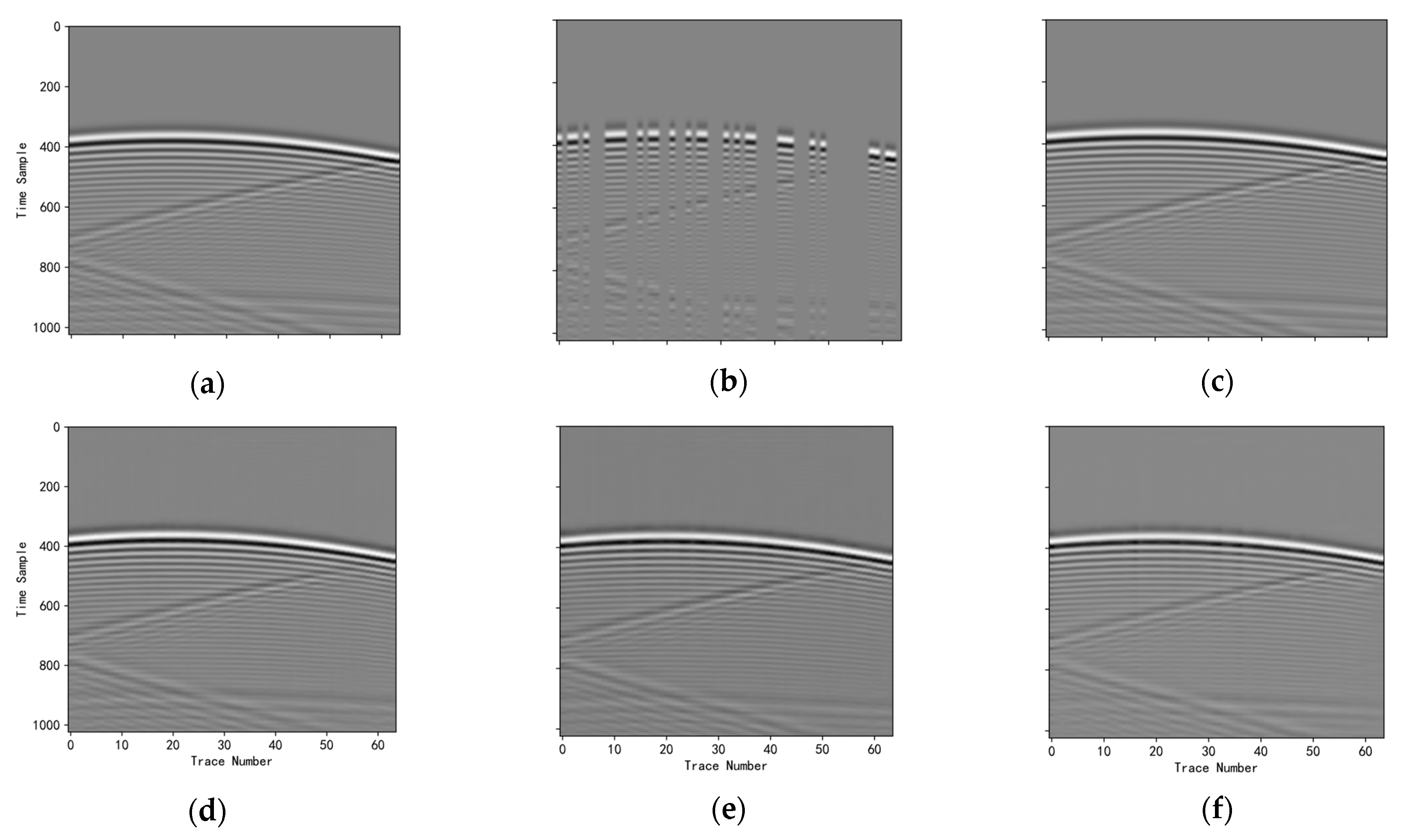
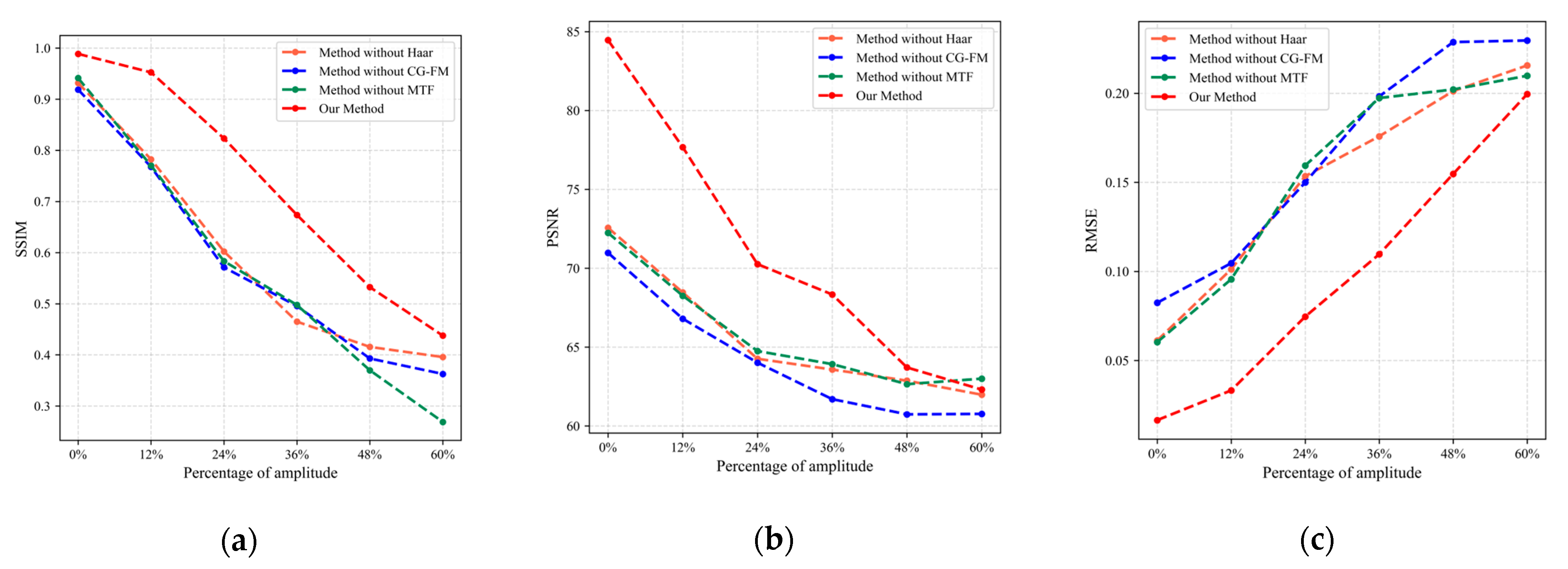
We conducted a series of ablation studies to evaluate the contributions of key components in our proposed framework. First, we replaced the wavelet-based down/upsampling layers with standard deconvolution and max-pooling operations to assess the advantage of wavelet transforms. Second, we removed the CG-FM entirely to validate its role in enhancing feature representation. Third, to evaluate our semi-supervised training strategy, we trained the network using only self-supervised learning on missing data without the Mean Teacher Framework (MTF). All models were tested under identical conditions using forward-modeled gather data from various source locations. The overall reconstruction performance is summarized in Figure 11. Additionally, we added different percentage amplitude noise to the same dataset as input and compared the three evaluation metrics in

Table 1. Add evaluation indicators for noise with different percentage amplitudes to each method.

Method	Metrics	0%	12%	24%	36%	48%	60%
Our Method	SSIM	0.9886	0.9524	0.8232	0.6736	0.5324	0.4376
	PSNR	84.4673	77.6743	70.2573	68.3341	63.7064	62.3021
	RMSE	0.0165	0.0332	0.0746	0.1096	0.1547	0.1995
Method-without Haar	SSIM	0.9316	0.7824	0.6021	0.4650	0.4156	0.3957
	PSNR	72.5634	68.4632	64.2573	63.5732	62.8673	61.9774
	RMSE	0.0612	0.1012	0.1534	0.1758	0.2012	0.2156
Method- without CG-FM	SSIM	0.9188	0.7676	0.5712	0.4954	0.3929	0.3627
	PSNR	70.9758	66.7961	64.0112	61.6954	60.7342	60.7594
	RMSE	0.0824	0.1046	0.1499	0.1982	0.2287	0.2296
Method-without MTF	SSIM	0.9412	0.7702	0.5832	0.4976	0.3698	0.2689
	PSNR	72.2414	68.2536	64.7463	63.9175	62.6476	62.9965
	RMSE	0.0603	0.0956	0.1594	0.1973	0.2021	0.2098

. The results demonstrate that our method exhibits better noise resistance, delivering superior performance compared to other methods even under significant noise conditions.

To provide a clear visual comparison of how different evaluation metrics vary under various noise conditions across ablation studies, the results are presented in Figure 12. It can be observed that our method consistently achieves the best overall performance across all metrics under different noise levels, even when Gaussian noise with 60% amplitude is added. The ablation variant without the CG-FM module demonstrates notably worse performance compared to the other two ablated configurations, underscoring the critical importance of the CG-FM module to our approach.

As illustrated in Figure 13, we provide a comparative analysis of the corresponding f-k spectra between the original and interpolated seismic gathers. The results clearly show that the spectra derived from our network’s output bear the closest resemblance to those of the original data, with better preservation of spectral continuity and wave-number characteristics. This high degree of alignment not only underscores the fidelity of our reconstruction but also reinforces the accuracy and effectiveness of the proposed method in maintaining the inherent physical properties of the wavefield. Such consistency in the frequency-wavenumber domain provides strong evidence that our approach successfully captures essential seismic structures while minimizing artifacts introduced during interpolation.

3.3.2. Network Effectiveness Comparison Experiments

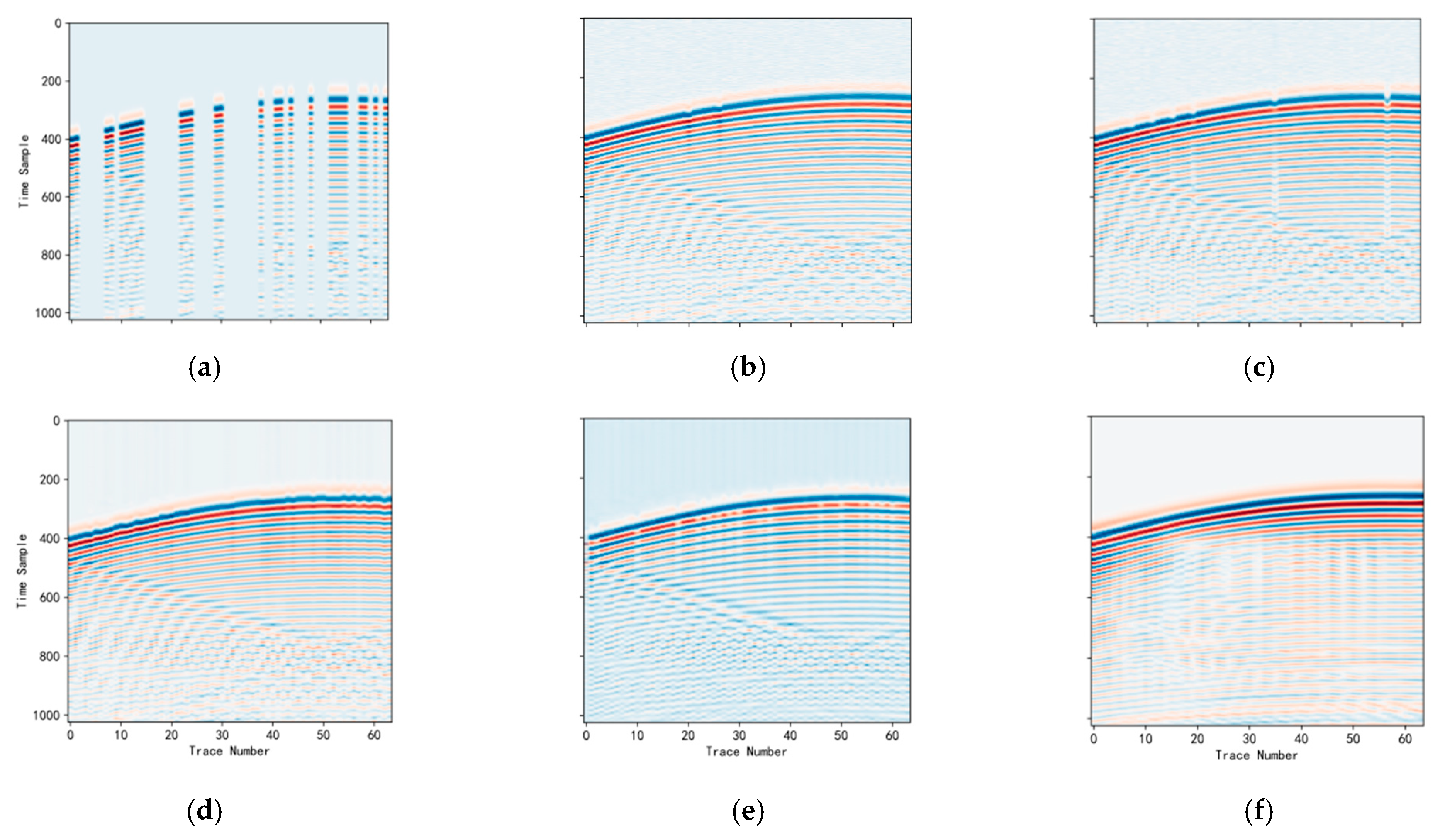
To validate the performance of our proposed network, we conducted comparative experiments against several established architectures: U-Net with residual connections (U-ResNet) [27], U-Net++ [28], Convolutional Autoencoders (CAE) [22], and MWCNN [29]. These models are canonical networks used for seismic data interpolation. All models were jointly trained on a combination of simulated and real datasets. Upon completion of training, each network was directly evaluated on real-world field data. Performance was assessed using the actual five traces per line excluded during training as the validation set. To ensure fair comparison and optimal performance across all models, the following hyperparameters were uniformly adopted: an initial learning rate of 0.001, a weight decay coefficient of 0.1, a batch size of 128, and training for 100 epochs.

The experimental results presented in Figure 14 demonstrate that our network produces reconstruction results that are not only smoother but also exhibit greater structural coherence compared to those generated by other methods. This visual advantage is further substantiated by the quantitative metrics provided in

Table 2. Comparison of five network metrics.

Method	SSIM	PSNR	RMSE
SC-Net	0.9212	76.5483	0.0332
MWCNN	0.8951	73.5850	0.0533
U-Net++	0.8679	71.3622	0.0588
U-Resnet	0.8566	71.1639	0.0642
CAE	0.6953	69.0816	0.0796

, which confirm that our predictions show a significantly stronger agreement with the held-out trace data. Meanwhile, the consistency between visual and numerical evaluations underscores the potential of our approach for practical applications where reliable data interpolation is critical.

4. Conclusions

To address the practical challenge of interpolating sparsely sampled seismic data, this study proposes an enhanced Mean Teacher training framework and introduces an efficient deep interpolation network named CG-Net. The methodology adopts a joint training strategy that utilizes both simulated and real-world data: large-scale training samples are first generated through forward modeling based on elastic wave equations, after which limited field seismic gathers containing the target interpolation traces are incorporated via a self-supervised learning approach with artificially masked data. Extensive comparative experiments confirm the superiority of the proposed network architecture and the effectiveness of the training strategy. This process produces interpolation results that more accurately reflect true wavefield propagation characteristics. The proposed “simulation-measurement” collaborative training paradigm offers a promising solution for data reconstruction in resource-limited settings.

References

1. Stolt, R.H. Seismic Data Mapping and Reconstruction. Geophysics 2002, 67, 890–908. [Google Scholar] [CrossRef]
2. Fomel, S. Seismic Reflection Data Interpolation with Differential Offset and Shot Continuation. Geophysics 2003, 68, 733–744. [Google Scholar] [CrossRef]
3. Oropeza, V.; Sacchi, M. Simultaneous Seismic Data Denoising and Reconstruction via Multichannel Singular Spectrum Analysis. Geophysics 2011, 76, V25–V32. [Google Scholar] [CrossRef]
4. Ma, J.W. Three-Dimensional Irregular Seismic Data Reconstruction via Low-Rank Matrix Completion. Geophysics 2013, 78, V181–V192. [Google Scholar] [CrossRef]
5. Chen, Y.K.; Zhang, D.; Huang, W.L.; Zu, S.; Jin, Z.; Chen, W. Damped Rank-Reduction Method for Simultaneous Denoising and Reconstruction of 5D Seismic Data. In Proceedings of the SEG Technical Program Expanded Abstracts, Dallas, TX, USA, 16–21 October 2016; Society of Exploration Geophysicists: Dallas, TX, USA, 2016; pp. 4075–4080. [Google Scholar]
6. Porsani, M. Seismic Trace Interpolation Using Half-Step Prediction Filters. Geophysics 1999, 64, 1461–1467. [Google Scholar] [CrossRef]
7. Naghizadeh, M.; Sacchi, M.D. Multistep Autoregressive Reconstruction of Seismic Records. Geophysics 2007, 72, V111–V118. [Google Scholar] [CrossRef]
8. Wu, G.; Liu, C.; Liu, D.; Liu, Y.; Zheng, Z. Seismic Data Interpolation Beyond Continuous Missing Data Using High-Order Streaming Prediction Filter. Chin. J. Geophys. 2023, 66, 1220–1231. [Google Scholar]
9. Pathirage, C.S.N.; Li, J.; Li, L.; Hao, H.; Liu, W.; Ni, P. Structural damage identification based on autoencoder neural networks and deep learning. Eng. Struct. 2018, 172, 13–28. [Google Scholar] [CrossRef]
10. Wang, Z.X.; Wang, S.D.; Zhou, C.; Cheng, W. Dual Wasserstein Generative Adversarial Network Condition: A Generative Adversarial Network-Based Acoustic Impedance Inversion Method. Geophysics 2022, 87, R401–R411. [Google Scholar] [CrossRef]
11. Zhou, C.; Wang, S.D.; Wang, Z.X.; Cheng, W. Absorption Attenuation Compensation Using an End-To-End Deep Neural Network. IEEE Trans. Geosci. Remote Sens. 2022, 60, 1–9. [Google Scholar] [CrossRef]
12. Wang, Z.Y.; Liu, G.C.; Du, J.; Li, C.; Qi, J. Low-Frequency Extrapolation of Prestack Viscoacoustic Seismic Data Based on Dense Convolutional Network. IEEE Trans. Geosci. Remote Sens. 2022, 60, 1–13. [Google Scholar] [CrossRef]
13. Li, F.; Liu, H.; Yang, X.; Zhao, M.; Yang, C.; Zhang, L. Reconstruction of Acoustic Curve Based on U-Net Neural Network. Period. Ocean. Univ. China 2023, 53, 86–92. [Google Scholar]
14. Liu, X.; Sun, Y. Seismic Signal Denoising Based on Convolutional Neural Network with Residual and Attention Mechanism. J. Jilin Univ. (Earth Sci. Ed.) 2023, 53, 609–621. [Google Scholar]
15. Wan, X.; Gong, X.; Cheng, Q.; Yu, M. Eliminating Low-Frequency Noise in Reverse-Time Migration Based on DeCNN. J. Jilin Univ. (Earth Sci. Ed.) 2023, 53, 1593–1601. [Google Scholar]
16. Jia, Y.N.; Ma, J.W. What Can Machine Learning Do for Seismic Data Processing? An Interpolation Application. Geophysics 2017, 82, V163–V177. [Google Scholar] [CrossRef]
17. Siahkoohi, A.; Kumar, R.; Herrmann, F. Seismic Data Reconstruction with Generative Adversarial Networks. In Proceedings of the 80th EAGE Conference and Exhibition, Copenhagen, Denmark, 11–14 June 2018; European Association of Geoscientists and Engineers: Copenhagen, Denmark, 2018; pp. 1–5. [Google Scholar]
18. Wang, B.F.; Zhang, N.; Lu, W.K.; Wang, J. Deep-Learning-Based Seismic Data Interpolation: A Preliminary Result. Geophysics 2019, 84, V11–V20. [Google Scholar] [CrossRef]
19. Kaur, H.; Pham, N.; Fomel, S. Seismic Data Interpolation using CycleGAN. In Proceedings of the SEG Technical Program Expanded Abstracts, San Antonio, TX, USA, 19–20 September 2019; Society of Exploration Geophysicists: San Antonio, TX, USA, 2019; pp. 2202–2206. [Google Scholar]
20. Xiong, Y.; Cheng, J. Efficient Seismic Data Interpolation using Deep Convolutional Networks and Transfer Learning. In Proceedings of the 81st EAGE Conference and Exhibition, London, UK, 3–6 June 2019; European Association of Geoscientists and Engineers: London, UK, 2019; pp. 1–5. [Google Scholar]
21. Zheng, H.; Zhang, B. Intelligent Seismic Data Interpolation via Convolutional Neural Network. Prog. Geophys. 2020, 35, 721–727. [Google Scholar]
22. Wang, Y.Y.; Wang, B.F.; Tu, N.; Geng, J. Seismic Trace Interpolation for Irregularly Spatial Sampled Data Using Convolutional Auto-Encoder. Geophysics 2020, 85, V119–V130. [Google Scholar] [CrossRef]
23. Xu, G.; Liao, W.; Zhang, X.; Li, C.; He, X.; Wu, X. Haar wavelet downsampling: A simple but effective downsampling module for semantic segmentation. Pattern Recognit. 2023, 143, 109819. [Google Scholar] [CrossRef]
24. Cui, Y.; Alois, K. Dual-domain strip attention for image restoration. Neural Netw. 2024, 171, 429–439. [Google Scholar] [CrossRef] [PubMed]
25. Fang, W.; Fu, L.; Wu, M.; Yue, J.; Li, H. Irregularly sampled seismic data interpolation with self-supervised learning. Geophysics 2023, 88, V175–V185. [Google Scholar] [CrossRef]
26. Tarvainen, A.; Harri, V. Mean teachers are better role models: Weight-averaged consistency targets improve semi-supervised deep learning results. In Advances in Neural Information Processing Systems; MIT Press: Cambridge, MA, USA, 2017; Available online: https://dl.acm.org/doi/10.5555/3294771.3294885 (accessed on 1 October 2025).
27. Hwang, S.; Jeon, S.; Ma, Y.S. Byun, H. WeatherGAN: Unsupervised multi-weather image-to-image translation via single content-preserving UResNet generator. Multimedia Tools Appl. 2022, 81, 40269–40288. [Google Scholar] [CrossRef]
28. Zhou, Z.; Siddiquee, M.M.R.; Tajbakhsh, N.; Liang, J. Unet++: A nested u-net architecture for medical image segmentation. In Proceedings of the International Workshop on Deep Learning in Medical Image Analysis, Granada, Spain, 20 September 2018; Springer International Publishing: Cham, Switzerland, 2018. [Google Scholar]
29. Liu, P.; Zhang, H.; Zhang, K.; Lin, L.; Zuo, W. Multi-level wavelet-CNN for image restoration. In Proceedings of the IEEE Conference on Computer Vision and Pattern Recognition Workshops, Salt Lake City, UT, USA, 18–23 June 2018; pp. 773–782. [Google Scholar]
Figure 1. SC-Net Overall Framework.
Electronics 14 04185 g001
Figure 2. Down-sampling module architecture.
Electronics 14 04185 g002
Figure 3. Up-sampling module architecture.
Electronics 14 04185 g003
Figure 4. SC-FM module structure.
Electronics 14 04185 g004
Figure 5. Spatial attention block structure.
Electronics 14 04185 g005
Figure 6. SSA module structure.
Electronics 14 04185 g006
Figure 7. Channel attention block structure.
Electronics 14 04185 g007
Figure 8. FFT Block structure.
Electronics 14 04185 g008
Figure 9. Self-supervised training framework.
Electronics 14 04185 g009
Figure 10. Improved self-supervised Mean-Teacher-Model for missing data.
Electronics 14 04185 g010
Figure 11. Experimental results: (a) Complete data; (b) Missing 70% of data; (c) The result obtained by our method; (d) Result obtained from Method 1; (e) Result obtained from Method 2; (f) Result obtained from Method 3.
Electronics 14 04185 g011
Figure 12. Experimental results: (a) Structural Similarity Index Measure; (b) Peak Signal-to-Noise Ratio; (c) Root Mean Square Error.
Electronics 14 04185 g012
Figure 13. The f-k spectrum of the experimental results: (a) Complete data; (be) represent the above four training modalities in turn.
Electronics 14 04185 g013
Figure 14. Actual experimental results: (a) Missing data; (b) Result from SC-Net; (c) Result from MWCNN; (d) Result from U-Net++; (e) Result from U-Resnet; (f) Result from CAE.
Electronics 14 04185 g014