A Lightweight, Explainable Spam Detection System with Rüppell’s Fox Optimizer for the Social Media Network X

Abstract

Effective spam detection systems are essential in online social media networks (OSNs) and cybersecurity, and they directly influence the quality of decision-making pertaining to security. With today’s digital communications, unsolicited spam degrades user experiences and threatens platform security. Machine learning-based spam detection systems offer an automated defense. Despite their effectiveness, such methods are frequently hindered by the “black box” problem, an interpretability deficiency that constrains their deployment in security applications, which, in order to comprehend the rationale of classification processes, is crucial for efficient threat evaluation and response strategies. However, their effectiveness hinges on selecting an optimal feature subset. To address these issues, we propose a lightweight, explainable spam detection model that integrates a nature-inspired optimizer. The approach employs clean data with data preprocessing and feature selection using a swarm-based, nature-inspired meta-heuristic Rüppell’s Fox Optimization (RFO) algorithm. To the best of our knowledge, this is the first time the algorithm has been adapted to the field of cybersecurity. The resulting minimal feature set is used to train a supervised classifier that achieves high detection rates and accuracy with respect to spam accounts. For the interpretation of model predictions, Shapley values are computed and illustrated through swarm and summary charts. The proposed system was empirically assessed using two datasets, achieving accuracies of 99.10%, 98.77%, 96.57%, and 92.24% on Dataset 1 using RFO with DT, KNN, AdaBoost, and LR and 98.94%, 98.67%, 95.04%, and 94.52% on Dataset 2, respectively. The results validate the efficacy of the suggested approach, providing an accurate and understandable model for spam account identification. This study represents notable progress in the field, offering a thorough and dependable resolution for spam account detection issues.

1. Introduction

In the modern era, online social networks (OSNs) have emerged, with the main information source X, previously named “Twitter”, being one of the most prominent and extensively utilized OSN platforms. Consequently, it contributes significantly to online discussions and links millions of users. Nonetheless, their significant impact renders it an appealing target for nefarious individuals aiming to control and sway public perspectives and decision processes [1,2]. X is a frequent target due to its free structure and growing user demographic. The X platform considers spam an essential issue and employs multiple spam filters to safeguard users [3,4,5,6,7,8]. Spam X accounts utilize new techniques and behaviors. Consequently, the utilization of new adaptive and robust technologies for detecting spam X accounts has become imperative. The use of artificial intelligence (AI) with machine learning (ML) presents a viable solution. Models using ML can learn from real-world datasets by employing algorithms such as ensemble learning, DT, KNN, and LR and can be used to successfully differentiate spam from non-spam accounts. Such techniques provide a more powerful and dynamic method, as they are able to adjust to modern spamming strategies [9,10].

A major challenge in implementing ML models is the “black box” problem. ML models are often black boxes, making their predictions difficult to understand—especially in cybersecurity activities such as spam detection, where the predictions from these models can be complex and challenging for cybersecurity specialists to interpret. Consequently, architecture must be developed to clarify the predictions of ML spam detection systems. The solution to some of these problems has emerged in the form of the XAI approach [11]. This approach seeks to address gaps in elucidating predictions generated by ML models within the realm of cybersecurity applications [12]. XAI clarifies the black box system by interpreting its operations and predictions.

This study highlights the needed measures by offering an innovative approach for developing an ML-driven spam detection system that is lightweight, where the trained model uses the optimal subset of features. This facilitates a reduction in computation resources for spam detection. This study provides a feature selection method that utilizes a swarm-based, nature-inspired meta-heuristic method: RFO [13]. Moreover, the proposed system is both learned and evaluated via ML methods. The predicted outcome generated via a learned ML-driven spam detection model is elucidated through employing the SHapley Additive exPlanations (SHAP) values [14]. This study’s primary contributions are delineated as follows:

• An innovative XAI-powered machine learning model that significantly improves classification accuracy in X spam account detection is proposed.
• A swarm-based, nature-inspired meta-heuristic method—called Rüppell’s Fox Optimizer (RFO) algorithm—for feature selection is proposed, which—to the best of our knowledge—is applied to cybersecurity and lightweight system loads for the first time.
• The proposed solution is experimentally evaluated using a real-world X dataset. The developed model significantly improves performance metrics such as confusion matrix, precision, recall, accuracy, F1 score, and the area-under-the-curve (AUC) value.
• The prediction made by the ML-driven spam detection model is interpreted by computing the Shapley values through the SHAP methodology.

The remainder of this study is structured as follows: In Section 2, the background of XAI and ML algorithms is outlined. Section 3 presents a summary of experiments employing artificial intelligence methodologies, including ML, DL, and FL, for X social network spam detection, along with their outcomes. Section 4 clarifies the methods and materials employed for X social network spam identification, as well as the performance metrics utilized to assess the efficacy of the applied methodologies. Section 5 presents the outcomes of the experiments for all models and discusses their findings. The final section presents overarching assessments of the outcomes.

2. Background

This section provides a detailed overview of the key concepts and classification algorithms underlying the proposed spam detection system. Furthermore, explainable artificial intelligence (XAI) and SHAP methods—which are employed to interpret the model’s decision-making processes—are proposed.

2.1. Explainable Artificial Intelligence

The imperative for understanding the procedures inherent in AI models’ decision-making has resulted in the emergence of XAI. The principal aim of this approach is to transparently reveal what a model predicts, why it makes those predictions, and how a model makes predictions, in addition to the rationale behind those predictions [15] and the methodology employed in reaching the conclusions (as shown in Figure 1).

Making the internal mechanisms of black box models understandable is critical with respect to reliability, ethical compliance, and debugging. In particular, in highly interactive applications such as social network platform spam detection, the explainability of decisions, as shown in Figure 2, is vital for both user satisfaction and compliance with legal regulations [16].

SHAP (SHapley Additive exPlanations) produces model explanations at both global (entire dataset) and local (individual instance) levels using Shapley values derived from cooperative game theory, as shown in Figure 3. The contribution of each feature to the decision process is calculated by averaging the marginal effects over all feature combinations [17,18].

2.2. Machine Learning Algorithms

The comparison analysis is a crucial element of this study, providing an overall structure for evaluating the effectiveness of the proposed system.

A decision tree (DT) is a supervised machine-learning algorithm that is widely used in classification and regression problems. The model divides the data into subsets in successive internal nodes starting from the root node and the final class; in other cases, the numerical output is produced in leaf nodes [19]. Data splitting decisions are usually based on measures such as entropy, information gain, or the Gini index. The aim is to reduce the irregularity of the target variable as much as possible within each split [19]. Decision trees provide understandable models on their own thanks to their interpretable structures; they also play a critical role as the base learner in ensemble techniques such as AdaBoost. These ensemble models increase accuracy by balancing the high variance of individual trees. In text classification applications, such as spam detection in social networks, decision trees are preferred due to both their fast prediction times and explainability advantages; they provide high accuracy when used alone or in an ensemble [20].

K-nearest neighbors, abbreviated as KNN, represent a non-parametric, lazy learning technique utilized for regression and classification tasks. Instead of developing a definitive model, all calculations take place during the prediction phase [21]. The core idea entails designating a query instance with the label (or value) that is most prevalent over its ќ nearest neighbors within the learning dataset [22]. KNN’s straightforward implementation and its independence from any assumptions about the underlying data distribution have rendered it a widely adopted method in numerous domains, including spam social network detection [23].

Logistic regression (LR) represents a fundamental ML technique employed in classification applications. It creates a model of the probability that an input falls into a specific class. The objective of LR is to develop a model capable of making a classification decision using the sigmoid function [24]. The high interpretability and computationally efficient nature of LR allow it to stand out in both explanatory analysis and practical applications such as spam detection [25]. For example, models that predict social media interactions based on graph and content features can clearly reveal the effects of variables thanks to the understandable structure of linear regression [26].

Ensemble learning in the ML field seeks to improve overall performance and generalizability by integrating the predictions of various classifiers or regression models. In this approach, various weak learners are aggregated to counterbalance their individual faults, resulting in a more solid composite model. Three principal ensemble learning strategies are defined: bagging, boosting, and stacking. In addition, model and error diversity play a key role in these strategies. Thus, ensemble approaches alleviate overfitting inclinations and the accuracy deficiencies observed in individual models, bringing about enhanced task performance and high precision, such as in social network spam identification [27,28].

This study employs the boosting algorithm AdaBoost. AdaBoost is an iterative improvement technique wherein weak learners are taught consecutively, with increased focus on previously misclassified instances at each stage. AdaBoost constructs its final decision through weighted voting for each weak learner, utilizing decision stumps as base learners. This system allows basic classifiers to collaboratively attain elevated accuracy. Moreover, AdaBoost’s nonparametric characteristics and its inherent technique for mitigating overfitting enable its application across multiple challenging areas [29,30].

3. Literature Review

The expanding problem of spammer identification in online social networks has attracted considerable focus in both academic and industrial domains. Although conventional ML methods have proven essential in addressing this issue, they tend to exhibit imbalances with respect to evaluation metrics and explainability [31,32,33]. The present overview of the literature aims for a thorough review of the latest approaches and technology for spam identification—especially an emphasis on machine learning models and explanation AI methodologies in spam identification. Regarding ML for spam detection, the authors of [34] proposed an approach that used trained XGBoost models with random forest classifiers in feature selection and explained the results using XAI methods on OSN datasets, producing outstanding outcomes. Furthermore, the authors of [35] used fuzzy inference systems (FLSs), employing Interval-Type-2 and Type-1 and deploying SVM, BPM, Avr Prc, and LR algorithms to demonstrate their effectiveness in detecting spamming accounts. Type-2 Mamdani FLSs showed excellent results, with values of 0.955, 0.957, 0.967, and 0.962 with respect to accuracy, precision, recall, and F1 score, respectively. The authors of [36] contended that BERT and CNN, when used as classifiers, exceeded the performance of SVM, RF, and NB; they also showed that the impact of such techniques depends on the characteristic set used in identifying spamming. The authors of [37] formulated a framework using a probabilistic clustering technique for tackling classification challenges caused by hostile discourse within the X network. They categorized the acquired X posts via crowdsourced specialists into two classifications. Those containing hostile discourse—or not—were included, and using the samples retrieved via a Bayesian classifier, they produced the attribute they represented using TF-IDF. Researchers subsequently employed FL methods to classify hostile discourse based on these data. They attained outcomes of 0.9453, 0.9254, 0.917, and 0.9256 with respect to accuracy, precision, recall, and F1 score, respectively. The authors of [38] utilized random undersampling (RUS) and random oversampling (ROS) techniques for non-spam and spam classification. They conducted a comparative analysis of their generated models by implementing ensemble learning, RUBoost, K-nearest neighbors (KNNs), Bayesian classifiers (NB), and C4.5 DT models using Weka. The best average precision with respect to ensemble learning was 82% and 90%, while the true positive (TPR) rate was approximately 75% [39]. Other authors suggested a hierarchical meta-path score (HMPS) approach for spam identification, utilizing their contact numbers on X to promote campaigns. With campaign promotion, data on 3370 individuals were obtained from 670,251 X users. The findings of the study were acquired using social networks and diverse features, which were created by this approach. For assessing the capability of the developed approach, KNN, SVM, DT, LR, and RF were evaluated, resulting in a precision of 0.95, recall of 0.90, F1 score of 0.93, and AUC of 0.92.

4. Methodology

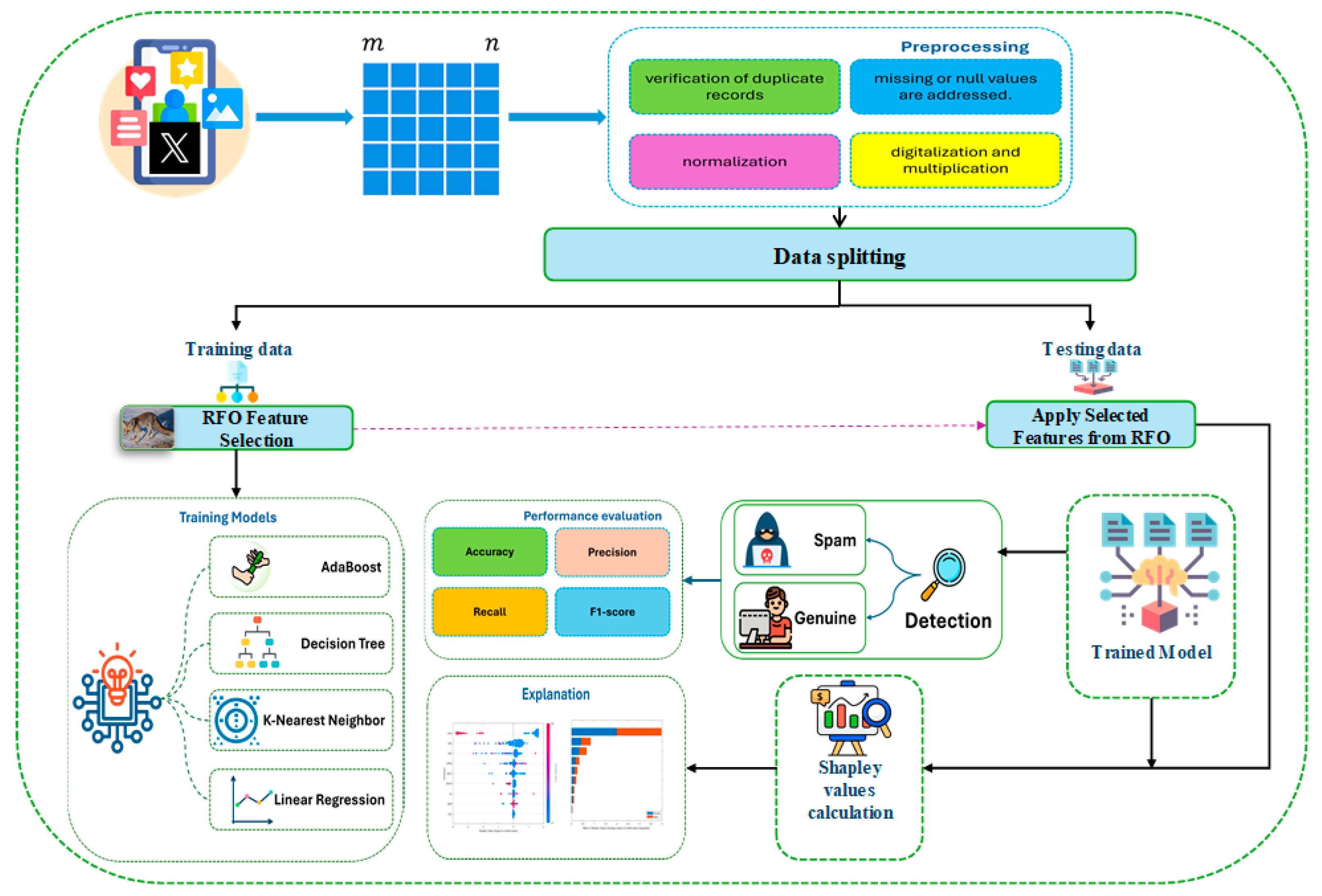
This section delineates the comprehensive approach, as shown in Figure 4., applied in solving the complex problem of X spam account identification. This section begins with the characteristics of the dataset and training and testing subsets. This is then succeeded by a discussion of data preprocessing strategies to guarantee framework stability. The dataset was divided into training and testing subsets. During training, feature selection was performed using RFO, and the selected features were used to train ML models. The same set of selected features was then applied to the testing subset to ensure consistent evaluation.

This section includes a thorough assessment of model efficiency, utilizing various measures for an in-depth evaluation of the model’s value. Ensemble learning integrates multiple models to construct a more robust and accurate classifier [40]. Among these approaches, the boosted trees method—an ensemble technique that combines decision trees as base learners—offers a distinctive advantage in enhancing classification precision. This method effectively captures subtle distinctions that differentiate spam from legitimate accounts [41,42]. The Decision Tree algorithm, in particular, was chosen for its strong capability to handle heterogeneous and high-dimensional feature spaces commonly found in social media datasets. Its hierarchical splitting mechanism efficiently models nonlinear feature interactions while exhibiting resilience to noisy and imperfect input data.

Furthermore, this study provides comparison methods that provide a broader framework to assess the efficacy of the model. The approach has been improved by recent strategies, providing models that explain prediction mechanisms.

4.1. Dataset Description

The dataset used to conduct this study was compiled by the authors of [35]. This dataset consists of 1225 data points, each representing an X account, encompassing 11 unique features—including categorical and numerical attributes—as detailed in

Table 1. The dataset’s taxonomy and criterion ranges.

No	Input Model Features	Type	Range of Evaluate
1	User Statuses Count (USC)	Integer	0–99, 100–199, …, 1,000,000–1,999,999
2	Sensitive Content Alert (SCA)	Boolean	TRUE(T)/FALSE(F)
3	User Favorites Count (UFC)	Integer	0–9, 10–19, 20–29, …, 100,000–1,999,999
4	User Listed Count (ULC)	Integer	0–9, 10–19, 20–29, …, 900–999
5	Source in Twitter (SITW)	String	Yes(Y)/No(N)
6	User Friends Counts (UFRC)	Integer	0–9, 10–19, 20–29, …, 1000–99,999
7	User Followers Count (UFLC)	Integer	0–9, 10–19, 20–29, …, 100,000–1,999,999
8	User Location (UL)	String	Yes(Y)/No(N)
9	User Geo-Enabled (UGE)	Boolean	TRUE(T)/FALSE(F)
10	User Default Profile Image (UDPI)	Boolean	TRUE(T)/FALSE(F)
11	Re-Tweet (RTWT)	Boolean	TRUE(T)/FALSE(F)
12	CLASS	Boolean	TRUE(T)/FALSE(F)

. These attributes encapsulate account characteristics, user behavior, and X metadata. This set contains 718 accounts classified as spam accounts, while the remaining 507 are legitimate users labeled as non-spam. This establishes a dependable benchmark for the classification of spam versus non-spam accounts. The dataset encompasses a combination of user profile attributes and X post-level metrics that are effective in differentiating spammers from authentic users.

The categorical criteria for features in the utilized dataset are detailed as follows:

• User Profile Features: Several attributes measure account activity. The user statuses count (USC) represents the user’s latest tweets or retweets, indicating the account’s productive activity on the platform. Moreover, user followers count (UFLC) represents the total quantity of tweets this user has endorsed throughout the account’s existence. In contrast, user friends count (UFRC) represents the number of users following the account, which is also known as their “followings”. The user favorites count (UFC) shows whether the verifying user has liked (favorited) a tweet. Additionally, the user listed count (ULC) indicates the number of public lists of which the user is a member, measuring the account’s prominence among other users. These indicators essentially encapsulate the engagement of accounts and their footprint in social platforms. The inclusion of these properties enables the analysis of such patterns within the dataset.
• Tweet and Profile Indicators: Datasets additionally include a binary number (yes/no) attribute that represents tweet characteristics and profile configurations. Sensitive Content Alert (SCA) represents a Boolean value, denoting sensitive items contained in the tweet’s content or within the textual user properties. This may indicate spam, as spam tweets often contain this type of content. Source-in-X (SITW) displays the utility employed to publish the tweet, and it is formatted as an HTML string. It denotes whether the tweet was disseminated using an official X platform (YES) or a third-party source (NO). For instance, tweets originating from the X website have a source designation of web. Conversely, spammers may utilize specific applications. User location (UL) constitutes a category domain, indicating the user-provided location for the account’s profile. If the location is provided, then the text is YES; otherwise, an unfilled value is denoted by NO. The location’s actual text is not employed due to its random nature and parsing difficulty. This binary characteristic only indicates the existence of a profile’s location, as is commonly possessed by legal users. User geo-enabled (UGE) indicates whether the user has activated geotagging on tweets (if yes, it is designated as TRUE, indicating that the account permits the attachment of geographical coordinates to tweets). The user default profile image (UDPI) is a Boolean variable, and it signifies that the user is using the default X profile picture (when true, it indicates that the user has not uploaded an image for the profile). For a significant proportion of accounts, suspicious accounts typically use the default image profile and provide minimal private information [42]. Thus, this characteristic may indicate a potential threat. Finally, the ReTweet (RTWT) Boolean value indicates whether the validating user has retweeted a tweet.
• Class Attribute: This attribute signifies that an account is categorized as a spam account if true, while a false designation signifies that the account is legal.

Overall, this dataset offers a comprehensive overview of X account attributes, integrating user profile metrics with content indicators. The fundamental reason for providing an extensive overview of the data is the essential need to thoroughly understand the dataset’s intricacies prior to initiating ML models. This is essential for constructing a robust spam identification system.

4.2. Data Preprocessing and Balancing

This section discusses the preprocessing operations conducted on the X spam dataset to prepare the proposed model. The objective consists of data cleansing, addressing any anomalies, and converting the data into a structure that fits ML techniques. The procedure started with the verification of duplicate records, which could be present as a result of the challenges faced when collecting data. Following this step, every single row constitutes a distinct data element. Subsequently, missing or null values are addressed. Although such elements are infrequent, they are excluded to prevent bias during the subsequent scaling process. Following stage is data digitalization. All binary features are encoded with “Yes-No” values or Boolean “True-False” values, which are then transformed into numerical values: “1–0”.

To prevent information leakage from near-identical samples, we implemented a tiered cross-validation framework with group-aware outer splits based on the account’s identifier. The outer loop employed GroupKFold, ensuring that instances from the same account were never allocated to both training and test folds. We additionally implemented this requirement programmatically by confirming the lack of ID overlap before model assessment. The dataset was neither globally augmented nor expanded before splitting; instead, the only augmentation method employed was SMOTE, which was applied exclusively to the training subsets of the inner cross-validation. This solution guarantees that resampling does not compromise validation or test sets and conforms to recommended practices for preventing leakage in scenarios with possible near-duplicate observations.

Numerous input variables were provided by the data supplier in broad numeric ranges (e.g., “0–9”, “10–19”, …, “100,000–1,999,999”). To achieve a continuous representation without introducing extraneous stochasticity, we assigned each interval to its midpoint and utilized this value in the learning pipeline. This transformation maintains the ordinal arrangement of the bins, permits standard preprocessing (median imputation and normalization), and enhances model-agnostic interpretability.

Every row represents the 11 input unique features, five normalized continuous elements (indicating the user’s status count, follower count, etc.), six binary indicators (for indicators such as sensitive content, default picture, etc.), and finally, the binary class label.

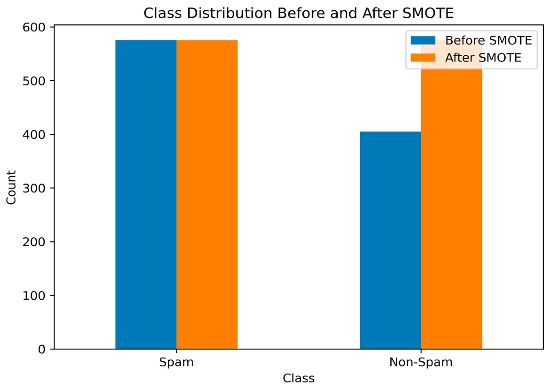
The clean dataset of 1225 samples was split into two subsets with respect to an 80:20 ratio for model training and testing. Due to the intrinsic class imbalance, SMOTE is utilized only on training folds within the cross-validation framework, and it is neither fitted nor applied to the associated validation/test data. This technique guarantees that resampling does not modify the empirical class distribution in the held-out folds and that all provided class-specific measures accurately represent performance with respect to the original test data [43]. Via the execution of these preprocessing activities, the detection models are able to make efficient use of information without being hindered during the process. These careful preprocessing steps provide a solid foundation for building an accurate spam detection model. Figure 5 shows the SMOTE class distributions.

4.3. Feature Selection Approach

Feature selection is an essential process within ML that significantly impacts model efficacy. Not every feature within a dataset inherently aids the model’s training procedure. Extraneous features might diminish the model’s ability to carry out classification, thus impeding the learning phase. Selecting the best feature subset that beneficially impacts the model streamlines it, facilitating the achievement of more precise and expedited outcomes.

4.4. Rüppell’s Fox Optimization

In ML domains, traditional optimization techniques frequently face difficulties due to the expansive and intricate solution spaces encountered. Meta-heuristic methods provide efficient solutions for addressing this constraint. These algorithms apply random search techniques to locate solutions near the global optimum. Meta-heuristic techniques, occasionally inspired by natural events, are especially beneficial for selection feature tasks because of their low computing expense and excellent precision. This study leverages RFO—a swarm-based algorithm inspired by the hunting and survival behaviors of Rüppell’s foxes, for feature selection. The RFO algorithm systematically balances local exploitation with global exploration to ascertain optimal solutions. It begins with randomness-based steps to investigate various areas and amplifies its search with respect to the most promising answers to expedite convergence. RFO creates random initial positions in each dimension after establishing the upper and lower boundaries of the solution space, as shown via Equations (1)–(3). The population size, maximum iterations, and algorithm-specific parameters are established during this stage. After determining the lower and upper bounds of the solution space, RFO generates random starting positions in each dimension. Its equation is given as follows:

$$y_j^i=l_j+r\times \left(u_j-l_j\right)$$

(1)

• $y_j^i:j\mathrm{t}\mathrm{h} \mathrm{d}\mathrm{i}\mathrm{m}\mathrm{e}\mathrm{n}\mathrm{s}\mathrm{i}\mathrm{o}\mathrm{n}\mathrm{a}\mathrm{l} \mathrm{c}\mathrm{o}\mathrm{o}\mathrm{r}\mathrm{d}\mathrm{i}\mathrm{n}\mathrm{a}\mathrm{t}\mathrm{e} \mathrm{o}\mathrm{f} \mathrm{t}\mathrm{h}\mathrm{e} \mathrm{i}\mathrm{t}\mathrm{h} \mathrm{m}\mathrm{e}\mathrm{m}\mathrm{b}\mathrm{e}\mathrm{r} \mathrm{w}\mathrm{i}\mathrm{t}\mathrm{h}\mathrm{i}\mathrm{n} \mathrm{t}\mathrm{h}\mathrm{e} \mathrm{p}\mathrm{o}\mathrm{p}\mathrm{u}\mathrm{l}\mathrm{a}\mathrm{t}\mathrm{i}\mathrm{o}\mathrm{n}$
• $u_j: \mathrm{T}\mathrm{h}\mathrm{e} \mathrm{u}\mathrm{p}\mathrm{p}\mathrm{e}\mathrm{r} \mathrm{l}\mathrm{i}\mathrm{m}\mathrm{i}\mathrm{t} \mathrm{o}\mathrm{f} \mathrm{t}\mathrm{h}\mathrm{e} j–\mathrm{t}\mathrm{h} \mathrm{d}\mathrm{i}\mathrm{m}\mathrm{e}\mathrm{n}\mathrm{s}\mathrm{i}\mathrm{o}\mathrm{n}$
• $l_j: \mathrm{T}\mathrm{h}\mathrm{e} \mathrm{l}\mathrm{o}\mathrm{w}\mathrm{e}\mathrm{r} \mathrm{l}\mathrm{i}\mathrm{m}\mathrm{i}\mathrm{t} \mathrm{o}\mathrm{f} \mathrm{t}\mathrm{h}\mathrm{e} j–\mathrm{t}\mathrm{h} \mathrm{d}\mathrm{i}\mathrm{m}\mathrm{e}\mathrm{n}\mathrm{s}\mathrm{i}\mathrm{o}\mathrm{n}.$
• $r: \mathrm{A} \mathrm{r}\mathrm{a}\mathrm{n}\mathrm{d}\mathrm{o}\mathrm{m} \mathrm{n}\mathrm{u}\mathrm{m}\mathrm{b}\mathrm{e}\mathrm{r} \mathrm{g}\mathrm{e}\mathrm{n}\mathrm{e}\mathrm{r}\mathrm{a}\mathrm{t}\mathrm{e}\mathrm{d} \mathrm{w}\mathrm{i}\mathrm{t}\mathrm{h}\mathrm{i}\mathrm{n} \mathrm{t}\mathrm{h}\mathrm{e} \mathrm{i}\mathrm{n}\mathrm{t}\mathrm{e}\mathrm{r}\mathrm{v}\mathrm{a}\mathrm{l} \left[0,1\right].$

The daytime mode is designated if p is greater than or equal to 0.5; otherwise, the nighttime mode is activated. The Rüppell’s fox’s senses and the algorithm’s update techniques during each iteration are determined by the daylight and night modes. The following equations are used to calculate eyesight, hearing, and smell:

$$\mathrm{s}={\displaystyle \frac{1}{1+{\mathrm{e}}^{\left(\mathrm{K}/2-\mathrm{k}\right)/100}}}$$

(2)

$$\mathrm{h}={\displaystyle \frac{1}{1+{\mathrm{e}}^{\left(\mathrm{k}-\mathrm{K}/2\right)/100}}}$$

(3)

$$\mathrm{s}\mathrm{m}\mathrm{e}\mathrm{l}\mathrm{l}={\displaystyle \frac{0.1}{\left|\mathrm{a}\mathrm{c}\mathrm{o}\mathrm{s}\left(\frac{2}{1+{\mathrm{e}}^{\left(\mathrm{K}/2-\mathrm{k}\right)/100}}\right)\right|}}$$

(4)

where $K$ is the maximum iteration, and $k$ is the present iteration. The behavioral strategies are listed in

Table 2. Decision table regarding day–night modes in RFO.

Mod	Mod Selection Criteria (p)	Condition	Update Strategy
Day-time	p ≥ 0.5	s ≥ h, rand ≥ 0.25	Sense of vision (Equation (5))
Day-time	p ≥ 0.5	s ≥ h, rand < 0.25	Eye movement (Equation (6))
Day-time	p ≥ 0.5	s < h, rand ≥ 0.75	Sense of hearing (Equation (7))
Day-time	p ≥ 0.5	s < h, rand < 0.75	Ear movement (Equation (9))
Night-time	p < 0.5	s < h, rand ≥ 0.25	Sense of hearing (Equation (8))
Night-time	p < 0.5	s < h, rand < 0.25	Ear movement (Equation (9))
Night-time	p < 0.5	s ≥ h, rand ≥ 0.75	Sense of vision (Equation (5))
Night-time	p < 0.5	s ≥ h, rand < 0.75	Eye movement (Equation (6))

.

Table 2 shows the decision table. Behavioral strategies in day and night modes are determined by the “rand” threshold. Based on this threshold, the “rand” variable is randomly generated in the range of [0, 1]. The strategies are updated based on the conditions given in Table 2.

The sense of vision is one of the most critical components of the fox’s search strategy. This mechanism allows the individual to update its position in the current solution space based on both the best individual and a randomly selected individual. This allows the fox to perceive its environment relatively and potentially explore better areas. The mathematical update is given in Equation (5):

$$y_{k+1}^i=x_k^i+r_{\mathrm{index}}\times \left(x_{\mathrm{rand}}-x_k^i\right)+r_{\mathrm{index}}\times \left(fbes{t}_k-x_k^i\right)$$

(5)

• $y_{k+1}^i:\mathrm{N}\mathrm{e}\mathrm{w} \mathrm{l}\mathrm{o}\mathrm{c}\mathrm{a}\mathrm{t}\mathrm{i}\mathrm{o}\mathrm{n}$
• $x_{k+1}^i:\mathrm{C}\mathrm{u}\mathrm{r}\mathrm{r}\mathrm{e}\mathrm{n}\mathrm{t} \mathrm{l}\mathrm{o}\mathrm{c}\mathrm{a}\mathrm{t}\mathrm{i}\mathrm{o}\mathrm{n}$
• $x_{\mathrm{rand} }:\mathrm{L}\mathrm{o}\mathrm{c}\mathrm{a}\mathrm{t}\mathrm{i}\mathrm{o}\mathrm{n} \mathrm{o}\mathrm{f} \mathrm{r}\mathrm{a}\mathrm{n}\mathrm{d}\mathrm{o}\mathrm{m} \mathrm{i}\mathrm{n}\mathrm{d}\mathrm{i}\mathrm{v}\mathrm{i}\mathrm{d}\mathrm{u}\mathrm{a}\mathrm{l}$
• $fbes{t}_k:\mathrm{P}\mathrm{o}\mathrm{s}\mathrm{i}\mathrm{t}\mathrm{i}\mathrm{o}\mathrm{n} \mathrm{o}\mathrm{f} \mathrm{t}\mathrm{h}\mathrm{e} \mathrm{b}\mathrm{e}\mathrm{s}\mathrm{t} \mathrm{i}\mathrm{n}\mathrm{d}\mathrm{i}\mathrm{v}\mathrm{i}\mathrm{d}\mathrm{u}\mathrm{a}\mathrm{l}$
• $r_{\mathrm{index}}:\left[0,1\right] \mathrm{r}\mathrm{a}\mathrm{n}\mathrm{d}\mathrm{o}\mathrm{m} \mathrm{c}\mathrm{o}\mathrm{e}\mathrm{f}\mathrm{f}\mathrm{i}\mathrm{c}\mathrm{i}\mathrm{e}\mathrm{n}\mathrm{t} \mathrm{i}\mathrm{n} \mathrm{t}\mathrm{h}\mathrm{e} \mathrm{r}\mathrm{a}\mathrm{n}\mathrm{g}\mathrm{e}$

Here, $y_{k+1}^i$ represents the updated position of the individual; $x_{k+1}^i$ represents the current position; $x_{\mathrm{rand} }$ represents the position of a randomly selected individual from the population; $fbes{t}_k$ represents the position of the best individual obtained in the relevant iteration.

Eye movement refers to the fox’s observation of its environment, updating its position by referencing both random individuals and the best individual. It mimics the fox’s assessment of potential opportunities in its environment through visual perception. This is described via Equation (6):

$$y_{k+1}^i=y_{\mathrm{rotate}}^i+\mathsf{\beta }\times randn\left(1,d\right)\times flag$$

(6)

• $y_{rotate}^i:\mathrm{R}\mathrm{o}\mathrm{t}\mathrm{a}\mathrm{t}\mathrm{e}\mathrm{d} \mathrm{p}\mathrm{o}\mathrm{s}\mathrm{i}\mathrm{t}\mathrm{i}\mathrm{o}\mathrm{n} \mathrm{v}\mathrm{e}\mathrm{c}\mathrm{t}\mathrm{o}\mathrm{r}$
• $\mathsf{\beta }:\mathrm{S}\mathrm{c}\mathrm{a}\mathrm{l}\mathrm{i}\mathrm{n}\mathrm{g} \mathrm{f}\mathrm{a}\mathrm{c}\mathrm{t}\mathrm{o}\mathrm{r}$
• $randn\left(1,d\right):d-\mathrm{d}\mathrm{i}\mathrm{m}\mathrm{e}\mathrm{n}\mathrm{s}\mathrm{i}\mathrm{o}\mathrm{n}\mathrm{a}\mathrm{l} \mathrm{v}\mathrm{e}\mathrm{c}\mathrm{t}\mathrm{o}\mathrm{r} \mathrm{r}\mathrm{a}\mathrm{n}\mathrm{d}\mathrm{o}\mathrm{m}\mathrm{l}\mathrm{y} \mathrm{g}\mathrm{e}\mathrm{n}\mathrm{e}\mathrm{r}\mathrm{a}\mathrm{t}\mathrm{e}\mathrm{d}$
• $flag:\mathrm{R}\mathrm{a}\mathrm{n}\mathrm{d}\mathrm{o}\mathrm{m} \mathrm{v}\mathrm{a}\mathrm{r}\mathrm{i}\mathrm{a}\mathrm{b}\mathrm{l}\mathrm{e}\left(+1 or -1\right)$
• $d:\mathrm{D}\mathrm{i}\mathrm{m}\mathrm{e}\mathrm{n}\mathrm{s}\mathrm{i}\mathrm{o}\mathrm{n} \mathrm{o}\mathrm{f} \mathrm{t}\mathrm{h}\mathrm{e} \mathrm{s}\mathrm{o}\mathrm{l}\mathrm{u}\mathrm{t}\mathrm{i}\mathrm{o}\mathrm{n} \mathrm{s}\mathrm{p}\mathrm{a}\mathrm{c}\mathrm{e}$

Here, $y_{rotate}^i$ represents the individual’s rotated position, enabling the search for the current solution in different directions. The $\mathsf{\beta }$ coefficient controls the step size, while $randn\left(1,d\right)$ creates random variations, helping individuals avoid local optima. The $flag$ parameter determines the direction of movement, simulating eye shifts from the right to the left.

Hearing is a mechanism that simulates a fox’s position updates by detecting sound sources within its environment. In this approach, the individual orients itself toward both the location of a randomly selected individual and the best individual in the population. Thus, the fox gains the ability to explore new regions in the solution space using sensory perception.

In the daytime mode, the individual’s location is updated via a randomly selected individual $(x_{\mathrm{rand}}$), while in the nighttime mode, this process differs, and the individual moves toward the location of another individual ${(y}_{\mathrm{rand}}$). This is described in Equations (7) and (8).

$$y_{k+1}^i=x_k^i+r_{\mathrm{index}}\times \left(x_{\mathrm{rand}}-x_k^i\right)+r_{\mathrm{index}}\times \left(fbes{t}_k-x_k^i\right) \mathrm{In\; day\; mode}$$

(7)

$$y_{k+1}^i=x_k^i+r_{\mathrm{index}}\times \left(y_{\mathrm{rand}}-x_k^i\right)+r_{\mathrm{index}}\times \left(fbes{t}_k-x_k^i\right) \mathrm{In\; night\; mode}$$

(8)

$y_{\mathrm{rand}} \mathrm{d}\mathrm{e}\mathrm{n}\mathrm{o}\mathrm{t}\mathrm{e}\mathrm{s} \mathrm{t}\mathrm{h}\mathrm{e}: random location of different individuals$. All other variables are the same as in Equation (5).

Ear movement is an updating mechanism that mimics the fox’s behavior of perceiving sounds in its environment and adjusting its direction accordingly. This mechanism is formulated in Equation (9).

$$y_{k+1}^i=y_{\mathrm{rotate}}^i+\mathsf{\beta }\times randn\left(1,d\right)\times flag$$

(9)

All variables are the same as in Equation (6).

Additionally, the sense of smell is a critical component of foxes’ environmental perception—it is a search strategy. This mechanism allows individuals to update their position in the current solution space based on both the best individual and a randomly selected individual. By sniffing their environment, foxes gain the ability to explore new areas and can also navigate to the best known solution. This updating process is expressed via Equation (10).

$$y_{k+1}^i=\left\{\begin{array}{c}{x}_k^i+\rho \times \left(x_{rand1}-x_k^i\right)\times r_2\\ +\rho \times \left(fbes{t}_k-x_k^i\right)\times r_3 r_1\ge smell\\ x_{rand1}+\beta ·randn\left(1,d\right) r_1<smell\end{array}\right.$$

(10)

Here, $x_k^i$ represents the current individual’s location; $fbes{t}_k$ represents the best individual’s location; $x_{rand1}$ represents the location of a randomly selected individual from the population. If the $r_1\ge smell$ condition is met, the individual gravitates toward both the best solution and a randomly selected individual, which is called exploitation behavior. Otherwise, if the $r_1<smell$ condition is met, the individual is shifted to a completely random position. This allows foxes to diversify their solution space and avoid local minima.

Another important component of fox herding behavior is the best individual orientation mechanism. This mechanism ensures that individuals in the population continually converge toward the best solution, thus increasing the algorithm’s convergence rate. This phenomenon is described in Equation (11).

$$y_{k+1}^i=\left\{\begin{array}{c}{x}_k^i+c_0\times \left(x_{rand}-x_k^i\right)\times r_1\\ +c_1\times \left(fbes{t}_k-x_k^i\right)\times r_2 rand\ge 0.1\\ \left(x_k^i+x_k^i\right)/2 rand<0.1\end{array}\right.$$

(11)

If the random number is $rand\ge 0.1$, the individual is shifted toward both the randomly selected individual and the best solution. However, if $rand<0.1$ is met, the individual is pulled to an average point close to its current location, preventing excessive deviations.

An additional mechanism is defined in the algorithm to update the worst individuals. This step prevents the weakest individuals in the population from slowing down the herd’s progress. This is described in Equation (12).

$$y_{k+1}^{\mathrm{worst}}=y_k^{\mathrm{worst}}+\mathsf{\beta }\times \mathrm{randn}\left(1,d\right)\hspace{1em}flag=1$$

(12)

With random updates based on normal distributions, the worst individual is repositioned in the solution space, which prevents the population from concentrating at a single point and allows the search to spread over a wider solution space. The pseudocode of the RFO algorithm used is provided below (Algorithm 1).

Algorithm 1. Pseudocode of the Rüppell’s Fox optimizer (RFO).

1    Define the problem configuration and initialize RFO 2    Determine the initial population’s positions 3    while (k < K) do 4    if (p − 0.5) ≥ 0 then 5    for i = 1 to n do 6    if (s ≥ h) then 7    if (rand ≥ 0.25) then 8    Update the position of Rüppell’s foxes in daylight through the sense of sight Equation (5). 9    else 10  Update the position of Rüppell’s foxes in daylight through the eye-rotation mecha-nism Equation (9). 11  end if 12  else 13  if (rand ≥ 0.75) then 14  Update the position of Rüppell’s foxes in daylight through the sense of hearing Equation (7). 15  else 16  Update the position of Rüppell’s foxes in daylight through the ear-rotation mecha-nism Equation (9). 17  end if 18  end if 19  end for 20  else 21  for i = 1 to n do 22  if (s < h) then 23  if (rand ≥ 0.25) then 24  Update the position of Rüppell’s foxes at night through the sense of hearing Equation (8). 25  else 26  Update the position of Rüppell’s foxes at night through the ear-rotation mechanism Equation (9). 27  end if 28  else 29  if (rand ≥ 0.75) then 30  Update the position of Rüppell’s foxes at night through the sense of sight Equation (5). 31  else 32  Update the position of Rüppell’s foxes at night through the eye-rotation mechanism Equation (6). 33  end if 34  end if 35  end for 36  end if 37  for i = 1 to n do 38  if (rand ≥ smell) then 39  Update the position of Rüppell’s foxes through the sense of smell Equation (10) (First-case). 40  else 41  Update the position of Rüppell’s foxes through the sense of smell Equation (10) (Second-case). 42  end if 43  end for 44  for i = 1 to n do 45  if (rand ≥ 0.1) then 46  Update the position of Rüppell’s foxes towards the best one Equation (11) (First-case). 47  else 48  Update the position of Rüppell’s foxes towards the best one Equation (11) (Second-case). 49  end if 50  end for 51  for i = 1 to n do 52  if (flag == 1) then 53  Update the position of Rüppell’s foxes in the worst case of exploration Equation (12). 54  end if 55  end for 56  k = k + 1 57  end while 58  Report the best solution identified so far.

To prevent the leakage of information during feature selection, we employed a nested cross-validation framework, where the RFO-based selector was integrated as a transformer step within the machine learning pipeline. In each outer split, the data were partitioned in a group-aware manner according to the account identifier (ID), ensuring that no records from the same account appeared simultaneously in the training and test folds. Within each outer training fold, the RFO selector was exclusively fitted on the training partitions and optimized using K-nearest neighbor (k = 5), and its accuracy was assessed via inner cross-validation. The selected features were subsequently fixed before evaluating the downstream classifier on the held-out outer test fold. Throughout this process, no preprocessing, resampling, feature selection, or hyperparameter tuning was involved in the external test fold. This design ensures that the reported performance estimates faithfully represent generalization to unseen accounts while mitigating biases induced by feature selection. The features ultimately retained by the RFO algorithm are presented in

Table 3. Features selected by the RFO algorithm.

Optimal Features	Selected Features
Nine optimal features for detection models	SCA, UL, UDPI, RTWT, USC, UFC, ULC, UFRC, and UFLC
Eleven optimal features for detection models	Statuses_count, default_profile, profile_banner_url, favourites_count, geo_enabled, location, friends_count, description, followers_count, fav_number, and listed_count

.

The features listed in Table 3 were identified—using the RFO algorithm—as the most influential features in maximizing classification performance.

4.5. Model Training

This study introduces an RFO dimensionality reduction framework for developing a lightweight, interpretable machine learning spam detection system. This is carried out by identifying the most informative features prior to classifier training. Raw data are first subjected to the preprocessing pipeline detailed in Section 4.2 to ensure consistency for downstream learning. The resulting feature is then passed to the RFO module, as outlined in Section 4.3. For our spam detection task, RFO converges on a feature subset, thereby eliminating redundant variables and simplifying the subsequent classifier without sacrificing performance.

In this study, a lightweight explainable spam detection model is trained using AdaBoost, DT, LR, and KNN ML algorithms; these were optimized using uniform inner cross-validation conditions within the same pipeline framework, and the selected hyperparameters were recorded for each outer test assessment in

Table 4. All model hyperparameter details.

Model Name	Hyperparameter Details
DT	Depth was explored at three and five with an unrestricted upper bound; the minimum split size was evaluated at two, five, and ten. All other settings followed conventional defaults: Gini impurity with best-first splitting, single-sample leaves, no limits on features or leaf nodes, a zero impurity-decrease threshold, no cost–complexity pruning, and no class weighting.
AdaBoost	Ensemble capacity was tuned by exploring one hundred fifty, three hundred, and five hundred learners with learning rates of 0.5 and 1.0; depth-one tree and the real AdaBoost variant was used.
Logistic Regression	optimization with up to two thousand iterations and ridge regularization; inverse regularization strength examined at 0.1, 1.0, and 10.0; a convergence tolerance of ten to the power of minus four, an intercept term included, automatic multiclass handling, no class weighting.
KNN	Neighborhood sizes studied at five, eleven, and twenty-one with uniform and distance-based weighting; Minkowski distance with power two corresponding to Euclidean geometry; the search algorithm selected automatically with a leaf size of thirty.

. This method has been employed by numerous researchers [44,45,46] in investigations on spam and fraud detection.

4.6. Model Evaluation

Machine learning model performance evaluation is an essential stage within a comprehensive model workflow. The evaluation stage includes various types of key metrics, which are crafted to provide an advanced overview of a model’s strengths and constraints, thus directing future endeavors to enhance prediction accuracy. Regarding our study, we chose to apply a set of primary metrics. In order to comprehensively evaluate a model’s efficiency with respect to classification techniques employed in spam detection, the accuracy, F1 score, recall, precision, ROC curve, and AUC are investigated, as shown in

Table 5. Performance metrics for evaluating models.

Metrics	Formula	Description
Accuracy	${\displaystyle \frac{TP+TN}{TP+TN+FP+FN}}$	This is a measure that indicates the proportion of accurately identified cases relative to the total number of cases assessed.
F1 score	$2\times {\displaystyle \frac{Precision\times Recall}{Precision+Recall}}$	This is a statistic that provides the harmonic average of the recall and precision metrics.
Recall	${\displaystyle \frac{TP}{TP+FN}}$	This indicator quantifies the proportion of non-spam positives identified by the training model in a specific classification instance.
Precision	${\displaystyle \frac{TP}{TP+FP}}$	This is a measure that quantifies the proportion of accurately identified positive cases among all positively classified cases. The number of accurate predictions relative to all correct predictions is termed precision.
AUC	$\int TPR\left(FPR\right)\hspace{0.17em}dFPR$	This indicator evaluates the efficacy of the training model based on the ROC curve, illustrating the relationship among the rate of false positives and the rate of true positives across various thresholds.
Macro-average	${\displaystyle \frac{1}{N}}{\displaystyle \sum _{i=1}^N}{M}_i$	Unweighted average metric values per class.
Micro-average	${\displaystyle \frac{{\sum }_{i=1}^{N}T{P}_i}{{\sum }_{i=1}^N\left(T{P}_i+F{P}_i\right)}}$	Average of the designated metric computed from the combined predicted and actual values across all classes.
Weighted average	${\displaystyle \frac{{\sum }_{i=1}^N{w}_i\cdot M_i}{{\sum }_{i=1}^N{w}_i}}$	Weighted average of per-class metric values based on the frequency of occurrence for each class.

.

The following definitions are provided:

• True Positive (TP): This represents the number of accounts the model predicted correctly as spam.
• True Negative (TN): This represents the number of accounts the model predicted correctly as non-spam.
• False Positive (FP): This represents the number of non-spam accounts the model predicted as spam.
• False Negative (FN): This represents the number of spam accounts the model predicted as non-spam.
• TPR (Recall): ${\displaystyle \frac{TP}{TP+FN}}$.
• False Positive Rate (FPR): ${\displaystyle \frac{FP}{FP+TN}}$.
• $M_i$: The metric value for class $i$; $N$: number of classes.
• $T{P}_i$: True positives for class $i$; $F{P}_i$: false positives for class $i$.
• $w_i$: The number of samples belonging to class $i$.

4.7. Implementation Environment

In this study, computing resources were carefully prepared to meet demanding requirements. The hardware resource configuration was based on a personal computer equipped with an Intel (R) Core (TM) i7-14700HX-2.10 GHz CPU with 32 GB of RAM. For the operating system, Windows 11 Pro (64-bit) was used, guaranteeing reliable and effective computational performance. This study employed the Python 3.11.7 programming language, augmented by numerous libraries such as Pandas and NumPy for manipulating data and producing efficient numerical operations. Anaconda was utilized as a platform for environmental management. All experiments were conducted using predetermined random seeds. The precise outer train/test indices were recorded, and run information (paths, seeds, and timestamps) was documented to ensure accurate replication and traceability.

5. Results and Discussion

Our findings indicate the efficacy of explainable ML models in identifying spam accounts on online social networks such as X. This section clarifies the conclusions obtained through the experiments performed within the methodology of this study. The proposed framework with RFO feature selection isolates a feature subset. A reduction to only features is essential for real-time spam systems. By relying on a minimal yet highly discriminative feature set, our classifiers can accurately distinguish spam from legitimate accounts. Moreover, this dimensionality reduction enables a rigorous assessment of our lightweight detection pipeline’s efficiency under practical deployment scenarios. Leveraging the features selected by our RFO framework, we trained four classifiers to construct a lightweight, interpretable spam detection system: AdaBoost, DT, LR, and KNN. All algorithms were evaluated using five-fold GroupKFold cross-validation. Under evaluation (spam and non-spam), the DT, KNN, AdaBoost, and LR models achieved accuracies of 99.10%, 98.77%, 96.57%, and 92.24%, respectively.

Table 6. Detailed performance of all models.

Model	Acc_mean	Prec_mean	Rec_mean	F1_mean	AUC_mean	AUPRC_mean
DT-RFO	99.10	98.49	1	99.23	99.49	99.40
KNN-RFO	98.77	98.00	1	98.98	99.03	98.90
AdaBoost-RFO	96.57	96.79	97.27	97.02	98.631	98.19
LR-RFO	92.24	91.22	95.90	93.47	96.83	97.25

provides the detailed performances observed. In addition to ROC-AUC, we calculated AUPRC to assess performance within the context of imbalance to evaluate calibration and provide the confusion matrix counts. Together, these diagnostics offer a comprehensive assessment of discriminative capacity and dependability.

To quantify uncertainty and enable rigorous model comparisons, we report mean performance, standard deviation, and two-sided 95% t-confidence intervals across five outer cross-validation folds for each classifier (DT, KNN, AdaBoost, and LR). Confidence intervals were computed using the fold-level metric values.

Table 7. Performance across 5 outer CV folds reported as mean ± SD [95% CI]. Metrics are computed from out-of-fold predictions.

Metric	DT	KNN	AdaBoost	LR
AUC_mean	0.99	0.99	0.99	0.97
AUC_sd	0.01	0.02	0.02	0.02
AUC_t95_lo	0.98	0.97	0.96	0.95
AUC_t95_hi	1.01	1.02	1.01	0.99
AUPRC_mean	0.99	0.99	0.98	0.97
AUPRC_sd	0.01	0.02	0.03	0.02
AUPRC_t95_lo	0.98	0.96	0.95	0.95
AUPRC_t95_hi	1.01	1.02	1.01	0.99
MacroF1_mean	0.99	0.99	0.96	0.92
MacroF1_sd	0.01	0.01	0.02	0.02
MacroF1_t95_lo	0.98	0.97	0.94	0.90
MacroF1_t95_hi	1.00	1.00	0.99	0.94
F1_mean	0.99	0.99	0.97	0.93
F1_sd	0.00	0.01	0.02	0.02
F1_t95_lo	0.99	0.98	0.94	0.92
F1_t95_hi	1.00	1.00	1.00	0.95

summarizes the AUC, AUPRC, and macro-F1. For instance, DT attained an AUC of 0.99 (SD: 0.01; 95% CI: 0.98–1.01), and macro-F1 attained 0.99 (SD: 0.01; 95% CI: 0.98–1.00), whereas LR yielded a macro-F1of 0.92 (SD: 0.02; 95% CI: 0.90–0.94). Presenting the mean ± SD and confidence intervals across outer folds permits the transparent assessment of robustness and effect sizes between models.

While the proposed pipeline already mitigates conventional leakage risks through nested, group-aware cross-validation and integrates SHAP-based attributes alongside class-aware metrics, we further conducted a dedicated feature ablation study to rigorously evaluate robustness. Specifically, we reproducibly excluded metadata features SCA, UDPI, and UL from the design matrix within each outer training fold, followed by complete retraining and the evaluation of the pipeline under the same nested cross-validation procedure. The ablation results are listed below:

• KNN: 83.8% accuracy (±0.027), 92.3% recall, 82.7% precision, and an F1 score of 86.9%.
• DT: 83.8% accuracy (±0.021), 96.7% recall, 79.8% precision, and an F1 score of 87.4%.
• LR: 72.9% accuracy (±0.025), 87.8% recall, 72.2% precision, and an F1 score of 79.2%.
• AdaBoost: 72.8% accuracy (±0.030), 84.7% recall, 73.1% precision, and an F1 score of 78.4%.

These findings confirm that the exclusion of SCA, UDPI, and UL does not undermine the model’s predictive capability. Instead, the models, particularly DT and KNN, preserve strong classification performance, thereby supporting the conclusion that the observed results are not merely artifacts of trivially gameable or label-proximal features.

Under identical experimental conditions, the DT configured with RFO demonstrates materially improved computational efficiency compared to the non-RFO baseline. Specifically, the model’s size is reduced from 58,908 bytes to 30,143 bytes, the peak RAM usage decreases from 300.45 MB to 297.57 MB, and the average inference latency per sample improves from 0.0072 ms to 0.0022 ms. These results confirm that the RFO configuration yields a strictly more lightweight and faster DT than the non-RFO baseline under identical test conditions.

5.1. Evaluation of Performance with the ROC Curve

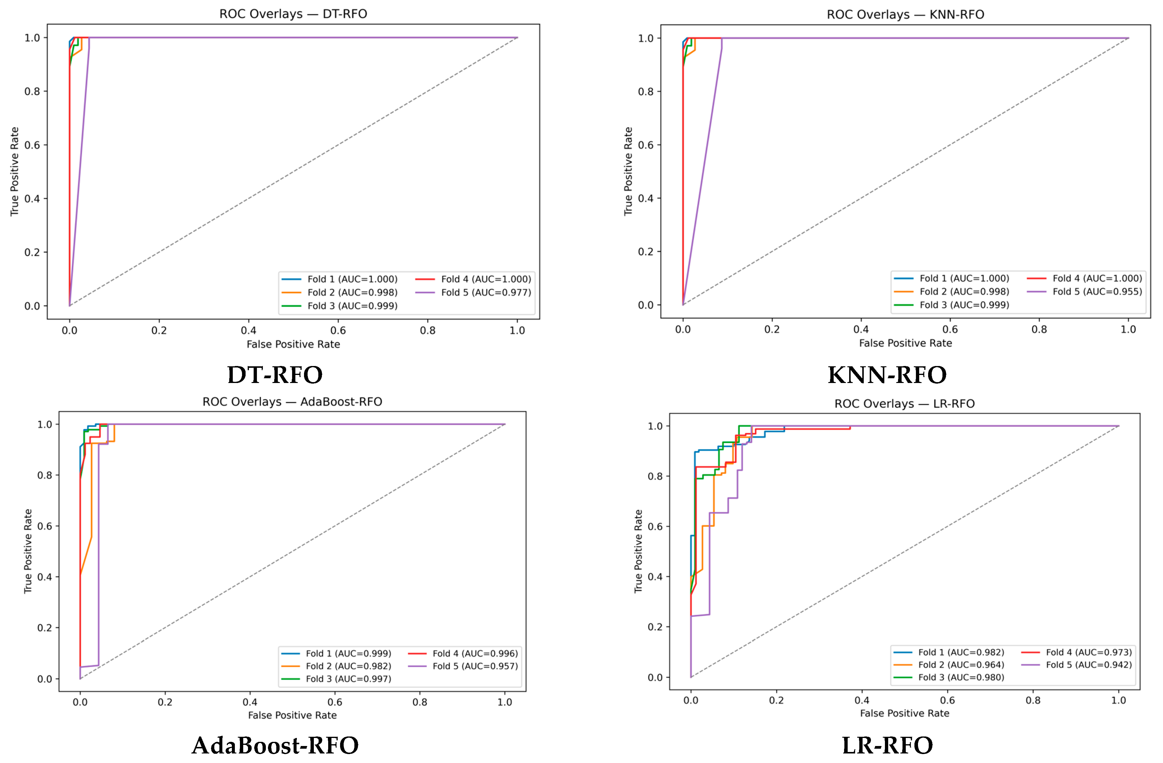
To quantify ML model robustness, we plotted receiver operating characteristic (ROC) curves and computed the area under the curve (AUC) for both spam and non-spam detection. Figure 6 presents (ROC) overlays for four classifiers augmented with RFO-based feature selection, decision tree (DT-RFO), K-nearest neighbor (KNN-RFO), AdaBoost (AdaBoost-RFO), and logistic regression (LR-RFO) across five stratified folds.

DT-RFO and KNN-RFO both achieved perfect discrimination (AUC = 1.000) in three folds and sustained strong performance (AUC = 0.975) in the remaining two folds, highlighting their consistency. AdaBoost-RFO attained uniformly high separability, with AUCs of 0.996 in folds 1 and 3 and 0.975 in folds 4 and 5. LR-RFO exhibited slightly greater variability, with fold AUC values ranging from 0.996 to 0.975, yet it continued to offer robust discrimination well above chance. These overlay plots demonstrate that RFO-driven feature optimization consistently elevates model discriminative power across both tree-based and linear classifiers.

For each outer test fold, we computed the ROC–AUC with nonparametric bootstrap confidence intervals and exported fold-wise metrics to support dispersion reporting across folds. In addition, AUPRC values were recorded to complement discrimination with calibration under class imbalance, as shown in Figure 6 and Table 6.

5.2. Evaluation of Performance with Precision–Recall (PR) and Confidence Intervals (CIs)

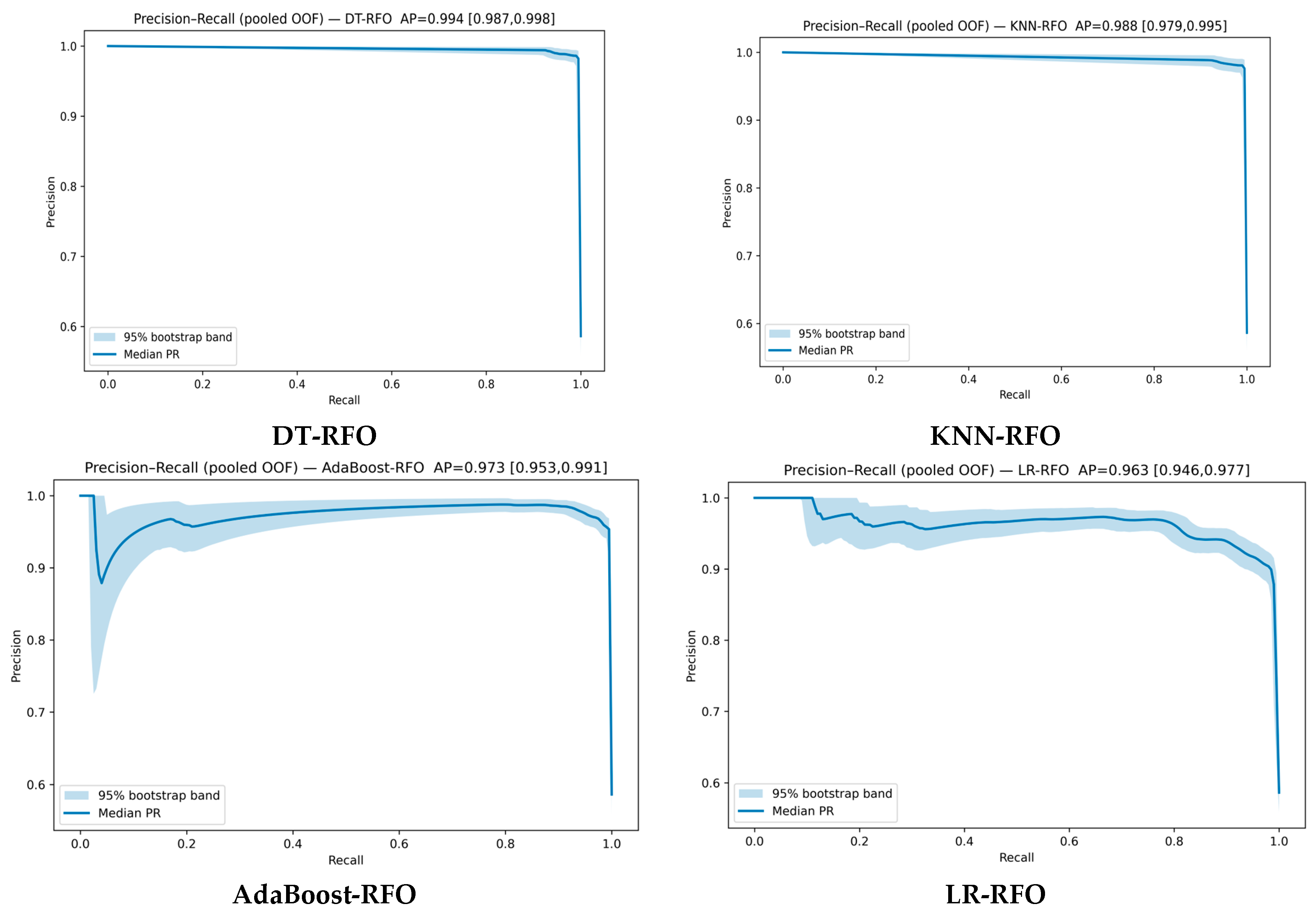
Figure 7 contrasts pooled out-of-fold precision–recall (PR) performance for four RFO-optimized classifiers—decision tree (DT-RFO), K-nearest neighbor (KNN-RFO), AdaBoost (AdaBoost-RFO), and logistic regression (LR-RFO)—with average precision (AP) scores and 95% bootstrap confidence intervals (CIs). The DT-RFO model achieves an AP of 0.994 (CI: 0.987–0.998), maintaining near-perfect precision until recall exceeds 0.9, where it gradually declines. KNN-RFO similarly excels with an AP of 0.988 (CI: 0.979–0.995), sustaining high precision across most recall thresholds. AdaBoost-RFO registers an AP of 0.973 (CI: 0.953–0.991), showing a slight precision dip at low recalls but remaining above 0.8 until the highest recall values. LR-RFO, while slightly lower, still performs robustly with an AP of 0.963 (CI: 0.946–0.977), declining more steadily with increasing recall. These curves underscore that RFO-driven feature selection substantially enhances precision–recall trade-offs, particularly for tree-based models, and that even simpler linear classifiers can achieve competitive PR performance when equipped with optimal feature subsets.

5.3. Performance Evaluation Using a Confusion Matrix

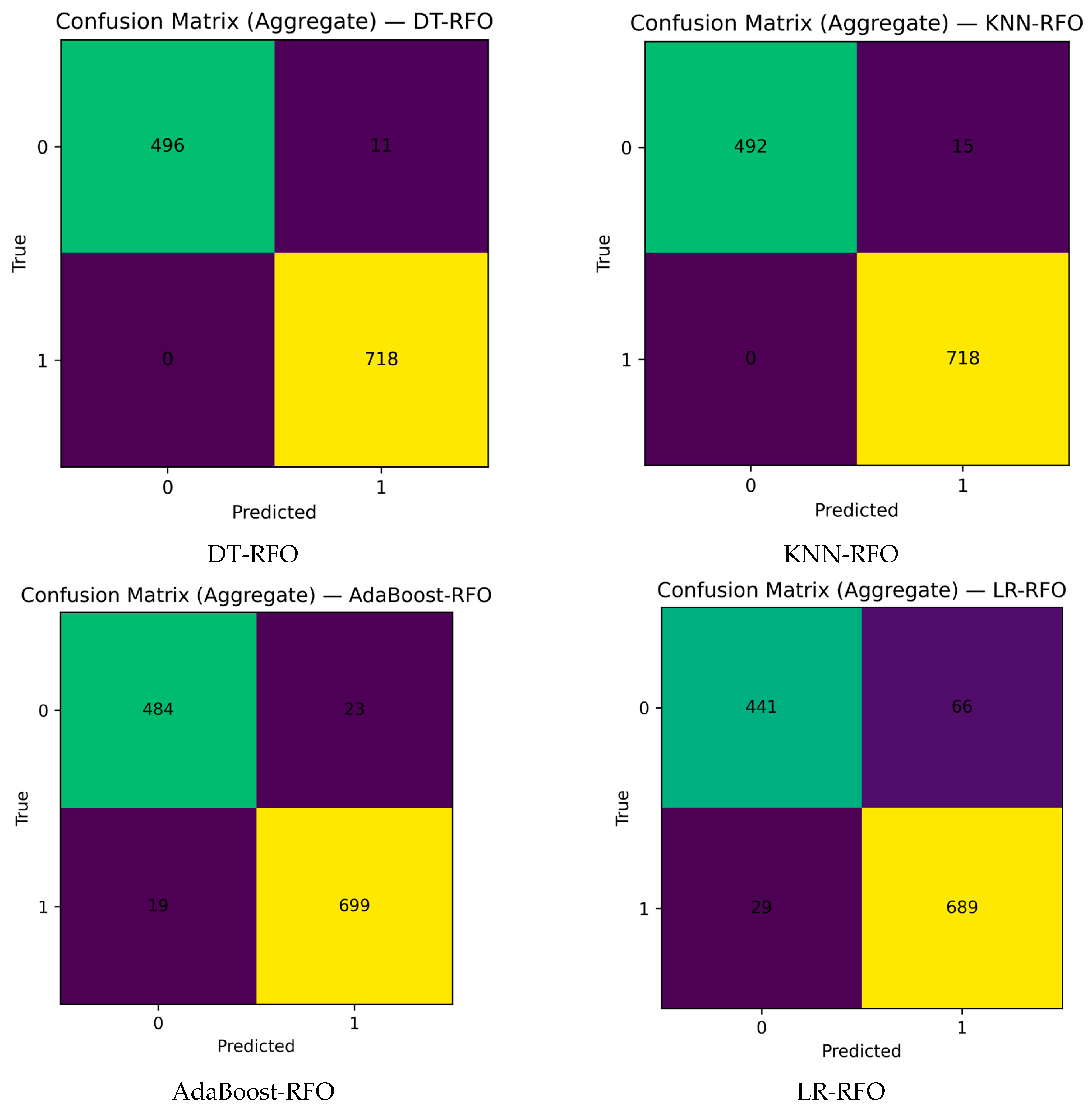
The confusion matrix is used as part of the experimental assessment. Figure 8 summarizes aggregated confusion matrices across stratified folds for four RFO-optimized classifiers—AdaBoost-RFO, LR-RFO, DT-RFO, and KNN-RFO—and highlights their relative strengths in distinguishing spam from legitimate traffic.

AdaBoost-RFO correctly classifies 484 ham and 699 spam messages but incurs 23 false positives and 19 false negatives, achieving specificity and sensitivity above 95%. LR-RFO, by contrast, suffers from greater misclassification—66 ham messages flagged as spam and 29 spam messages missed—reflecting a modest decrease in both specificity (87%) and sensitivity (96%).

DT-RFO eliminates false negatives entirely—capturing all 718 spam samples—and mislabels only 11 of the 507 ham messages, yielding 100% sensitivity and 97.8% specificity. KNN-RFO matches this perfect recall with 0 false negatives and commits only 15 false positive misclassifications, achieving 100% sensitivity and 97.0% specificity.

These results demonstrate that RFO-driven feature selection markedly enhances classifier performance, with tree-based models (DT and KNN) delivering near-perfect detection and minimal ham misclassification, while linear and boosting methods—although strong—remain slightly more prone to errors.

5.4. Explain Global Model Predictions Using Shapley Importance Plot

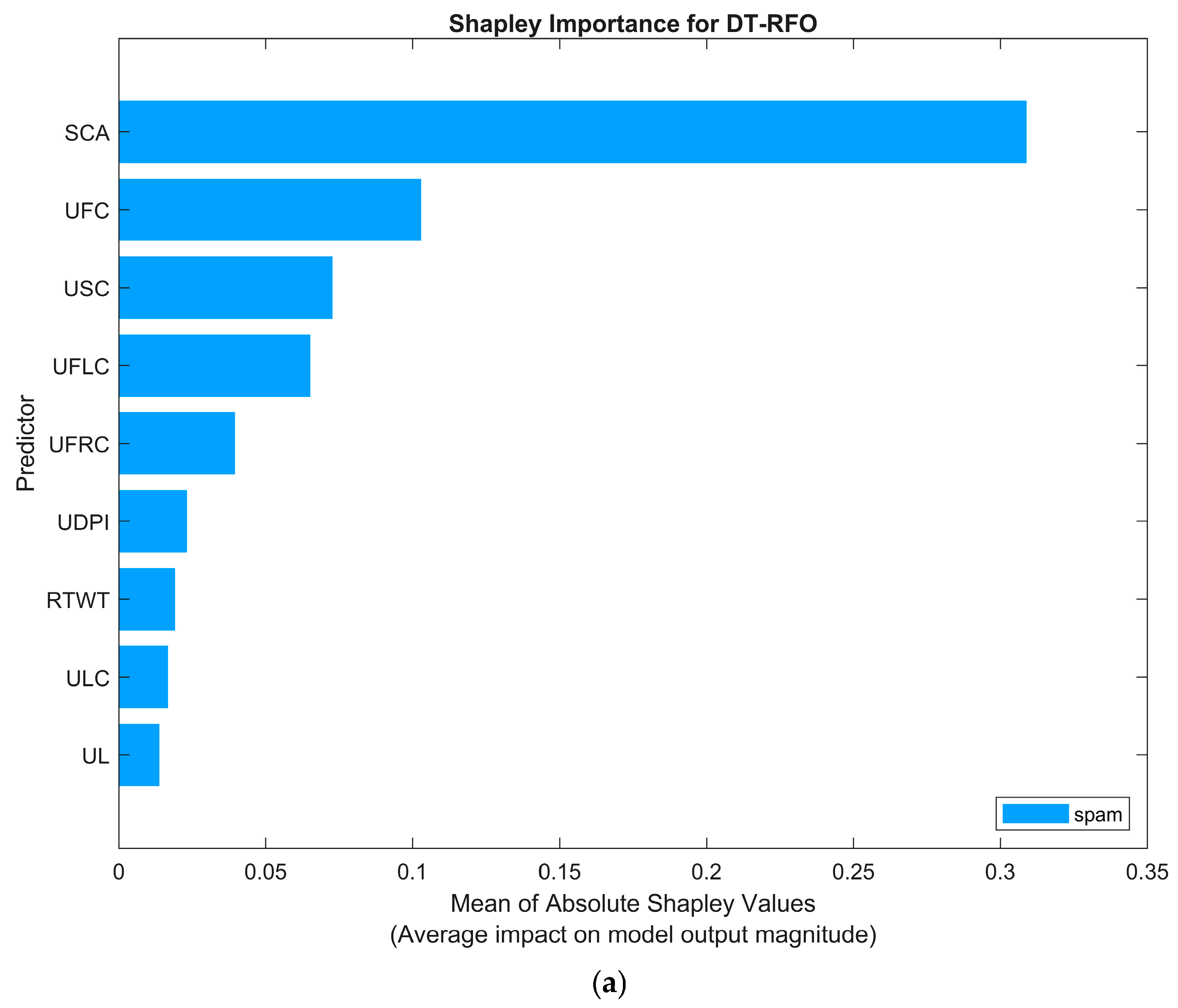
The SHAP analysis depicted in Figure 9a functions as a crucial technique for clarifying the intricate procedures involved in making decisions within the XAI-ROF-DT method. The Shapley importance chart offers a model-agnostic game-theoretic assessment of feature impacts. Such a score becomes crucial for comprehending the impact of each feature on the prediction results.

The Shapley values of predictors for a collection of query points are used to ascertain which predictors exert the most important (or least important) average influence on the size of the model’s output. These values elucidate the divergence of the forecast for the query point from the mean prediction, and they are attributable to the predictor. The sign of the Shapley value denotes the direction of the deviation, while the absolute value signifies its size. This high interpretability degree is essential for models that require significant responsibility and transparency.

Additionally, specific features strongly influence the predicted effectiveness based on the ensemble model. The Shapley importance analysis showed that SCA is the main feature affecting both spam and non-spam prediction scores. In particular, the mean absolute Shapley values demonstrate that altering SCA modifies the expected classification score.

Secondary features such as UFC, USC, and UFRC exhibited a moderate impact, where each predicated spam portion partially surpasses the non-spam portion. This disparity signifies a slightly greater influence on increasing the spam score compared to the non-spam score. UDPI, RTWT, and ULC exerted diminishing effects in succession, while UL had minimal influence.

In conclusion, Shapley importance values highlight that content-based indicators (SCA) and high-level indicators of engagement (USC and UFC) stimulate and reinforce spam identification. These findings underscore their potential for focused feature engineering, specifically enhancing indicators for “sensitive content”, stressing the significance of XAI approaches in transparent and responsible cybersecurity frameworks.

5.5. Explaining Global Model Predictions Using Shapley Summary Plots

In contrast, Shapley swarm charts, as shown in Figure 9b, are employed to comprehend the complexity of the prediction processes in the ML models used in this study. Shapley swarm charts are used to interpret the influence of individual indications with respect to model classification. Positive SHAP values suggest that these features predominantly influence model classification with respect to spam accounts. Conversely, negative values move the model toward non-spam accounts. This deep understanding is essential for situations where explainability and transparency are critical. The features of “SCA”, “UFC”, and “USC” exhibit the greatest positive SHAP values. This indicates that these features are robust markers for categorizing an account as spam. These elevated SHAP values indicate significant influence on the model’s ability to predictions. Low “SCA” features in X accounts generated substantially positive SHAP values, thus elevating spam account identification probabilities. Conversely, high “SCA” was associated with negative SHAP values, significantly steering the model away from classifying accounts as non-spam. The second most impactful feature was “UFC”—accounts with few favorites showing positive values—while active “favorites” yielded negative SHAP values. “USC” is ranked third, as accounts with a minimal number of total tweets (low USC) exhibited positive SHAP values, suggesting an increased probability of spam, while elevated “USC” values yielded negative SHAP scores indicative of non-spam behavior. Features with moderate influence included “UFLC” and “UFRC”. Reduced “UFLC” or “UFRC” with positive SHAP values increases the possibility of spam, whereas elevated tend to inhibit it. Retweet features “RTWT” and “UDPI” exhibited a comparable trend, and the minimal retweet rate moderately inclined closer to spam. In contrast, elevated retweet activity significantly favored non-spam content. ULC” exhibited lower effects; nonetheless, their patterns remained stable. Finally, for “UL”, a valid location and customized avatar marginally reduce the likelihood of spam.

5.6. Comparison with Another X Spam Dataset

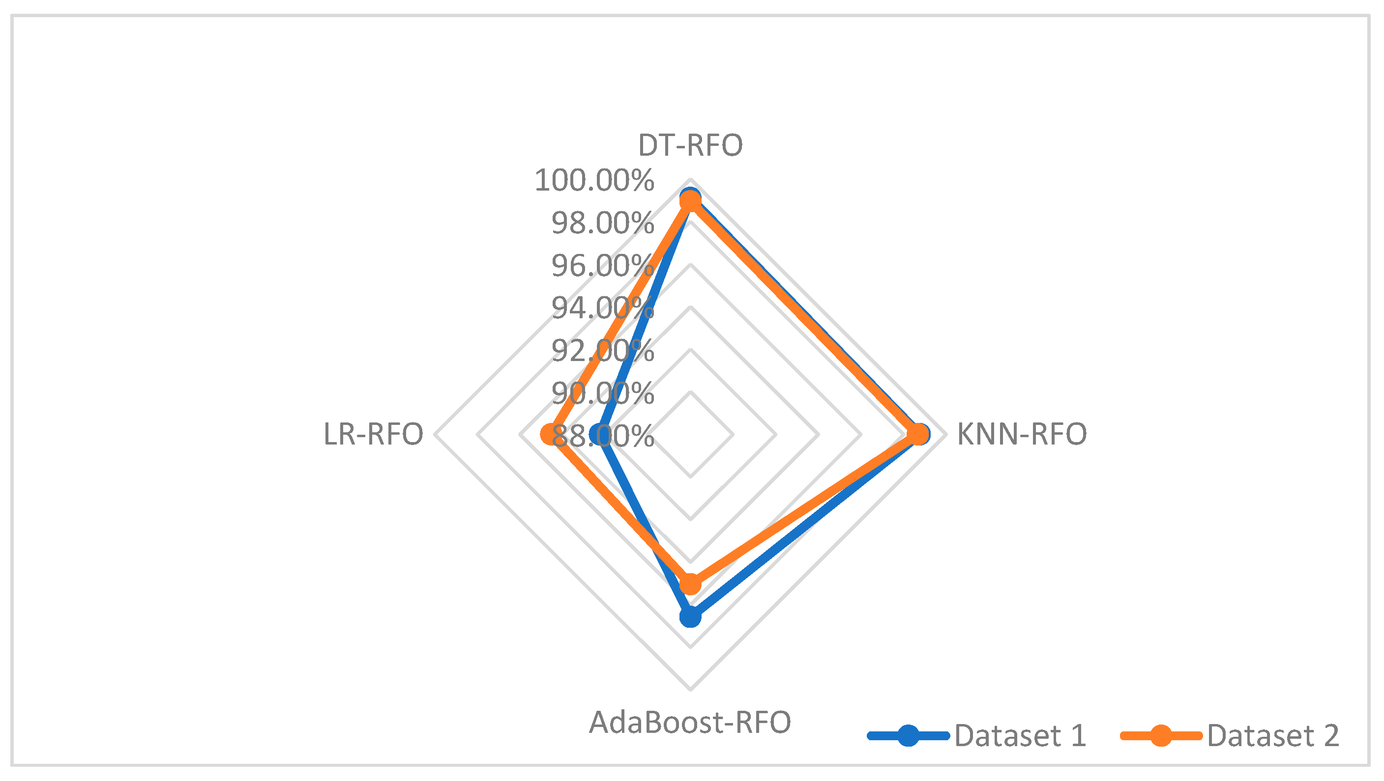
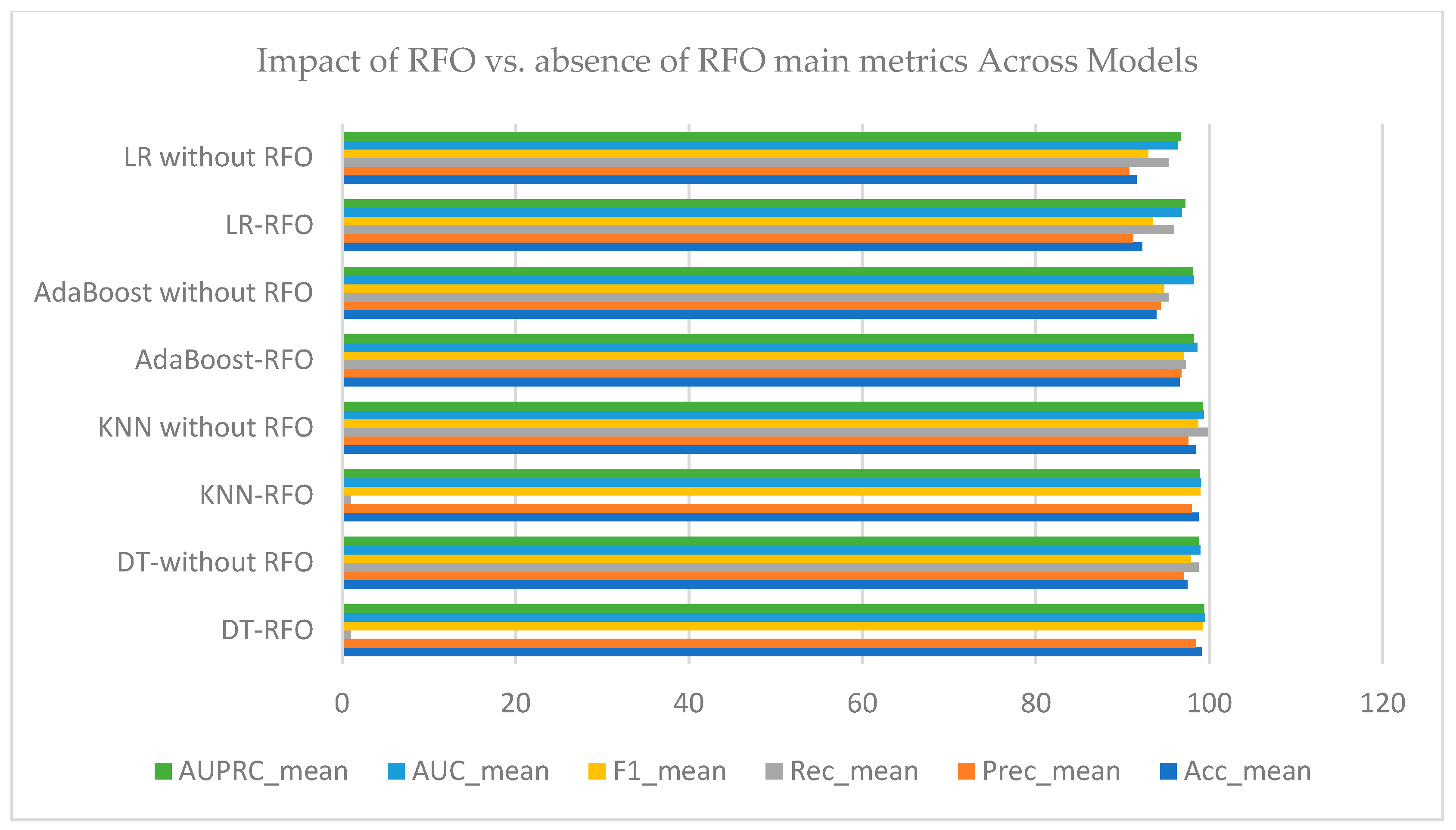
To confirm the generalizability of the suggested approach, a comparative evaluation was performed utilizing a new X spam dataset in conjunction with the original spam detection benchmark. After the preparation processes outlined in Section 4.2, a consistent subset of eleven out of eighteen features was retained, ensuring that both datasets could be compared fairly. The same four classifiers were used in the classification experiments. Figure 10. shows the accurate results. The results demonstrate that all models had almost flawless classification performance with respect to Dataset 1, which was quite similar to the results on the second dataset.

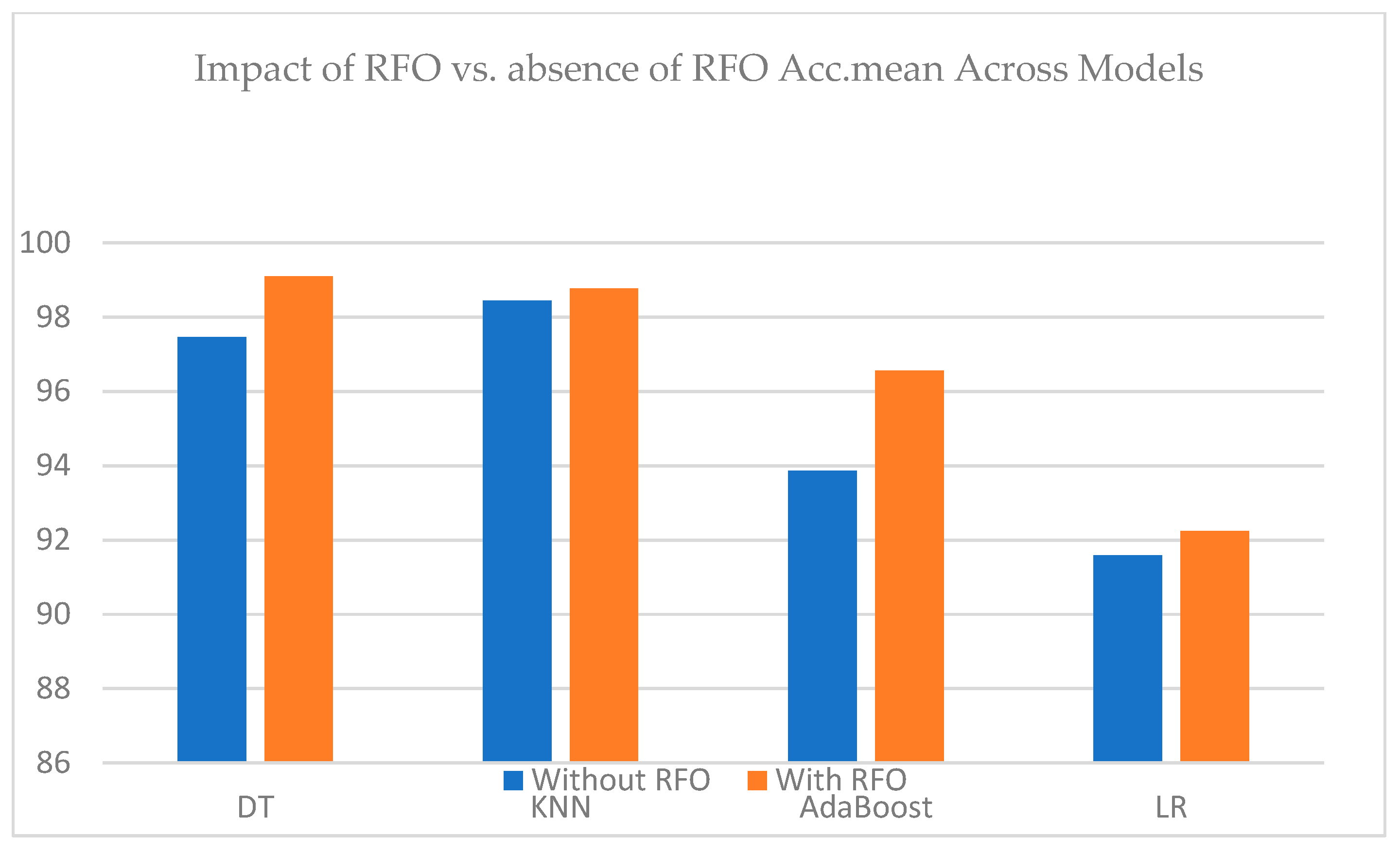
This consistency shows that the chosen characteristics can be used in many different scenarios and that the RFO pipeline can handle a wide range of spam classification. These findings, shown in Figure 11 and Figure 12, collectively indicate that lightweight, resilient XAI-powered machine learning provides a scalable and efficient solution for spam detection in many environments.

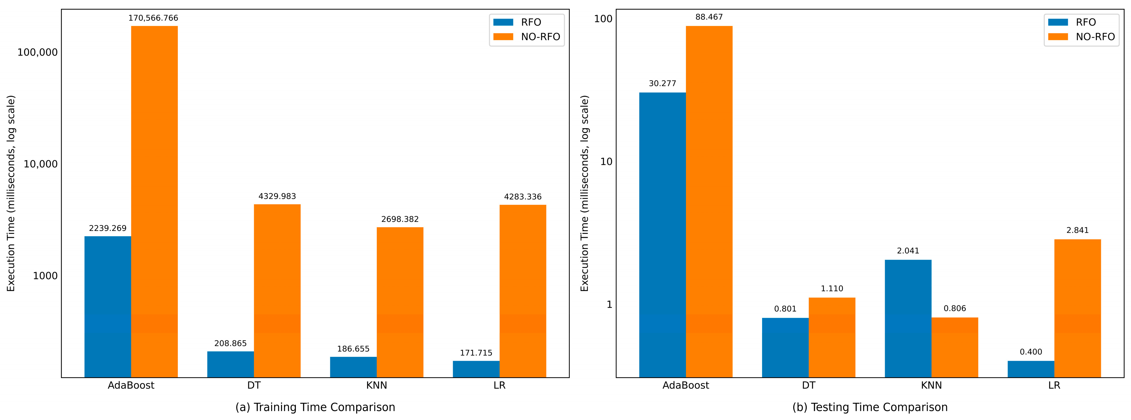
Figure 13 summarize execution times (log scale) for the four classifiers under the RFO and NO-RFO configurations. Training is markedly faster with RFO for all models—reductions are one to two orders of magnitude—while inference times remain comparable or slightly better with RFO (AdaBoost, DT, and LR). KNN exhibits a small inference advantage without RFO, consistent with its distance-based mechanics, but this does not offset the large training time gains observed elsewhere. Overall, RFO offers the best computational profile—substantially lower training costs with no meaningful degradation with respect to test times—and is therefore the preferred setting for our pipeline.

Table 8. Benchmarking our research in comparison with other studies.

Author	Dataset	Methodology	Performance Results (%)
[35]	X Dataset (by X API)	(IT2-M) (FIS) (IT2-S) (FIS) (IT1-M) (FIS) (IT1-S) (FIS)	Accuracy = 95.5 Precision = 95.7 Recall = 96.7 F1 score = 96.2 AUC = 97.1
[36]	SemCat-(2018)	TOBEAT leveraging BERT and CNN	Accuracy = 94.97 Precision = 94.05 Recall = 95.88 F1 score = 94.95
[37]	X Dataset (by hatebase.org)	A clustering framework using probabilistic rules and fuzzy sentiment classification	Accuracy = 94.53 Precision = 92.54 Recall = 91.74 F1 score = 92.56 AUC = 96.45
[47]	X Dataset (Sem-Eval-2014 and Bamman)	Classification methodology based on (FL)	Accuracy = 90.9 Precision = 95.7 Recall = 82.4 F1 score = 87.4
[48]	X Dataset (by [48])	Ensemble learning technique with random oversampling (ROS) plus random undersampling (RUS) and fuzzy-based oversampling (FOS)	Mean P = 0.76–0.78 Mean F = 0.76–0.55 Mean FP = 0.11 TP = 0.74–0.43
[39]	X Dataset (by X API)	(HMPS) Hierarchical meta-path-based approach with feedback and default one-class classifier	Precision = 95.0 Recall = 90.0 F1 score = 93.0 AUC = 92.0
[49]	X Dataset (by X API)	Deep learning (DL) methodology utilizing a multilayer perceptron (MLP) algorithm	Precision = 92.0 Recall = 88.0 F1 score = 89.0
[34]	X Dataset (by www.unipi.it)	Ensemble-based XGBoost with random forest	Accuracy = 90 Precision = 91.0 Recall = 86.0 F1 score = 89.0
[50]	X Dataset (HSpam14 and 1KS10KN)	Ensemble method utilizing convolutional neural network models and a feature-based model	Accuracy = 95.7 Precision = 92.2 Recall = 86.7 F1 score = 89.3
[51]	X Dataset (by [49])	LR, SVM, and RF utilizing various N-gram character features.	Precision = 79.5 Recall = 79.4 F1-score = 79.4
Proposed method	X Dataset 1 (by [35])	Nature-inspired method with an ensemble learning approach using 9 features	Accuracy DT-RFO = 99.10 KNN-RFO = 98.77 AdaBoost-RFO = 96.57 LR-RFO = 92.24
	X Dataset 2 (by [52])	Nature-inspired method with an ensemble learning approach using 11 features	Accuracy DT-RFO = 98.94 KNN-RFO = 98.67 AdaBoost-RFO = 95.04 LR-RFO = 94.52

presents an analytical comparison of related studies that employed an identical dataset, establishing a definitive standard for our method’s efficacy in comparison to other prominent techniques used in the field of X spam account detection. This contrast is essential for situating our method’s efficiency, specifically emphasizing the improvements attained within our amalgamation of XAI methods along with the ensemble model, a technique that is rarely used in other studies.

6. Conclusions

This study introduces a lightweight, robust XAI-powered ML method for X spam account detection. The proposed architecture consists of four components: data preprocessing, feature selection, spam classification, and explanation of model predictions. With respect to data preprocessing, the dataset is subsequently processed by RFO, which selects a subset of nine features from spam account datasets. Machine learning algorithms are trained and evaluated using the subset feature. The model’s prediction is ultimately interpreted via the application of Shapley values.

The abilities and shortcomings of the proposed model are put into perspective by comparisons. The proposed system yielded outstanding results and was empirically assessed using two datasets, achieving accuracies of 99.10%, 98.77%, 96.57%, and 92.24% using RFO with DT, KNN, AdaBoost, and LR, respectively, on Dataset 1. Values of 98.94%, 98.67%, 95.04%, and 94.52% were obtained in Dataset 2. Swarm and summary Shapley values were leveraged to clarify the decision-making processes, hence improving model interpretability. The results provide a clear technique that improves interpretation in complex environments, such as cybersecurity.

These results stress the pivotal importance of optimal feature subset selection and AI explainability, necessitating additional investigation into nature-inspired optimization algorithms and XAI methodologies.

However, the proposed approach has limitations. The efficacy of the proposed system is intricately linked to the spam account dataset’s characteristics. The estimations employed by SHAP underscore the intricate equilibrium between performance, explainability, and generalizability. The forthcoming work, motivated by our results, appears both motivated and essential. We intend to evaluate the versatility of the proposed approach across other OSN platforms. Furthermore, with the intention of rectifying this approach’s constraints, future studies will explore different feature selection methodologies and the efficacy of ensemble learning approaches to improve efficiency and explainability.

References

1. Jethava, G.; Rao, U.P. Exploring security and trust mechanisms in online social networks: An extensive review. Comput. Secur. 2024, 140, 103790. [Google Scholar] [CrossRef]
2. Nevado-Catalán, D.; Pastrana, S.; Vallina-Rodriguez, N.; Tapiador, J. An analysis of fake social media engagement services. Comput. Secur. 2023, 124, 103013. [Google Scholar] [CrossRef]
3. de Keulenaar, E.; Magalhães, J.C.; Ganesh, B. Modulating Moderation: A History of Objectionability in Twitter Moderation Practices. J. Commun. 2023, 73, 273–287. [Google Scholar] [CrossRef]
4. Murtfeldt, R.; Alterman, N.; Kahveci, I.; West, J.D. RIP Twitter API: A eulogy to its vast research contributions. arXiv 2024, arXiv:2404.07340. [Google Scholar] [CrossRef]
5. Song, J.; Lee, S.; Kim, J. Spam filtering in Twitter using sender-receiver relationship. In Recent Advances in Intrusion Detection: 14th International Symposium, RAID 2011, Menlo Park, CA, USA, 20–21 September 2011; Lecture Notes in Computer Science, Vol. 6961; Springer: Berlin/Heidelberg, Germany, 2011; pp. 301–317. [Google Scholar]
6. Delany, S.J.; Buckley, M.; Greene, D. SMS spam filtering: Methods and data. Expert Syst. Appl. 2012, 39, 9899–9908. [Google Scholar] [CrossRef]
7. Iman, Z.; Sanner, S.; Bouadjenek, M.R.; Xie, L. A longitudinal study of topic classification on Twitter. In Proceedings of the Eleventh International AAAI Conference on Web and Social Media (ICWSM 2017), Montréal, QC, Canada, 15–18 May 2017; AAAI Press: Palo Alto, CA, USA, 2017; Volume 11, pp. 552–555. [Google Scholar] [CrossRef]
8. Rashid, H.; Liaqat, H.B.; Sana, M.U.; Kiren, T.; Karamti, H.; Ashraf, I. Framework for detecting phishing crimes on Twitter using selective features and machine learning. Comput. Electr. Eng. 2025, 124, 110363. [Google Scholar] [CrossRef]
9. Ahmad, S.B.S.; Rafie, M.; Ghorabie, S.M. Spam detection on Twitter using a support vector machine and users’ features by identifying their interactions. Multimed. Tools Appl. 2021, 80, 11583–11605. [Google Scholar] [CrossRef]
10. Abkenar, S.B.; Mahdipour, E.; Jameii, S.M.; Kashani, M.H. A hybrid classification method for Twitter spam detection based on differential evolution and random forest. Concurr. Comput. Pract. Exp. 2021, 33, e6381. [Google Scholar] [CrossRef]
11. Galli, A.; La Gatta, V.; Moscato, V.; Postiglione, M.; Sperlì, G. Explainability in AI-based behavioral malware detection systems. Comput. Secur. 2024, 141, 103842. [Google Scholar] [CrossRef]
12. Le, T.-T.-H.; Kim, H.; Kang, H.; Kim, H. Classification and explanation for intrusion detection system based on ensemble trees and SHAP method. Sensors 2022, 22, 1154. [Google Scholar] [CrossRef]
13. Braik, M.; Al-Hiary, H. Rüppell’s fox optimizer: A novel meta-heuristic approach for solving global optimization problems. Clust. Comput. 2025, 28, 292. [Google Scholar] [CrossRef]
14. Kaczmarek-Majer, K.; Casalino, G.; Castellano, G.; Dominiak, M.; Hryniewicz, O.; Kamińska, O.; Vessio, G.; Díaz-Rodríguez, N. PLENARY: Explaining black-box models in natural language through fuzzy linguistic summaries. Inf. Sci. 2022, 614, 374–399. [Google Scholar] [CrossRef]
15. Paic, G.; Serkin, L. The impact of artificial intelligence: From cognitive costs to global inequality. Eur. Phys. J. Spec. Top. 2025, 234, 3045–3050. [Google Scholar] [CrossRef]
16. Abusitta, A.; Li, M.Q.; Fung, B.C. Survey on Explainable AI: Techniques, challenges and open issues. Expert Syst. Appl. 2024, 255, 124710. [Google Scholar] [CrossRef]
17. Borgonovo, E.; Plischke, E.; Rabitti, G. The many Shapley values for explainable artificial intelligence: A sensitivity analysis perspective. Eur. J. Oper. Res. 2024, 318, 911–926. [Google Scholar] [CrossRef]
18. Selvakumar, V.; Reddy, N.K.; Tulasi, R.S.V.; Kumar, K.R. Data-Driven Insights into Social Media Behavior Using Predictive Modeling. Procedia Comput. Sci. 2025, 252, 480–489. [Google Scholar] [CrossRef]
19. Mienye, I.D.; Jere, N. A survey of decision trees: Concepts, algorithms, and applications. IEEE Access 2024, 12, 86716–86727. [Google Scholar] [CrossRef]
20. Mohammed, S.; Al-Aaraji, N.; Al-Saleh, A. Knowledge Rules-Based Decision Tree Classifier Model for Effective Fake Accounts Detection in Social Networks. Int. J. Saf. Secur. Eng. 2024, 14, 1243–1251. [Google Scholar] [CrossRef]
21. Halder, R.K.; Uddin, M.N.; Uddin, M.A.; Aryal, S.; Khraisat, A. Enhancing K-nearest neighbor algorithm: A comprehensive review and performance analysis of modifications. J. Big Data 2024, 11, 113. [Google Scholar] [CrossRef]
22. Teke, M.; Etem, T. Cascading GLCM and T-SNE for detecting tumor on kidney CT images with lightweight machine learning design. Eur. Phys. J. Spec. Top. 2025, 234, 4619–4634. [Google Scholar] [CrossRef]
23. Ouyang, Q.; Tian, J.; Wei, J. E-mail Spam Classification using KNN and Naive Bayes. Highlights Sci. Eng. Technol. 2023, 38, 57–63. [Google Scholar] [CrossRef]
24. Bisong, E. Logistic regression. In Building Machine Learning and Deep Learning Models on Google Cloud Platform: A Comprehensive Guide for Beginners; Apress: Berkeley, CA, USA, 2019; pp. 243–250. [Google Scholar] [CrossRef]
25. Sarker, S.K.; Bhattacharjee, R.; Sufian, M.A.; Ahamed, M.S.; Talha, M.A.; Tasnim, F.; Islam, K.M.N.; Adrita, S.T. Email Spam Detection Using Logistic Regression and Explainable AI. In Proceedings of the 2025 International Conference on Electrical, Computer and Communication Engineering (ECCE), Chittagong, Bangladesh, 13–15 February 2025; IEEE: Piscataway, NJ, USA, 2025; pp. 1–6. [Google Scholar] [CrossRef]
26. Bharti, K.K.; Pandey, S. Fake account detection in twitter using logistic regression with particle swarm optimization. Soft Comput. 2021, 25, 11333–11345. [Google Scholar] [CrossRef]
27. Khan, A.A.; Chaudhari, O.; Chandra, R. A review of ensemble learning and data augmentation models for class imbalanced problems: Combination, implementation and evaluation. Expert Syst. Appl. 2024, 244, 122778. [Google Scholar] [CrossRef]
28. Mohammed, A.; Kora, R. A comprehensive review on ensemble deep learning: Opportunities and challenges. J. King Saud Univ.-Comput. Inf. Sci. 2023, 35, 757–774. [Google Scholar] [CrossRef]
29. Xing, H.-J.; Liu, W.-T.; Wang, X.-Z. Bounded exponential loss function based AdaBoost ensemble of OCSVMs. Pattern Recognit. 2024, 148, 110191. [Google Scholar] [CrossRef]
30. Ferrouhi, E.M.; Bouabdallaoui, I. A comparative study of ensemble learning algorithms for high-frequency trading. Sci. Afr. 2024, 24, e02161. [Google Scholar] [CrossRef]
31. Abkenar, S.B.; Kashani, M.H.; Akbari, M.; Mahdipour, E. Learning textual features for Twitter spam detection: A systematic literature review. Expert Syst. Appl. 2023, 228, 120366. [Google Scholar] [CrossRef]
32. Qazi, A.; Hasan, N.; Mao, R.; Abo, M.E.M.; Dey, S.K.; Hardaker, G. Machine Learning-Based Opinion Spam Detection: A Systematic Literature Review. IEEE Access 2024, 12, 143485–143499. [Google Scholar] [CrossRef]
33. Imam, N.H.; Vassilakis, V.G. A survey of attacks against twitter spam detectors in an adversarial environment. Robotics 2019, 8, 50. [Google Scholar] [CrossRef]
34. Alnagi, E.; Ahmad, A.; Al-Haija, Q.A.; Aref, A. Unmasking Fake Social Network Accounts with Explainable Intelligence. Int. J. Adv. Comput. Sci. Appl. 2024, 15, 1277–1283. [Google Scholar] [CrossRef]
35. Atacak, İ.; Çıtlak, O.; Doğru, İ.A. Application of interval type-2 fuzzy logic and type-1 fuzzy logic-based approaches to social networks for spam detection with combined feature capabilities. PeerJ Comput. Sci. 2023, 9, e1316. [Google Scholar] [CrossRef]
36. Ouni, S.; Fkih, F.; Omri, M.N. BERT-and CNN-based TOBEAT approach for unwelcome tweets detection. Soc. Netw. Anal. Min. 2022, 12, 144. [Google Scholar] [CrossRef]
37. Ayo, F.E.; Folorunso, O.; Ibharalu, F.T.; Osinuga, I.A.; Abayomi-Alli, A. A probabilistic clustering model for hate speech classification in twitter. Expert Syst. Appl. 2021, 173, 114762. [Google Scholar] [CrossRef]
38. Liu, S.; Wang, Y.; Chen, C.; Xiang, Y. An Ensemble Learning Approach for Addressing the Class Imbalance Problem in Twitter Spam Detection. In Information Security and Privacy; Liu, J., Steinfeld, R., Eds.; Lecture Notes in Computer Science; Springer: Cham, Switzerland, 2016; Volume 9722, pp. 215–228. [Google Scholar] [CrossRef]
39. Gupta, S.; Khattar, A.; Gogia, A.; Kumaraguru, P.; Chakraborty, T. Collective classification of spam campaigners on Twitter: A hierarchical meta-path based approach. In Proceedings of the 2018 World Wide Web Conference (WWW ’18), Lyon, France, 23–27 April 2018; International World Wide Web Conferences Steering Committee (IW3C2): Geneva, Switzerland, 2018; pp. 529–538. [Google Scholar] [CrossRef]
40. Manasa, P.; Malik, A.; Alqahtani, K.N.; Alomar, M.A.; Basingab, M.S.; Soni, M.; Rizwan, A.; Batra, I. Tweet spam detection using machine learning and swarm optimization techniques. IEEE Trans. Comput. Soc. Syst. 2024, 11, 4870–4877. [Google Scholar] [CrossRef]
41. Krithiga, R.; Ilavarasan, E. Hyperparameter tuning of AdaBoost algorithm for social spammer identification. Int. J. Pervasive Comput. Commun. 2021, 17, 462–482. [Google Scholar] [CrossRef]
42. Ghourabi, A.; Alohaly, M. Enhancing spam message classification and detection using transformer-based embedding and ensemble learning. Sensors 2023, 23, 3861. [Google Scholar] [CrossRef] [PubMed]
43. Kohavi, R. A study of cross-validation and bootstrap for accuracy estimation and model selection. In Proceedings of the Fourteenth International Joint Conference on Artificial Intelligence (IJCAI-95), Montréal, QC, Canada, 20–25 August 1995; Mellish, C.S., Ed.; Morgan Kaufmann: San Mateo, CA, USA, 1995; Volume 2, pp. 1137–1145. [Google Scholar]
44. Schapire, R.E. Explaining AdaBoost. In Empirical Inference: Festschrift in Honor of Vladimir N. Vapnik; Schölkopf, B., Luo, Z., Vovk, V., Eds.; Springer: Berlin/Heidelberg, Germany, 2013; pp. 37–52. [Google Scholar] [CrossRef]
45. Djuric, M.; Jovanovic, L.; Zivkovic, M.; Bacanin, N.; Antonijevic, M.; Sarac, M. The AdaBoost Approach Tuned by SNS Metaheuristics for Fraud Detection. In Proceedings of the International Conference on Paradigms of Computing, Communication and Data Sciences (PCCDS 2022), Jaipur, India, 5–7 July 2022; Yadav, R.P., Nanda, S.J., Rana, P.S., Lim, M.-H., Eds.; Algorithms for Intelligent Systems. Springer: Singapore, 2023; pp. 115–128. [Google Scholar]
46. Jáñez-Martino, F.; Alaiz-Rodríguez, R.; González-Castro, V.; Fidalgo, E.; Alegre, E. A review of spam email detection: Analysis of spammer strategies and the dataset shift problem. Artif. Intell. Rev. 2023, 56, 1145–1173. [Google Scholar] [CrossRef]
47. Meriem, A.B.; Hlaoua, L.; Romdhane, L.B. A fuzzy approach for sarcasm detection in social networks. Procedia Comput. Sci. 2021, 192, 602–611. [Google Scholar] [CrossRef]
48. Liu, S.; Wang, Y.; Zhang, J.; Chen, C.; Xiang, Y. Addressing the class imbalance problem in twitter spam detection using ensemble learning. Comput. Secur. 2017, 69, 35–49. [Google Scholar] [CrossRef]
49. Ameen, A.K.; Kaya, B. Spam detection in online social networks by deep learning. In Proceedings of the 2018 International Conference on Artificial Intelligence and Data Processing (IDAP), Malatya, Turkey, 28–30 September 2018; IEEE: Piscataway, NJ, USA, 2018; pp. 1–4. [Google Scholar] [CrossRef]
50. Madisetty, S.; Desarkar, M.S. A neural network-based ensemble approach for spam detection in Twitter. IEEE Trans. Comput. Soc. Syst. 2018, 5, 973–984. [Google Scholar] [CrossRef]
51. Ashour, M.; Salama, C.; El-Kharashi, M.W. Detecting spam tweets using character N-gram features. In Proceedings of the 2018 13th International Conference on Computer Engineering and Systems (ICCES), Cairo, Egypt, 18–19 December 2018; IEEE: Piscataway, NJ, USA, 2018; pp. 190–195. [Google Scholar] [CrossRef]
52. Genuine/Fake User Profile Dataset. Kaggle. Available online: https://www.kaggle.com/datasets/whoseaspects/genuinefake-user-profile-dataset (accessed on 23 September 2025).
Figure 1. Comparison of traditional learning models and the explainable artificial intelligence model.
Electronics 14 04153 g001
Figure 2. Explainable AI in social network security: AI-powered spam detection.
Electronics 14 04153 g002
Figure 3. The operational mechanism of SHAP.
Electronics 14 04153 g003
Figure 4. A proposed methodology of spam identification via social networks.
Electronics 14 04153 g004
Figure 5. Class distribution before vs. after SMOTE.
Electronics 14 04153 g005
Figure 6. Depiction of the ROC curve of spam classification classes utilizing nine features picked via an RFO approach.
Electronics 14 04153 g006
Figure 7. Contrast among pooled out-of-fold precision–recall (PR) confidence intervals (CI) performance for four RFO-optimized classifiers.
Electronics 14 04153 g007
Figure 8. Visual depiction of the confusion matrix produced for classification utilizing the RFO technique on nine chosen features.
Electronics 14 04153 g008
Figure 9. (a) Summary plot illustrating the contribution of each attribute to the identification of X account categories via XAI- DT-RFO. (b) Illustrates a swarm chart depicting the feature contributions to the detection of every class of X accounts, utilizing an explainable spam detection system based on DT-RFO.
Electronics 14 04153 g009aElectronics 14 04153 g009b
Figure 10. Performance comparison of RFO on Dataset 1 and Dataset 2.
Electronics 14 04153 g010
Figure 11. Impact of RFO vs. absence of RFO mean of Acc. across models.
Electronics 14 04153 g011
Figure 12. Comparison of performance metrics in an aggregated form for all models.
Electronics 14 04153 g012
Figure 13. (a) Training time comparison of AdaBoost, DT, KNN, and LR classifiers with and without RFO, presented on a logarithmic scale in seconds. (b) Testing time comparison of the same classifiers under the same conditions.
Electronics 14 04153 g013