MSRDSN: A Novel Deep Learning Model for Fault Diagnosis of High-Voltage Disconnectors

Abstract

The operational state of high-voltage disconnectors plays a critical role in ensuring the safety, stability, and power supply reliability of electrical systems. To enable accurate identification of the operational status of high-voltage disconnectors, this paper proposes a fault diagnosis method based on a Multi-Scale Residual Depthwise Separable Convolutional Neural Network (MSRDSN). First, wavelet transform is applied to vibration signals to perform multi-scale analysis and enhance detail resolution. Then, a novel network architecture, referred to as RDSN, is constructed to extract discriminative high-level features from vibration signals by integrating residual learning blocks and depthwise separable convolution blocks. Furthermore, a combined loss function is introduced to optimize the RDSN, which simultaneously maximizes inter-class distance, minimizes intra-class distance, and reduces feature redundancy. Experimental results show that the proposed method achieves a top accuracy of 99.44% on a balanced dataset, outperforming the sub-optimal approach by 1.11%. This study offers a novel and effective solution for fault diagnosis in high-voltage disconnectors.

1. Introduction

As critical components of electrical infrastructure, high-voltage disconnectors are widely deployed in power systems, with their operational status directly determining the safety, stability, and power supply reliability of the entire grid [1,2,3,4]. However, due to the lack of an outer shell and prolonged exposure to outdoor environments, the structure of high-voltage disconnectors is inevitably susceptible to erosion, leading to mechanical abnormalities. Statistics indicate that mechanical faults account for 70% of all failures in high-voltage disconnectors, representing the most prevalent type of fault [5,6,7]. These mechanical issues often stem from underlying defects, and if not diagnosed and addressed promptly, they can easily trigger more severe safety incidents [8,9,10,11,12]. Therefore, employing condition monitoring and fault diagnosis techniques to timely identify mechanical defects in high-voltage disconnectors is crucial for ensuring the secure operation of power systems.

To address this issue, common fault diagnosis methods can be categorized into expert system-based and data-driven approaches. Expert systems primarily rely on planned maintenance, which depends heavily on the experience of maintenance personnel and consumes significant human and material resources. In recent years, with the advancement of computer technology, data-driven fault diagnosis methods have become a prominent research direction [13,14]. Currently, data-driven fault diagnosis methods for disconnectors mainly involve two processes: feature extraction and fault identification. For feature extraction, researchers typically analyze signals such as the main shaft angle [15,16], motor current [17], vibration [18], and torque [19,20] during the switching operation. Different types of signals require distinct feature extraction methods. For time-domain signals with simple frequency components (e.g., torque or shaft angle signals), commonly extracted features include mean value, peak, kurtosis, and similarity. For signals with complex frequency components and strong nonlinear characteristics (e.g., vibration and current signals), techniques such as short-time Fourier transform, empirical mode decomposition, and wavelet packet transform are often employed to extract time-frequency features. Among these, vibration signals are highly sensitive and can be measured non-invasively, making them one of the most widely used feature signals for mechanical fault diagnosis in disconnectors.

Currently, in terms of fault identification, machine learning-based fault diagnosis methods have been widely applied [21,22]. Teng et al. [23] proposed a method using Histogram of Oriented Gradients and Support Vector Machine (SVM) to assess the condition of disconnectors by analyzing switching status angles. Zhao et al. [18] decomposed vibration signals through ensemble empirical mode decomposition and filtered features based on kurtosis criteria. To accurately diagnose heating faults in disconnectors, Gong et al. [24] employed natural language processing, knowledge graph technology, and machine learning algorithms to mine both structured and unstructured data. Incorporating structured data, they introduced the SVM model based on a focal loss function to identify heating faults. In summary, these shallow learning methods can effectively recognize faults with distinct characteristics. However, they still rely heavily on expert experience, exhibit limited self-learning capability, and are prone to issues such as underfitting.

In recent years, deep learning has effectively addressed these challenges with its powerful self-learning capabilities. Unlike traditional methods, it operates independently of expert experience and provides end-to-end automated solutions for fault diagnosis [25,26]. Zhang et al. [27] employed a fast neural network to extract features from vibration signals for disconnector fault identification. Huang et al. [28] proposed a method for disconnector condition assessment based on infrared and visible light images, enabling early fault detection through the analysis of on-site photographs. In summary, while these deep learning methods can effectively identify various disconnector states through self-learning, they still fail to address the issue of model accuracy degradation.

To address the aforementioned issues, we propose a novel fault diagnosis method for disconnectors based on a multi-scale residual depthwise separable convolutional neural network, denoted as MSRDSN. The main contributions are summarized as follows:

(1)

A novel network architecture integrating residual learning and depthwise separable convolution has been proposed, effectively addressing the issues of accuracy degradation and feature redundancy in deep networks.

(2)

A combined loss function has been designed to simultaneously maximize inter-class distance and minimize intra-class distance, significantly enhancing feature discriminability.

(3)

Extensive experiments demonstrate that the proposed method maintains superior diagnostic accuracy even with imbalanced and limited data, while exhibiting strong generalization capability under different operating conditions.

The remainder of this paper is organized as follows. Section 2 introduces the preliminaries. Section 3 describes the methodology based on MSRDSN. Section 4 presents the experiments and result analysis. Section 5 concludes the paper.

2. Preliminaries

2.1. Residual Learning

Theoretically, the more layers stacked in a deep neural network, the stronger its learning capacity becomes. However, as depth increases, accuracy tends to saturate and then degrade rapidly. Residual learning addresses this challenge. The structure of a residual learning block is illustrated in Figure 1.

A residual block consists of a direct mapping from input to output combined with a skip connection from the input, which can be defined as

$$h(x)=f(x)+x$$

(1)

where x represents the input to the residual block, h(x) denotes the output, and f(x) represents the residual mapping function to be learned. When the input x already contains sufficiently complete fault features, the residual mapping function f(x) ceases further learning, and the output of the residual block becomes h(x) = x. The entire residual block effectively acts as an identity mapping, altering both the forward and backward propagation mechanisms of the neural network, thereby preventing performance degradation in deep networks.

2.2. Depthwise Separable Convolution

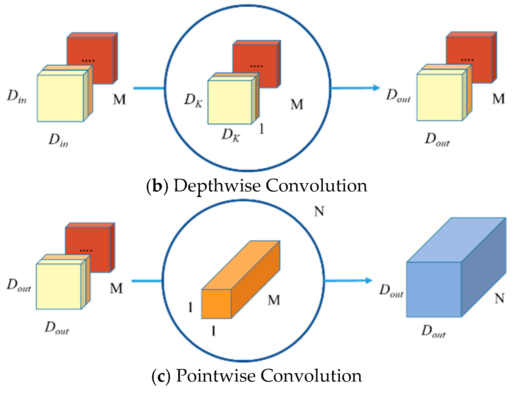
As shown in Figure 2, depthwise separable convolution (DSC) decomposes a standard convolution into two operations: a depthwise convolution (DW) and a pointwise convolution (PW). The DW applies a single convolutional filter per input channel to capture spatial correlations within features. The PW then performs a 1 × 1 convolution to linearly combine the feature maps generated by the DW.

Suppose the input feature map size is $D_{in}\ast D_{in}$, the number of channels is $M$, the convolution kernel size is $D_K\ast D_K$, the number of convolution kernels is $N$, and the output feature map size is $D_{out}\ast D_{out}$, then the standard convolution layer is computed as

$$D_K\ast D_K\ast M\ast N\ast D_{in}\ast D_{in}$$

(2)

The DW is computed as

$$D_K\ast D_K\ast D_{in}\ast D_{in}\ast M$$

(3)

The PW is computed as

$$D_F\ast D_F\ast M\ast N$$

(4)

The DSC is computed as

$$D_K\ast D_K\ast D_F\ast D_F\ast M+D_F\ast D_F\ast M\ast N$$

(5)

The ratio of DSC to standard convolution is computed as

$${\displaystyle \frac{D_K\ast D_K\ast D_F\ast D_F\ast M+D_F\ast D_F\ast M\ast N}{D_K\ast D_K\ast M\ast N\ast D_F\ast D_F}}={\displaystyle \frac{1}{N}}+{\displaystyle \frac{1}{D_K^2}}$$

(6)

where the number of convolution kernels $N$ is generally greater than 1, the convolution kernel size $D_K\ast D_K$ is usually $3\times 3$, $5\times 5$, $7\times 7$. In this article, we choose a convolution kernel size of $3\times 3$, and the value of Equation (6) can be calculated to be less than 1. It can be seen that the DSC is less computationally intensive than the standard convolution.

2.3. Working Principle of High-Voltage Disconnectors

The complete operational procedure of high-voltage disconnectors centers around three core scenarios: “power-off, maintenance, and power restoration”, which can be specifically divided into power-off operations and power-on operations.

The primary objective of a power-off operation is to safely isolate equipment scheduled for maintenance, ensuring its reliable disconnection from energized parts and creating a visible break. During this process, the circuit breaker in the relevant loop must first be opened and confirmed to be in the open position to interrupt load current. Only afterward can the disconnector be operated: first, the line-side disconnector is opened, followed by the bus-side disconnector. This sequence aims to confine potential accidents to the line side in case of operational errors, preventing impacts on the busbar. After the disconnector is opened, a clear air gap forms between its contacts, providing a visual indication of electrical isolation. Finally, the grounding switch must be closed to discharge residual charges on the line or equipment, prevent electric shock from induced voltages, and provide direct grounding protection for maintenance personnel. Throughout this process, electrical or mechanical interlocking devices between the disconnector, circuit breaker, and grounding switch are critical, as they effectively prevent erroneous operations such as switching the disconnector under load.

The goal of a power-on operation is to safely restore power supply, following a sequence exactly opposite to the power-off procedure. Before operation, it must be confirmed that no personnel are working on the circuit to be energized and that the equipment is in sound condition. First, the grounding switch should be opened to remove the safety grounding state of the equipment. Then, with the circuit breaker confirmed to remain open, the bus-side disconnector is closed first, followed by the line-side disconnector. This sequence similarly minimizes potential hazards in case of operational errors. When closing the disconnector, it is essential to ensure proper contact and full insertion between the moving and fixed contacts. The final step is to close the circuit breaker, which energizes the circuit under load and restores normal power supply. During the power-on process, interlocking devices are equally essential to guarantee the correct operational sequence, and after completion, both on-site and remote double verification must confirm that the position indicators of the disconnector and circuit breaker show proper closure with adequate contact depth.

3. Methodology

3.1. MSRDSN Fault Diagnosis Procedure

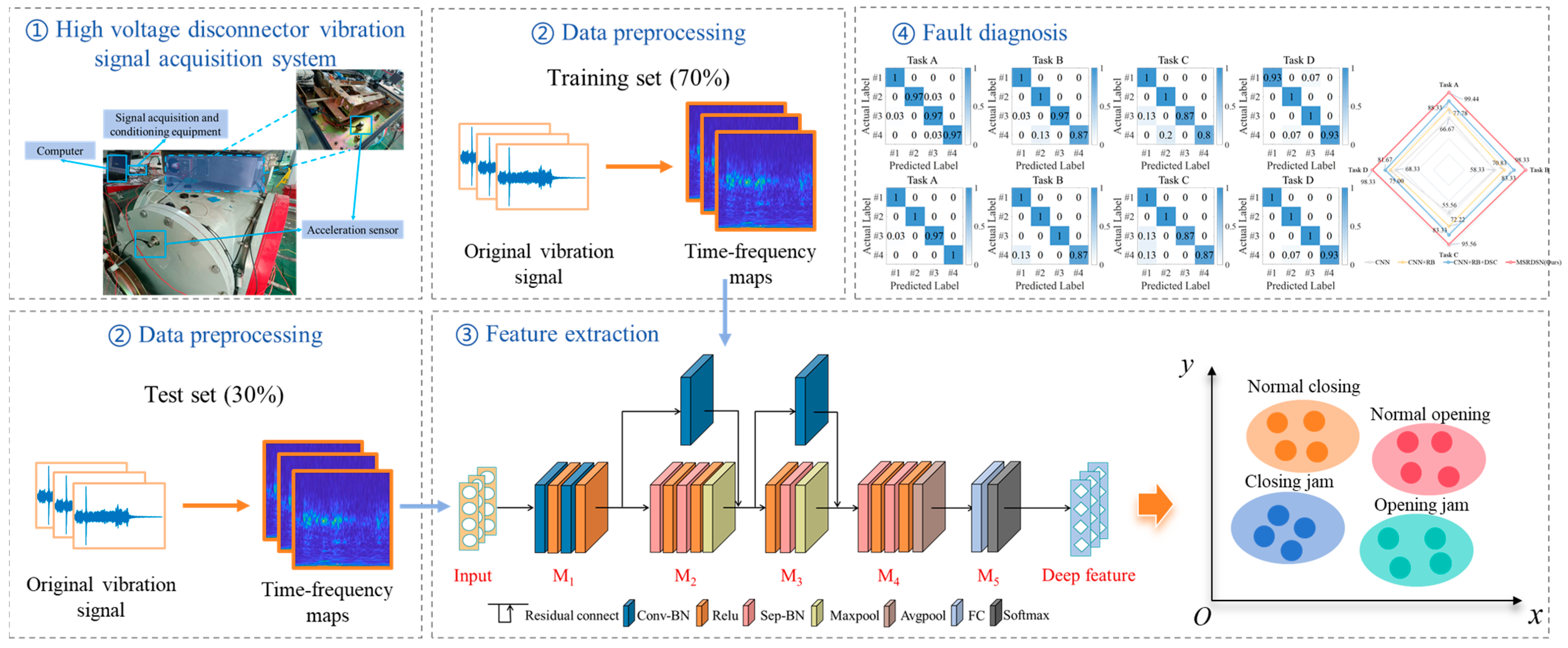
The fault diagnosis process based on the MSRDSN method is illustrated in Figure 3, which primarily includes three stages: fault signal preprocessing, feature extraction, and fault diagnosis. The detailed steps for each stage are as follows:

(1)

Fault Signal Preprocessing Stage: First, a vibration signal acquisition system for high-voltage disconnectors is established to collect vibration signals under different fault types. Next, all signal samples undergo wavelet transform to generate a dataset of two-dimensional time-frequency diagrams. Finally, the dataset is divided into training and testing sets in a 7:3 ratio.

(2)

Feature Extraction Stage: The two-dimensional time-frequency diagrams of the training set are input into the RDSN, and the parameters of each network layer are adjusted. The trained RDSN is then saved. Subsequently, the test set’s time-frequency diagrams are fed into the network, and downsampling is applied for dimensionality reduction to extract fault features from both the training and test sets. The effectiveness of feature extraction is validated using t-SNE for visualization.

(3)

Fault Diagnosis Stage: First, the test set data is input into the model for fault diagnosis. The predicted results are compared with the true labels to compute the confusion matrix and diagnostic accuracy. Finally, the diagnostic results are compared with those from other diagnostic algorithms.

3.2. Wavelet Transform

Wavelet transform offers unique advantages in analyzing vibration signals of disconnectors: its time-frequency localization capability enables effective capture of transient fault features in non-stationary signals, while its multi-scale analysis characteristic allows simultaneous retention of both high-frequency details and low-frequency contours. To further refine the disconnector signals, the wavelet transform method is employed to convert vibration signals into two-dimensional images. The mathematical expression for the continuous wavelet transform is given by:

$$\mathrm{WT}(a,b)=a^{-{\displaystyle \frac{1}{2}}}{\displaystyle {\int }_{-\infty }^{+\infty }f(t)\ast \psi (\frac{t-b}{a})}dt$$

(7)

$$\psi (t)=e^{-{\displaystyle \frac{t^2}{2}}}\cos (5t)$$

(8)

where $a>0$ is the scale parameter, b is the translation parameter, $\psi (t)$ is the mother wavelet function, and $f(t)$ is the vibration signal as a function of time t.

The effectiveness of wavelet transform hinges on the selection of a suitable mother wavelet function, which amplifies signal components that resemble the chosen wavelet while attenuating dissimilar ones. In the Morlet wavelet transform, the mother wavelet consists of a single-frequency complex sinusoidal function modulated by a Gaussian envelope, combined with a Gaussian function that exhibits exponential decay. These two components correspond to the time and frequency domains, respectively: the complex sinusoidal function captures oscillatory behavior in the frequency domain, while the Gaussian function provides finite support in the time domain. The mother wavelet function is mathematically defined as

$$\Phi (z)=e^{-{\displaystyle \frac{t^2}{2}}}{e}^{j{\omega }_{0}t}$$

(9)

By scaling and shifting the mother wavelet function, a series of wavelet functions can be derived as follows

$${\Phi }_{a,b}(z)={\displaystyle \frac{1}{\sqrt{a}}}{e}^{{\displaystyle \frac{-{(t-b)}^2}{2a^2}}}{e}^{{\displaystyle \frac{j{\omega }_0(t-b)}{a}}}$$

(10)

where a is the scale factor and b is the translation factor. By varying the value of a (scale transformation), the wavelet function is dilated or contracted. A larger a results in a lower center frequency of the function, slower exponential decay, a larger time-domain support interval, a narrower bandwidth in the frequency domain, and higher frequency resolution. Conversely, a smaller a produces the opposite effects. Due to its ability to provide richer information, the Morlet wavelet transform is selected for signal processing.

3.3. Feature Extraction

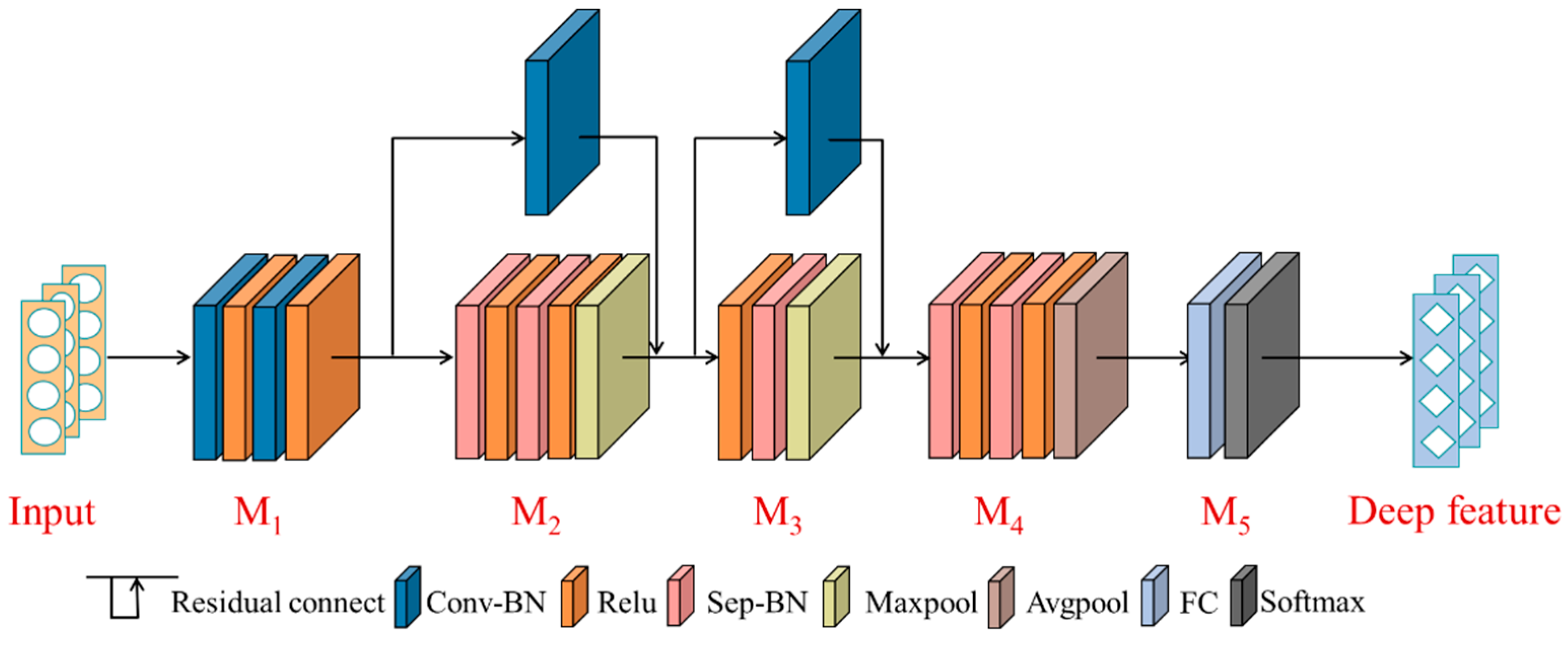
Deep neural networks possess the capability to extract abstract features from massive datasets. To fully leverage this feature extraction capacity while accelerating model convergence and mitigating network degradation, this paper proposes the RDSN model. The structure of the RDSN model, as illustrated in Figure 4, comprises two-dimensional convolutional layers, fully connected layers, downsampling layers, residual connections, and depthwise separable convolution layers.

The RDSN model takes three-channel time-frequency images as input. It continuously refines features through convolutional layers and depthwise separable convolutional layers, while incorporating residual connections to mitigate feature loss. The spatial dimensions are reduced via downsampling by setting strides in convolutional and pooling layers. Finally, a fully connected layer outputs one-dimensional features. The model employs Relu as the nonlinear activation function to accelerate training. To prevent vanishing gradient issues, batch normalization is applied to the results of each convolutional operation, ensuring a standard normal distribution and eliminating magnitude discrepancies between layers.

In experiments, the RDSN model operates in two phases: model training and feature extraction. During the training phase, the model is combined with a Softmax function. Training data passes through all model layers and the Softmax function via forward propagation to reach the class output layer. The output is then fed into the loss function for optimization.

The cross-entropy loss function serves as the objective function, enabling the trained deep network model to extract discriminative features. The cross-entropy loss function is expressed in Equation (11).

$$L_s=-{\displaystyle \sum _{i=1}^M{y}_i\log ({\widehat{y}}_i)}$$

(11)

where $y_i$ represents the true sample probability, ${\widehat{y}}_i$ denotes the predicted sample probability, and $M$ is the number of samples. However, the cross-entropy loss function does not account for the intra-class variability of faults. Samples within the same class may exhibit a scattered distribution or even overlap with other classes, leading to misclassification. The center loss is established based on the concept of clustering. During model training, it assigns a class center to each category (in the context of multi-class fault diagnosis, each class corresponds to a specific fault type). Feature vectors of the same fault type are encouraged to stay close to their class center while being pushed away from centers of other fault types. Assuming an input sample xi with a corresponding class label y_i, and the class center of y_i as c_yi, the center loss can be defined as

$$L_c={\displaystyle \frac{1}{2}}{\displaystyle \sum _{i=1}^n{‖x_i-c_{yi}‖}_2^2}$$

(12)

where n denotes the number of samples in a batch.

To address the limitation of the cross-entropy loss function in capturing intra-class fault variability and to enhance feature compactness, we train the RDSN using a combined loss function integrating both cross-entropy loss and center loss. This approach simultaneously increases inter-class distance between different fault types and reduces intra-class distance within the same fault type, thereby significantly improving the model’s discriminative power for fault categories. The combined loss function is defined as follows

$$Loss=L_s+\lambda L_c$$

(13)

where λ is used to control the weighting between the two losses. A smaller λ reduces the contribution of intra-class variance to the combined loss function, while a larger λ increases it.

During the feature extraction stage, the pre-trained RDSN model is employed to extract features from the entire dataset. This process yields low-dimensional feature vector representations of the data at the feature layer.

Overall, the RDSN model incorporates a lightweight network architecture that integrates depthwise separable convolutions, the Relu nonlinear activation function, and residual learning mechanisms. This design significantly reduces the number of parameters, accelerates convergence speed, shortens training time, preserves critical feature information, and reduces data dimensionality—thereby streamlining the subsequent fault diagnosis process.

3.4. Fault Diagnosis

In the fault diagnosis stage, the test set is input into the trained model. The predicted labels for the test samples are determined using Euclidean distance, and the accuracy is calculated by comparing these predictions with the ground truth labels.

4. Experiments and Result Analysis

4.1. Experimental Data

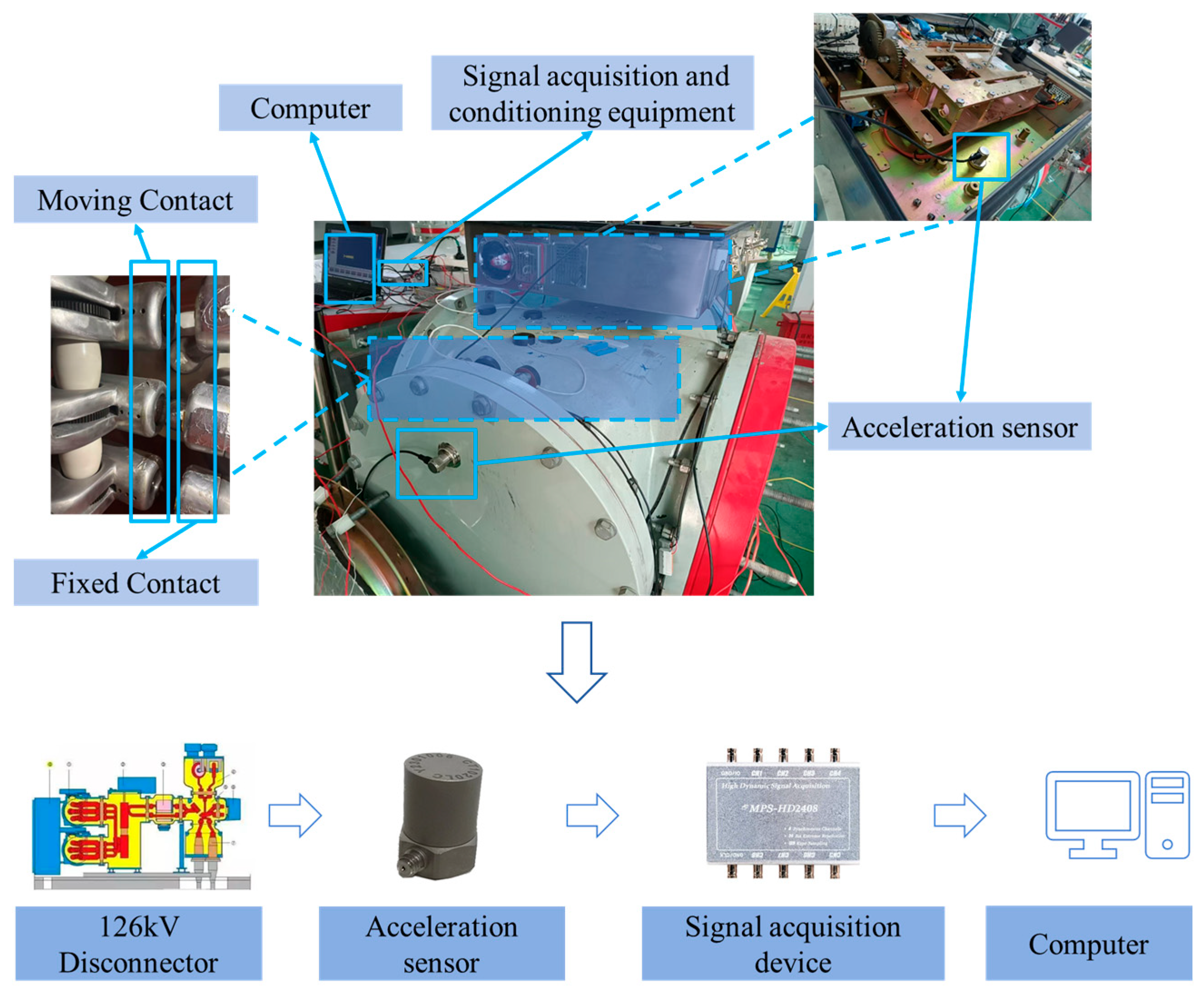
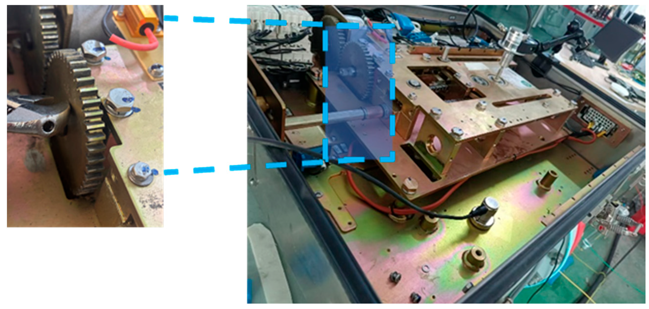
A specialized experimental platform for high-voltage disconnectors was constructed to perform data acquisition. As shown in Figure 5, the platform consists of a 126 kV high-voltage disconnector (model: ZF12B-126), a piezoelectric acceleration sensor, and a set of signal acquisition and conditioning equipment. The sensor (model: CT1020LC) has a measurement range of ±5 g, and the data acquisition device (model: HD2408) operates at a sampling frequency of 64 kHz. Using this platform, a dataset was constructed comprising four distinct states, with 150 samples per state, as detailed in

Table 1. Types of high-voltage disconnector fault data.

Label (No.)	Data Type
1	Normal closing
2	Normal opening
3	Closing jam
4	Opening jam

. The jamming fault setting is shown in Figure 6. The dataset was split into training and testing sets in a 7:3 ratio. Furthermore, to demonstrate the robustness of the proposed method on both balanced and imbalanced datasets, several diagnostic tasks were designed using the experimentally collected data, as summarized in

Table 2. Details of high-voltage disconnector data set settings.

Task (No.)	Samples
	Normal Closing	Normal Opening	Closing Jam	Opening Jam
A	150	150	150	150
B	150	100	100	50
C	100	100	50	50
D	50	50	50	50

.

4.2. Analysis of Results

4.2.1. Validity Analysis of RDSN

Following the model architecture described in Section 3.3, we refine the model hyperparameters through numerous trials, as detailed in

Table 3. Hyperparameters of the RDSN.

Module	Layer	Parameter
Module 1	(Conv-BN + Relu)-1 (Conv-BN + Relu)-2	Kernel size = 3 × 3 stride = 2 Kernel size = 3 × 3 stride = 1
Residual connection	Conv-BN	Kernel size = 1 × 1 stride = 2
Module 2	(Sep-BN + Relu) × 2 Maxpool	Kernel size = 3 × 3 stride = 1 Kernel size = 3 × 3 stride = 2
Residual connection	Conv-BN	Kernel size = 1 × 1 stride = 2
Module 3	Relu + Sep-BN Maxpool	Kernel size = 3 × 3 stride = 1 Pool size = 3 × 3 stride = 2
Module 4	(Sep-BN + Relu) × 2 Avgpool	Kernel size = 3 × 3 stride = 1 Pool size = 8 × 8 stride = 1
Module 5	FC + Softmax	Keep_prob = 0.5

. The multi-channel residual convolutional neural network is segmented into seven modules. The first module inputs a three-dimensional time-frequency map obtained from adaptive weighted fusion, measuring 64 × 64 × 3. The data then passes through modules 1 to 4 for progressive processing, ultimately producing a feature vector of 1 × 128. The number of convolutional kernels increases across the network to adequately map features, with each convolutional layer’s kernel count matching the output’s third dimension, thereby enhancing feature depth while reducing the image size.

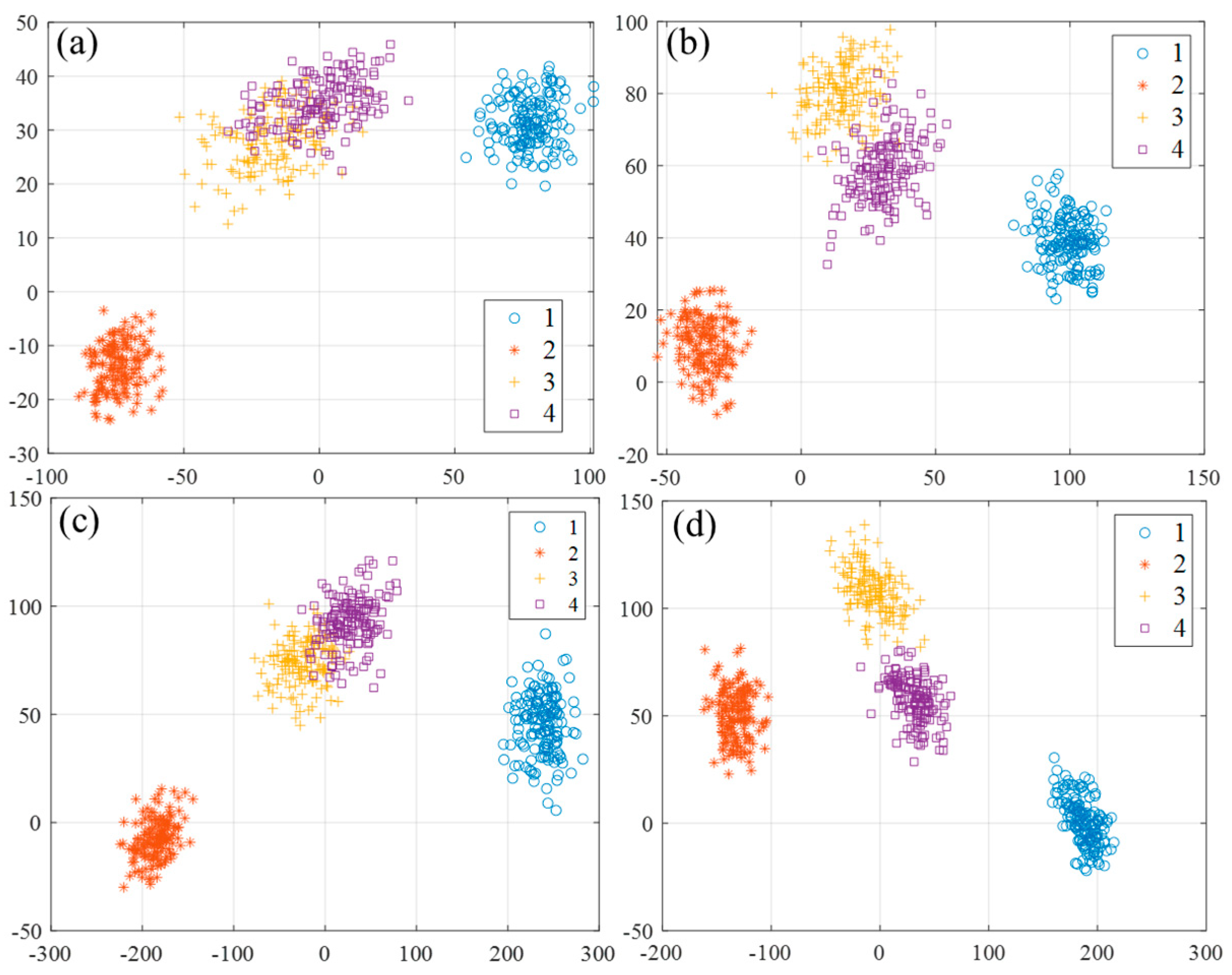
To validate the effectiveness of RDSN in feature extraction, we compared it with three widely used models in image recognition: AlexNet, GoogleNet, and ResNet50. t-SNE nonlinearly maps high-dimensional features into a two-dimensional space, where the coordinate axes are dimensionless and solely used to visualize similarity relationships between samples. The clustering degree of samples from the same category and the separation degree of samples from different categories reflect the quality of the feature representation. The results are shown in Figure 7. AlexNet and GoogleNet exhibited misclassification errors with unclear decision boundaries, indicating less effective feature extraction. ResNet50 showed partial confusion but relatively clearer decision boundaries, demonstrating improved feature extraction performance. In contrast, RDSN achieved distinct decision boundaries without any observable confusion, highlighting its superior feature extraction capability. These results confirm the exceptional ability of RDSN in both feature extraction and classification tasks.

4.2.2. Results and Comparative Analysis

To validate the effectiveness of the proposed method in diagnosing faults in high-voltage disconnectors, we compared it with several recently published fault diagnosis methods from the past five years, including MG-CL [29], Adaboost-SVM [30], CNN (D-S) [25], and AKNN-DMGCN [31]. Implementation details of these methods are provided in

Table 4. Comparison method implementation details.

Different Methods	Implementation Process
MG-CL [29]	First, the data augmentation module enhances the characteristics of the current signals. Then, the coarse-grained contrastive module performs preliminary fault diagnosis. Finally, the fine-grained contrastive module carries out detailed fault diagnosis.
Adaboost-SVM [30]	The process first conducts feature extraction on stator motor current signals and vibration signals using the envelope method and VMD. Then, it performs fault diagnosis through an Adaboost-optimized SVM.
CNN (D-S) [25]	The process first obtains two-dimensional features through wavelet packet transform and time-domain analysis. Then employs a CNN for fault diagnosis and finally enhances performance further with the support of D-S evidence theory.
AKNN-DMGCN [31]	First, a novel adaptive KNN graph construction method is proposed to build informative graphs. Subsequently, a Dynamic Multi-attention Graph Convolutional Network is applied for mechanical fault diagnosis.

, and comparative results are shown in

Table 5. Diagnostic effectiveness of different methods on different tasks (%).

Methods	Task A	Task B	Task C	Task D
MG-CL	96.67	90.83	87.78	86.67
Adaboost-SVM	96.11	92.50	88.89	85.00
AKNN-DMGCN	95.56	94.17	91.11	88.33
CNN (D-S)	98.33	97.50	94.44	96.67
MSRDSN(Ours)	99.44 (↑1.11)	98.33 (↑0.83)	95.56 (↑1.12)	98.33 (↑1.66)

. MG-CL utilizes two fault diagnosis modules for classification and effectively diagnoses disconnector faults, achieving an accuracy of 96.67% on Task A. Adaboost-SVM enhances diagnostic criteria through collaborative analysis of vibration and current signals, also achieving top performance on Task A. However, both machine learning methods exhibited a decline in accuracy under imbalanced sample conditions, due to their limited self-learning capability and inability to capture deeper features. AKNN-DMGCN constructs adaptive images and employs CNNs for fault diagnosis, but its performance drops significantly with reduced data volume due to high data dependency. In contrast, CNN (D-S) effectively extracts critical fault features and demonstrates robustness to both data imbalance and sample size reduction. The proposed MSRDSN method maintained high accuracy even when facing imbalanced and reduced sample sets, achieving superior performance across all four diagnostic tasks. This confirms its effectiveness in fault diagnosis for high-voltage disconnectors.

To further demonstrate the diagnostic performance of the proposed method, we compared it with the sub-optimal CNN (D-S) approach by plotting confusion matrices for both methods, as shown in Figure 8 and Figure 9.

From left to right, Figure 8 and Figure 9 display confusion matrices for different diagnostic tasks. The horizontal axis represents the predicted fault categories, while the vertical axis represents the true fault categories. The following observations can be made: (1) Under the condition of a sample size of 150, both methods exhibited excellent diagnostic performance. (2) When faced with imbalanced sample scenarios, CNN (D-S) experienced a more significant decline in accuracy and produced more misclassifications. (3) In cases of reduced sample sizes, the proposed method demonstrated superior adaptability. In summary, the proposed method achieved fewer misclassifications across all categories compared to CNN (D-S), highlighting its stronger fault identification capability and higher diagnostic accuracy.

4.2.3. Cross Validation

To validate the model’s effectiveness, we performed K-fold cross-validation (with K = 5) on Task A. The 150 samples of each state were evenly divided into 5 folds, with each fold containing 30 samples. A total of five validation experiments were conducted, each time selecting one fold as the test set. The results of the five experiments are shown in

Table 6. 5-fold cross-validation results.

K-Fold	Accuracy (%)
1	96.67
2	93.33
3	100.00
4	96.67
5	96.67
Average	96.67

. The model achieved accuracy rates of 96.67%, 93.33%, 100.00%, 96.67%, and 96.67% in the five validations, with an average accuracy of 96.67% and a standard deviation of 2.36%, demonstrating the model’s stability.

4.2.4. Multi-Indicator Performance Evaluation

To comprehensively evaluate the performance of the proposed model, we calculated several key evaluation metrics: recall rate and F1-score. These metrics are crucial for assessing the accuracy and reliability of the diagnostic model in identifying faults.

Table 7. Performance evaluation results.

Task	Recall (%)	F1 (%)
A	96.67	98.34
B	91.67	94.88
C	94.44	95.00
D	96.67	97.49

presents the performance evaluation results of MSRDSN across different tasks, including a detailed comparison of recall rates and F1-scores.

The proposed model demonstrates excellent and stable comprehensive performance across all four diagnostic tasks. Specifically, the recall rates all exceed 91.67% (reaching up to 96.67%), indicating the model’s strong capability in detecting true faults and effectively avoiding missed detections. Meanwhile, the F1-scores all surpass 94.88% (reaching up to 98.34%), reflecting an outstanding balance between fault identification sensitivity and false alarm control while maintaining high precision. Although Task B shows relatively lower performance metrics, the minimal performance fluctuations across all tasks (with standard deviations of approximately 2.18% for recall rate and 1.73% for F1-score) further validate the model’s powerful generalization capability and robustness, fully demonstrating its high reliability for practical engineering applications.

4.2.5. Ablation Experiments

Our proposed model is built upon a baseline model (CNN with cross-entropy loss function). By incorporating residual connections, depthwise separable convolutional blocks, and a combined loss function, we enhanced this baseline architecture. To evaluate the contribution of each component to the overall model performance, we conducted a series of ablation studies.

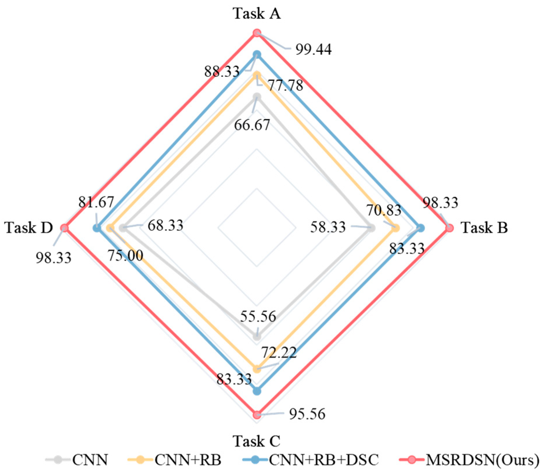
The specific results are shown in Figure 10. In Task D, the baseline model achieved a maximum accuracy of 68.33%. In the second experimental group, we added residual connections to the baseline model, which alleviated network degradation. This modification also improved accuracy by 11.11% in Task A. In the third experimental group, we further incorporated depthwise separable convolutions to refine the model. This effectively reduced computational complexity while enriching the model’s receptive field. The final experimental group represents our proposed model, which replaces the cross-entropy loss function with a combined loss function. This achieved minimized intra-class distance, maximized inter-class distance, and reduced redundancy.

The above ablation experiments demonstrate that each module of the proposed method is indispensable. These results validate the effectiveness of our approach for fault diagnosis in high-voltage disconnectors.

4.2.6. Parameter Analysis

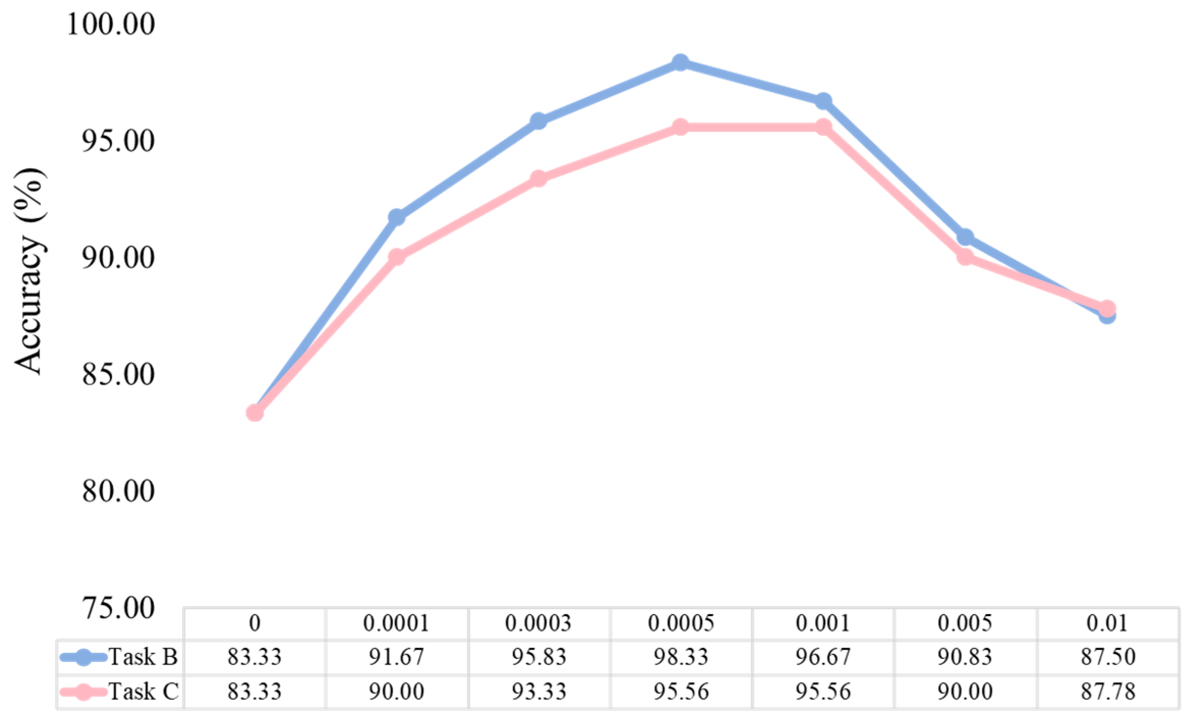
We further investigated the impact of different hyperparameter λ values in the combined loss function on model performance. The classification results for Tasks B and C are shown in Figure 11. When λ = 0, the classification accuracy for both tasks was 83.33%. This occurs because the center loss becomes inactive, leaving the cross-entropy loss function to act alone, which fails to account for intra-class variability among categories. As λ increases within the range of 0.0003 to 0.001, the model accuracy improves. The optimal accuracy for both tasks is achieved at λ = 0.0005. However, when λ increases to 0.005 or 0.01, the accuracy declines. This is because the optimization objective of the combined loss function becomes overly biased toward minimizing intra-class distance, deviating from the goal of maximizing inter-class distance.

4.2.7. Universal Analysis

The method proposed in this paper primarily consists of a residual structure, multi-scale wavelet transform, depthwise separable convolution architecture, and a combined loss function. It fundamentally addresses common challenges in vibration signal feature extraction and pattern recognition. This methodological framework can be extended to mechanical fault diagnosis of other electrical equipment such as circuit breakers and transformers. To adapt the method to different equipment characteristics, the following adjustments can be implemented: (1) Optimize the scale parameters of the wavelet transform based on the vibration characteristics of the target equipment. (2) Adjust the dimensionality of the network’s output layer according to the number of fault types. (3) Retrain the model using operational data specific to the target equipment.

5. Conclusions

To address the fault diagnosis problem in high-voltage disconnectors, this paper proposes a fault diagnosis method based on a residual depthwise separable network and center loss optimization. Compared to existing feature extraction models, the proposed RDSN extracts more discriminative features. By incorporating center loss into the cross-entropy loss, a combined loss function is established, which reduces intra-class distance while increasing inter-class variability, effectively improving the model’s fault diagnosis accuracy. Furthermore, different diagnostic tasks were designed to validate the method under various operating conditions of disconnectors. The results demonstrate that the proposed method achieves excellent performance in diagnosing faults in high-voltage disconnectors under diverse working conditions. In future work, we will explore simulating more types of mechanical faults in laboratory environments to further enhance the model’s generalization capability.

References

1. Zhang, Z.; Hao, Y.; Peng, J.; Yang, L.; Gao, C.; Wang, G.; Zhou, F.; Yang, Y.; Cao, H.; Li, L. A three-factor accelerated aging test platform of thermal, mechanical compression, pressured sf 6, and a leakage test system for GIS O-RING seals. IEEE Trans. Instrum. Meas. 2021, 70, 7501511. [Google Scholar]
2. Han, X.; Li, J.; Zhang, L.; Pang, P.; Shen, S. A novel pd detection technique for use in GIS based on a combination of uhf and optical sensors. IEEE Trans. Instrum. Meas. 2018, 68, 2890–2897. [Google Scholar] [CrossRef]
3. Xu, H.; Meng, C.; Huang, Q.; Luo, C.; Zhang, J.; Liu, Z. Time-frequency vibration characteristics analysis of disconnectors of GIS equipment with poor contact mechanical defect. In Proceedings of the 2021 IEEE 5th International Conference on Condition Assessment Techniques in Electrical Systems (CATCON), Kozhikode, India, 3–5 December 2021; IEEE: New York, NY, USA, 2021; pp. 215–219. [Google Scholar]
4. Schichler, U.; Koltunowicz, W.; Endo, F.; Feser, K.; Giboulet, A.; Girodet, A.; Hama, H.; Hampton, B.; Kranz, H.G.; Lopez-Roldan, J. Risk assessment on defects in GIS based on pd diagnostics. IEEE Trans. Dielectr. Electr. Insul. 2013, 20, 2165–2172. [Google Scholar] [CrossRef]
5. Carvalho, A.; Cormenzana, M.L.; Furuta, H.; Grieshaber, W.; Hyrczak, A.; Kopejtkova, D.; Krone, J.G.; Kudoke, M.; Makareinis, D.; Martins, J.F. Final Report of the 2004–2007 International Enquiry on Reliability of High Voltage Equipment, Part 1-Summary and General Matters; CigrÉ technical brochure no. 509; CIGRÉ: Paris, France, 2012. [Google Scholar]
6. Carvalho, A.; Cormenzana, M.L.; Furuta, H.; Grieshaber, W.; Hyrczak, A.; Kopejtkova, D.; Krone, J.G.; Kudoke, M.; Makareinis, D.; Martins, J.F. Final Report of the 2004–2007 International Enquiry on Reliability of High Voltage Equipment, Part 3-Disconnectors and Earthing Switches; CIGRÉ Technical Brochure No. 511; CIGRÉ: Paris, France, 2012. [Google Scholar]
7. Carvalho, A.; Cormenzana, M.L.; Furuta, H.; Grieshaber, W.; Hyrczak, A.; Kopejtkova, D.; Krone, J.G.; Kudoke, M.; Makareinis, D.; Martins, J.F. Final Report of the 2004–2007 International Enquiry on Reliability of High Voltage Equipment, Part 4-Instrument Transformers; CIGRÉ Technical Brochure No. 512; CIGRÉ: Paris, France, 2012. [Google Scholar]
8. Zhong, Y.; Hao, J.; Liao, R.; Wang, X.; Jiang, X.; Wang, F. Mechanical defect identification for gas-insulated switchgear equipment based on time-frequency vibration signal analysis. High Volt. 2021, 6, 531–542. [Google Scholar] [CrossRef]
9. Zhong, Y.; Hao, J.; Ding, Y.; Liao, R.; Xu, H.; Li, X. Novel GIS mechanical defect simulation and detection method based on large current excitation with variable frequency. IEEE Trans. Instrum. Meas. 2022, 71, 3519815. [Google Scholar] [CrossRef]
10. Feng, J.; Sun, L.; Chen, W.; Su, Y.; Shu, Y.; Zhao, L. Vibration characteristics of GIS isolating switch under different operating conditions. High Volt. Eng. 2021, 47, 4314–4322. [Google Scholar]
11. Li, K.; Chen, F.; Yang, H.; Yuan, H.; Yang, A.; Wang, X.; Rong, M. Intelligent diagnosis for mechanical faults of high voltage disconnector based on attitude sensor. Power Syst. Technol. 2023, 47, 3781–3790. [Google Scholar]
12. Xu, S.; Yu, H.; Wang, H.; Chai, H.; Ma, M.; Chen, H.; Zheng, W. Simultaneous diagnosis of open-switch and current sensor faults of inverters in IM drives through reduced-order interval observer. IEEE Trans. Ind. Electron. 2025, 72, 6485–6496. [Google Scholar] [CrossRef]
13. Xu, S.; Liu, J.; Li, K.; Fu, S. Research on feature extraction and condition identification method for transformer vibration signals based on GWO-VMD and SOM neural network. Power Syst. Big Data 2025, 28, 30–40. [Google Scholar]
14. Zhang, F.; Wan, A. Fault diagnosis of planetary gearbox of wind turbine based on double attention mechanism and transfer learning. Power Syst. Big Data 2024, 27, 1–9. [Google Scholar]
15. Qiu, Z.; Ruan, J.; Huang, D. Mechanical fault diagnosis of outdoor high-voltage disconnector. IEEJ Trans. Electr. Electron. Eng. 2016, 11, 556–563. [Google Scholar] [CrossRef]
16. Liu, K. Mechanical fault diagnosis of high voltage disconnector based on intelligent live test technology. In Proceedings of the IEEE 3rd International Conference Electron Device Mechanical Engineering, Suzhou, China, 3 May 2020; IEEE: New York, NY, USA, 2020; pp. 138–140. [Google Scholar]
17. Shi, K.; Lin, X.; Xu, J. Design of permanent magnet motor actuator used in 550 kV gas-insulated switchgear disconnector. Adv. Mech. Eng. 2015, 7, 1687814015575428. [Google Scholar] [CrossRef]
18. Zhao, L.; Hong, G.; Wang, Z.; Chen, W.; Long, W.; Ren, J.; Wang, Z.; Huang, X. Research on fault vibration signal features of GIS disconnector based on EEMD and kurtosis criterion. IEEJ Trans. Electr. Electron. Eng. 2021, 16, 677–686. [Google Scholar] [CrossRef]
19. Zhou, T.; Ruan, J.; Yang, Z.; Liu, Y. Mechanical defect detection of porcelain column high-voltage disconnector based on operating torque. Int. J. Adv. Robot. Syst. 2020, 17, 1729881419900845. [Google Scholar] [CrossRef]
20. Zhou, T.; Ruan, J.; Liu, Y.; Peng, S.; Wang, B. Defect diagnosis of disconnector based on wireless communication and support vector machine. IEEE Access 2020, 8, 30198–30209. [Google Scholar] [CrossRef]
21. Yang, C.; Wu, X.; Gong, W.; Wang, Q.; Li, L. An intelligent identification algorithm for obtaining the state of power equipment in SIFT-based environments. Int. J. Perform. Eng. 2019, 15, 2382–2391. [Google Scholar] [CrossRef]
22. Zhao, W.; Wen, F.; Wu, S.; Chu, Z.; Sheng, Z.; Ji, K. Fault diagnosis of GIS disconnector based on BP neural network. In Proceedings of the 2021 13th International Symposium on Linear Drives for Industry Applications, Wuhan, China, 1–3 July 2021; IEEE: New York, NY, USA, 2021; pp. 1–5. [Google Scholar]
23. Teng, Y.; Tan, T.; Lei, C.; Yang, J.; Ma, Y.; Zhao, K.; Jia, Y.; Liu, Y. A novel method to recognize the state of high-voltage isolating switch. IEEE Trans. Power Deliv. 2019, 34, 1350–1356. [Google Scholar] [CrossRef]
24. Gong, Z.; Cao, Z.; Zhou, S.; Yang, F.; Shuai, C.; Ouyang, X.; Luo, Z. Thermal fault detection of high-voltage isolating switches based on hybrid data and BERT. Arab. J. Sci. Eng. 2024, 49, 6429–6443. [Google Scholar] [CrossRef]
25. Wang, Q.; Zhang, K.; Lin, S. Fault diagnosis method of disconnector based on CNN and D-S evidence theory. IEEE Trans. Ind. Appl. 2023, 59, 5691–5704. [Google Scholar] [CrossRef]
26. Chi, Y.; Jiao, Z.; Ji, H.; Wang, Q.; Ge, H.; Chi, F. Comparative study on substation isolating switch state recognition algorithms based on image similarity and deep learning. Power Syst. Big Data 2023, 26, 1–10. [Google Scholar]
27. Zhang, K.; Zhang, Y.; Wu, J.; Li, Z. Quick identification of open/closed state of GIS switch based on vibration detection and deep learning. Electronics 2023, 12, 3204. [Google Scholar] [CrossRef]
28. Huang, S.; Shang, B.; Song, Y.; Zhang, N.; Wang, S.; Ning, S. Research on Real-Time Disconnector State Evaluation Method Based on Multi-Source Images. IEEE Trans. Instrum. Meas. 2021, 71, 3505415. [Google Scholar] [CrossRef]
29. Xie, Q.; Tang, H.; Liu, B.; Li, H.; Wang, Z.; Dang, J. Disconnector fault diagnosis based on multi-granularity contrast learning. Processes 2023, 11, 2981. [Google Scholar] [CrossRef]
30. Zhang, Z.; Liu, C.; Wang, R.; Li, J.; Xiahou, D.; Liu, Q.; Cao, S.; Zhou, S. Mechanical fault diagnosis of a disconnector operating mechanism based on vibration and the motor current. Energies 2022, 15, 5194. [Google Scholar] [CrossRef]
31. Sui, G.; Yan, J.; Wu, Y.; Xu, Z.; Qi, M.; Zhang, Z. Mechanical fault diagnosis of high-voltage circuit breakers with dynamic multi-attention graph convolutional networks based on adaptive graph construction. Appl. Sci. 2024, 14, 4036. [Google Scholar] [CrossRef]
Figure 1. Residual learning block.
Electronics 14 04151 g001
Figure 2. The standard convolution in (a) are replaced by two layers: depthwise convolution in (b) and pointwise convolution in (c) to build a depthwise separable convolution.
Electronics 14 04151 g002aElectronics 14 04151 g002b
Figure 3. Fault diagnosis procedure of MSRDSN.
Electronics 14 04151 g003
Figure 4. Structure of the RDSN model.
Electronics 14 04151 g004
Figure 5. 126 kV disconnector experimental platform.
Electronics 14 04151 g005
Figure 6. Jamming fault setup.
Electronics 14 04151 g006
Figure 7. Feature extraction performance visualized by t-SNE for different models: (a) AlexNet, (b) GoogleNet, (c) ResNet50, (d) RDSN.
Electronics 14 04151 g007
Figure 8. Confusion matrix of CNN (D-S) on four tasks.
Electronics 14 04151 g008
Figure 9. Confusion matrix of the proposed MSRDSN on four tasks.
Electronics 14 04151 g009
Figure 10. Results of the ablation experiment showing the contribution of each module to model performance improvement.
Electronics 14 04151 g010
Figure 11. Effect of different λ on model accuracy.
Electronics 14 04151 g011