Article

EDAT-BBH: An Energy-Modulated Transformer with Dual-Energy Attention Masks for Binary Black Hole Signal Classification

by
Osman Tayfun Bişkin
Department of Electrical and Electronics Engineering, Burdur Mehmet Akif Ersoy University, Burdur 15030, Türkiye
Electronics 2025, 14(20), 4098; https://doi.org/10.3390/electronics14204098
Submission received: 6 August 2025 / Revised: 27 September 2025 / Accepted: 15 October 2025 / Published: 19 October 2025

Abstract

Gravitational-wave (GW) detection has become a significant area of research following the first successful observation by the Laser Interferometer Gravitational-Wave Observatory (LIGO). The detection of signals emerging from binary black hole (BBH) mergers have challenges due to the presence of non-Gaussian and non-stationary noise in observational data. Using traditional matched filtering techniques to detect BBH merging are computationally expensive and may not generalize well to unexpected GW events. As a result, deep learning-based methods have emerged as powerful alternatives for robust GW signal detection. In this study, we propose a novel Transformer-based architecture that introduces energy-aware modulation into the attention mechanism through dual-energy attention masks. In the proposed framework, Q-transform and discrete wavelet transform (DWT) are employed to extract time–frequency energy representations from gravitational-wave signals which are fused into energy masks that dynamically guide the Transformer encoder. In parallel, the raw one-dimensional signal is used directly as input and segmented into temporal patches, which enables the model to leverage both learned representations and physically grounded priors. This proposed architecture allows the model to focus on energy-rich and informative regions of the signal in order to enhance the robustness of the model under realistic noise conditions. Experimental results on BBH datasets embedded in real LIGO noise show that EDAT-BBH outperforms CNN-based and standard Transformer-based approaches, achieving an accuracy of 0.9953, a recall of 0.9950, an F1-score of 0.9953, and an AUC of 0.9999. These findings demonstrate the effectiveness of energy-modulated attention in improving both the interpretability and performance of deep learning models for gravitational-wave signal classification.

1. Introduction

Gravitational waves (GWs) were introduced by Albert Einstein within the framework of the general theory of relativity [1]. He theorized that the gravitational waves are disturbances in space–time produced by the motion of extremely massive and accelerating objects such as black holes or neutron stars. These waves often originate from dynamic cosmic processes like collisions or explosions. The first successful observation of such waves was associated with the GW150914 event, officially reported in September 2015 by the Laser Interferometer Gravitational-Wave Observatory (LIGO) collaboration [2]. The analysis revealed that the waves originated from the merger of two black holes approximately 1.3 billion light-years away.
One of the systems that generates GWs is binary black holes (BBHs) and the study of BBHs is interesting and important for gravitational-wave research. These cosmic systems emit gravitational waves that offer critical information about their properties, origins, and development. However, identifying these signals has a considerable challenge due to their weakness compared to the dominant background noise caused by instrumental and environmental noise [3,4,5]. In order to overcome this issue, scientists employed advanced analytical techniques such as matched filtering and template matching, which help to detect the weak signals within the data from gravitational-wave observatories [6,7]. However, noises are non-Gaussian and non-stationary signals and these techniques are not always a good method because of including high computational cost and unexpected GW events [8]. Therefore, machine learning and deep learning techniques become an alternative solution for detection of gravitational waves. In [6,9], the researchers highlighted the efficiency of deep filtering methods that extend the range of detectable gravitational-wave signals and their method outperform traditional matched filtering techniques in real-time detection scenarios, and the authors in [10] demonstrate that the deep learning methods can be an alternative to traditional matched filtering techniques. Additionally, machine learning algorithms can reduce the false alarms and improve the overall efficiency of detection [11].
In recent years, after it was understood that deep learning and machine learning techniques could be used instead of traditional matched filtering methods, these approaches have gained increasing attention in gravitational-wave research. Since then, many models have been developed to solve different problems in gravitational astronomy. These problems can be categorized into glitch classification [12,13,14,15,16], GW denoising [17,18,19,20], BBH detection [5,6,8,10,21,22,23,24], detection of signals from binary neutron stars [25,26,27], and classification of supernova gravitational waves [28,29,30].
Among these research areas, the detection of BBH signals using deep learning and machine learning techniques has emerged as one of the most extensively studied topics in the literature [7]. In this regard, neural networks [31] and CNN-based models are proposed for parameter estimation [6] and detection of BBH mergers [6,32]. Moreover, combination of multiple pre-trained DenseNet201 and XGBoost are proposed for BBH detection [23]. On the other hand, the recurrent autoencoder (AE) method is also studied and LSTM-AE is compared to GRU-AE in the detection of gravitational waves from BBHs [24]. Early deep learning studies on deep filtering demonstrated that CNNs can be trained to directly detect gravitational waves from raw time-series data. For example, ref. [6] introduced a deep filtering method that achieved real-time detection of GWs from BBH mergers, outperforming classical matched filtering in sensitivity and speed. Similarly, refs. [9,10] showed that deep CNNs can generalize across a wide range of simulated BBH parameters.
Despite their success, research on DL methods utilizing two-dimensional (2D) signal representations, such as spectrograms or Q-transforms, remains sparse and very limited in the literature [5]. Therefore, time–frequency representations (TFRs) of GW signals and their use in enhancing DL-based GW detection are investigated in [5]. Researchers have also employed Cohen’s class TFRs as input features for ResNet-101, Xception, and EfficientNet. Additionally, [5] shows that utilizing TFRs in noisy, non-stationary real-world environments can improve the detection accuracy, precision, and recall of models. Therefore, in this study, we employed both 1D time-series signals and 2D Q-transforms in deep learning methods.
Existing deep learning approaches for BBH detection still face several key limitations in spite of important progress. Most CNN-based methods rely on local receptive fields, which restrict their ability to capture long-range temporal dependencies and often cause a loss of phase-coherent information [8,33]. This is due to their reliance on fixed local receptive fields, which restricts their ability to model complex interactions across distant regions of the input. On the other hand, approaches using 2D time-–frequency representations, such as Q-transform spectrograms, are usually processed as standard images, which can lead to suboptimal feature extraction because they ignore the underlying physical energy structure of the signal. To address these limitations, Transformer-based architectures that utilize self-attention mechanisms have emerged as a powerful alternative for modeling comprehensive dependencies across the input space. To overcome this problem, convolutional Transformers (CoTs) have been proposed as a novel approach in recent gravitational-wave detection research [8].
While convolutional Transformers (CoTs) have introduced attention mechanisms into GW detection, they do not incorporate physically meaningful constraints such as energy distributions. These limitations highlight the need for a more physically grounded attention strategy. Incorporating energy distributions from both time–frequency and multi-resolution domains can provide a meaningful and interpretable guide for directing attention to the most informative regions of the signal.
To address this gap, we propose a novel Transformer-based architecture in which the self-attention mechanism is explicitly modulated by dual energy vectors extracted from Q-transform and DWT representations. In our proposed method, Q-transform is used because of the chirp-like structure of BBH signals. It is particularly effective for extracting global energy patterns in the time–frequency domain. Additionally, the DWT captures transient features across multiple scales. The model also processes raw time-series data through patch embeddings. Therefore, energy vectors are first normalized and resized to match the patch embedding size and then fused to construct a combined energy attention mask. This mask is used to modulate attention scores dynamically and allow the model to focus on regions of the signal that are both spectrally and temporally informative. Thus, the proposed method leverages spectral and multi-resolution energy features to effectively guide attention towards discriminative signal regions. We call to this model as the Energy-Modulated Dual-Attention Transformer for Binary Black Hole classification (EDAT-BBH).
The objective of this study is to develop a novel deep learning framework for detecting gravitational-wave signals generated from BBH mergers. Unlike conventional Transformer-based approaches, EDAT-BBH introduces fundamental innovations in the attention mechanism to improve model sensitivity in non-stationary signal environments. On the other hand, EDAT-BBH is trained using real LIGO background noise to ensure robustness under real-world non-stationary conditions. In contrast to studies relying on simulated Gaussian noise, we utilize actual detector recordings. Additionally, to ensure efficient convergence and model generalization, the architecture and training parameters of the proposed model are optimized using Bayesian hyperparameter search. Key contributions of the proposed method can be listed as follows.
(1)
Development of a Transformer architecture with energy-modulated attention and raw signal patching: This study introduces a modified Transformer framework in which the attention mechanism is guided by physically meaningful energy information extracted from the detector signal. For this purpose, energy vectors obtained from Q-transform and wavelet-based vectors are combined into dual-energy attention masks which dynamically modulate the attention scores in the encoder. This energy-aware attention mechanism allows the model to focus on the regions of the input signal that are rich in discriminative features, enhancing its ability to capture transient and non-Gaussian characteristics typical of gravitational-wave signals. Unlike prior works, we do not treat energy vectors as auxiliary inputs but embed them directly into the Transformer’s attention operation, which results in improved interpretability and enhanced robustness to noise. Additionally, the raw time-series gravitational-wave signal is divided into patches and embedded as the main input sequence in order to allow the model to preserve detailed temporal features.
(2)
Integration of Q-transform and wavelet-based energy representations: The EDAT-BBH model benefits from a combined view of global and local signal structures by leveraging both Q-transform and wavelet coefficients to derive complementary energy representations. This dual-energy strategy facilitates a comprehensive representation that is particularly effective for the complex temporal and spectral patterns found in gravitational-wave data.
(3)
Training with realistic, non-stationary noise from LIGO detectors: In contrast to many prior studies that rely on simulated noise, our model is trained and validated on data incorporating real non-stationary and non-Gaussian background noise sourced directly from LIGO detectors. This ensures that the model can generalize to real-world detection scenarios.
(4)
Optimization of model architecture and training parameters via Bayesian optimization: To maximize classification performance and computational efficiency, Bayesian optimization is employed to fine-tune the hyperparameters of the EDAT-BBH model. Experimental results show that the proposed model outperforms baseline Transformer architectures and conventional classifiers in terms of performance metrics for detecting binary black hole gravitational-wave signals.
The organization of the rest of the paper is as follows: Section 2 presents the background and methods, including the methodology, Q transform, analysis of wavelet coefficients, Bayesian optimized architecture, and the architectural components of the proposed model. In Section 3, the dataset used in the study and simulation results are presented with respect to the performance of recent studies. Section 4 provides a detailed discussion of the results and Section 5 concludes the paper with final comments and potential future directions.
Notation: In this manuscript, vectors are denoted by bold lowercase letters and matrices by bold uppercase letters. ( · ) and ( · ) represent the transpose operation and the complex conjugate, respectively. On the other hand, ⊙ denotes the Hadamard product and the space R n × k denotes the set of real-valued matrices with n rows and k columns.

2. Background and Methods

2.1. Methodology

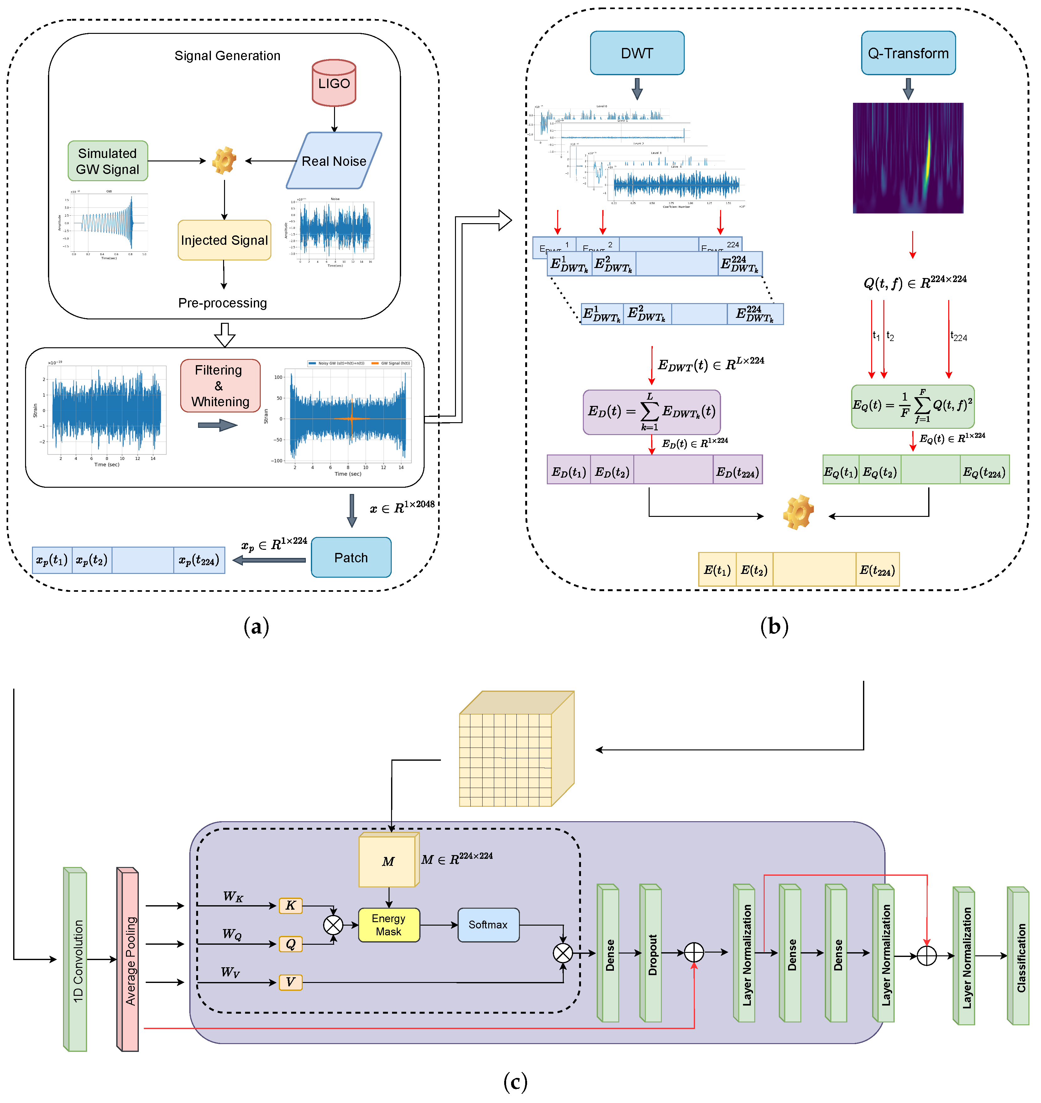
In this study, we propose a method to fuse physically interpretable energy representations of GW signals derived from Q-transform and DWT and integrate into a Transformer-based neural network via an energy-guided attention mechanism. In addition to leveraging energy information, the model also processes raw time-series data by dividing it into non-overlapping patches, which enables the Transformer to learn temporal features directly from the signal.
First, the raw gravitational-wave signal of length 2048 is subjected to preprocessing and subsequently transformed into a time–frequency representation using Q-transform. The Q-transform spectrogram, with a size of 224 × 224 , is processed to compute a one-dimensional energy vector, E q ( t ) , by averaging the squared magnitudes across all frequency bins for each time frame.
Moreover, the same signal is decomposed using DWT up to five levels to obtain wavelet coefficient arrays { c k } k = 1 5 . Each coefficient vector is squared, normalized, and resized to length 224 via interpolation to match the temporal scale of E q ( t ) . The Q-transform and DWT-based energy vectors are then fused into a single combined energy vector, E fuse ( t ) , by averaging all six vectors. This combined energy vector is used to compute a two-dimensional attention mask M by taking the outer product of E fuse ( t ) with itself. This mask is used to encode the pairwise temporal relevance of signal segments and modulates the attention weights in the Transformer.
On the other hand, the raw input signal is partitioned into 224 non-overlapping patches, each of length nine. These patches are passed through a 1D convolutional layer with ReLU activation, followed by average pooling, resulting in patch embeddings of dimension 128. These embeddings are given as input into the Transformer encoder including multi-head self-attention layers and feedforward networks. Unlike standard self-attention, the dot-product similarity matrix in EDAT-BBH is modulated by the energy mask M before applying the softmax operation. This ensures that the model focuses on signal regions that contain significant energy and contain meaningful information. Finally, the output corresponding to the first patch is passed through a dense layer with a sigmoid activation.
This methodology enables the EDAT-BBH model to exploit both global and local signal characteristics while embedding domain-specific priors directly into its attention mechanism, resulting in robust performance under noisy observational conditions.
Figure 1 shows the overall architecture of the proposed EDAT-BBH model. As shown in the figure, the pipeline consists of three main stages. Figure 1a shows the signal generation and pre-processing. Simulated BBH signals are injected into real LIGO noise and undergo whitening and patchification. Figure 1b illustrates energy mask construction using DWT and Q-transform. Independent energy representations are extracted from both wavelet and time–frequency domains and fused to construct an attention-guiding energy mask. This mask is then applied in a modified scaled dot-product attention mechanism in order to allow the model to focus on important temporal regions. Figure 1c shows the Transformer encoder with energy-modulated attention.

2.2. Q-Transform

Q-transform is a widely used technique in time–frequency analysis, demonstrating exceptional performance in signal processing. This method enables high-resolution representation of signals in both time and frequency domains, offering significant advantages in analyzing transient and localized events. Q-transform is a signal processing technique closely related to the short-time Fourier transform (STFT). It facilitates the conversion of a signal from the time domain to a time-–frequency representation. Despite the similarity between Q-transform and STFT, a key distinction lies in the geometric spacing of the center frequencies in Q-transform frequency bins. The Q-transform of a signal is mathematically expressed as follows [34]:
Q T ( k , n ) = j = n N k 2 n + N k 2 q ( j ) a k j n + N k 2 .
Here, q ( j ) represents a discrete-time signal, and k = 1 , 2 , , K corresponds to the frequency bins. In the above equation, a k ( n ) represents a basis function, commonly referred to as time–frequency atoms. The asterisk symbol ( ) denotes the complex conjugation operation, where a k ( n ) is the complex conjugate of a k ( n ) . The formulation of time–frequency atoms a k ( n ) is expressed as follows
a k ( n ) = 1 N k ω n N k e i 2 π n f k / f s ,
where f k stands for the center frequency corresponding to the k-th frequency bin, while f s denotes the sampling frequency. Finally, the term ω ( t ) represents a window function.
In practice, the constant Q parameter ensures that the transform adapts to the features of the signal. This property provides finer resolution where needed. For example, in high-frequency regions, the transform uses short-duration wavelets, capturing rapid changes in time. On the other hand, in low-frequency regions, the transform employs longer wavelets, capturing detailed spectral variations. For instance, in gravitational-wave analysis, Q-transform effectively characterizes transient features of gravitational waves near the event horizon in both time and frequency domains.
Figure 1. Overview of the proposed EDAT-BBH architecture. (a) Signal generation and pre-processing. The resulting signal is partitioned into 224 non-overlapping patches. (b) Energy mask construction. The preprocessed signal is independently passed through DWT and Q-transform operations. Energy representations are computed and fused to generate the energy mask M R 224 × 224 . (c) Energy-modulated attention mechanism. The input patches are embedded via 1D convolution and average pooling and then multi-head self-attention is modulated by the fused energy mask.
Electronics 14 04098 g001

2.3. Wavelet Coefficients

Wavelet transform is a representation and analysis of signals in both the time and frequency domains simultaneously. Unlike Fourier transforms, which decompose a signal into infinite-duration sinusoids, wavelet transform uses short and finite-length wavelets. Additionally, wavelet transforms analyze signals at multiple scales using localized waveforms. This multi-resolution property makes wavelet transforms particularly effective for analyzing non-stationary signals.
The wavelet transform represents a signal s ( t ) as a series of scaled and translated versions of a chosen mother wavelet function. Let ψ ( t ) be a wavelet function; then the continuous wavelet transform (CWT) of a signal s ( t ) is defined as
W ( a , b ) = s ( t ) ψ a , b ( t ) d t ,
where a is scale parameter using to control the dilation or compression of the wavelet and b is the translation parameter which determines the location of the wavelet in time. In (3), ( · ) denotes the complex conjugation operation. On the other hand, ψ a , b ( t ) represents the scaled and translated wavelet and given by
ψ a , b ( t ) = 1 a ψ t b a .
As seen from the equation above, the scale parameter a inversely relates to frequency. This parameter allows the wavelet transform to adapt its resolution dynamically. At low frequencies, the wavelet captures broad, smooth features of the signal, while at high frequencies, it detects sharp and localized details. On the other hand, the DWT samples the scale and translation parameters in discrete time and the DWT is expressed as
c m , n = s ( t ) ψ m , n ( t ) d t ,
where ψ m , n ( t ) = 2 m / 2 ψ ( ( 1 / 2 m ) ( t 2 m n ) ) , and m and n are integers representing the scale and translation indices, respectively. In addition, c m , n denotes the wavelet coefficients which represents the projection of the signal onto the wavelet basis functions at different scales and translations. They can be categorized into approximation and detail coefficients, which are represented as c A and c D , respectively. Approximation coefficients represent the low-frequency components of the signal. These coefficients capture the overall structure or trend of the signal. On the other hand, detail coefficients of the signal denote the high-frequency, small-scale components which capture localized variations or sharp transitions in the signal.

2.4. Transformer Architecture and Multi-Head Attention

The Transformer architecture, introduced in [35], has become a fundamental framework in deep learning due to its ability to model long-range dependencies without relying on recurrence. Therefore, the properties of Transformers make them widely successful in natural language processing [36,37], speech analysis [38], and, more recently, computer vision [39].
Transformers were initially designed for sequence-based tasks such as natural language processing, and they have been successfully adapted for other research areas. The key innovation of the Transformer is its self-attention mechanism, which provides the ability to capture relationships within sequential or spatial data. In [38], the authors demonstrated that self-attention could replace recurrent neural networks for efficient sequence-to-sequence modeling and [39] have shown that Transformers can outperform CNNs in image recognition tasks by applying self-attention over image patches. Therefore, the self-attention mechanism forms the backbone of Transformer architectures. It computes a weighted representation of input features by measuring the relationships between all elements of a sequence. Attention in Transformers is defined as
Attention ( Q , K , V ) = softmax Q K d k V ,
where Q, K, and V are query, key, and value matrices, respectively. On the other hand, d k is the scaling factor that prevents vanishing or exploding gradients when Q and K are high-dimensional matrices.
The self-attention mechanism can be extended to the multi-head attention mechanism. In this mechanism, each head independently applies the scaled dot product attention and projects the outputs back into the feature space. This process can be explained as follows:
MultiHead ( Q , K , V ) = Concat ( head 1 , head 2 , , head h ) W O ,
where each attention head is given by
head i = Attention ( Q W i Q , K W i K , V W i V ) .
Here, W i Q R n × d k , W i K R n × d k , and W i V R n × d v are learnable projection matrices for the i-th head, and W O R h · n × d k is the output projection matrix. On the other hand, n represents the dimension of input and d k is the dimensionality of the query and key vectors. By attending to multiple aspects of the input sequence in parallel, multi-head attention enables the model to capture complex dependencies [35].

2.5. Bayesian-Optimized Energy-Modulated Transformer

In this study, we utilized Bayesian optimization to find the optimum architecture and hyperparameters of an EDAT-BBH model for a binary classification task. Bayesian optimization leverages a probabilistic model to predict the performance of a machine learning algorithm given specific hyperparameters. This approach has the advantage of optimizing high-dimensional objective functions in deep learning models. Additionally, it also allows us to systematically explore the hyperparameter space and find an architecture that achieves an optimal trade-off between model complexity and generalization.
The idea behind Bayesian optimization is to find the optimum value of a black-box objective function, f ( x ) , where x represents the hyperparameters. Hence, the global optimization problem can be expressed as follows.
x = arg max x X f ( x ) ,
where x = [ x 1 , x 2 , , x t ] and x denote the optimum values. Let D = { x , f ( x ) } represent the previous observation and { x t + 1 , f ( x t + 1 ) } denote the new observation taken from the same sample space, where x t + 1 is the next sample point. According to the properties of Gaussian process, f ( x ) and f ( x t + 1 ) are jointly Gaussian. Then, the predictive distribution can be expressed as [40]
P ( f t + 1 D 1 : t , x t + 1 ) = N μ t ( x t + 1 ) , σ t 2 ( x t + 1 ) .
Here μ t ( x t + 1 ) and σ t 2 ( x t + 1 ) are predictive mean and variance, respectively. Let k ( x n , x n ) represent the covariance function and K denote the covariance matrix as follows:
K = k ( x 1 , x 1 ) k ( x 1 , x t ) k ( x t , x 1 ) k ( x t , x t ) .
Then, the predictive mean and variance are written by
μ t ( x t + 1 ) = k K 1 f 1 : t , σ t 2 ( x t + 1 ) = k ( x t + 1 , x t + 1 ) k K 1 k .
where k = k ( x t + 1 , x 1 ) , k ( x t + 1 , x 2 ) , , k ( x t + 1 , x t ) .
Bayesian optimizations utilize the acquisition functions, α ( · ) , to find the best x t + 1 . For this purpose, several acquisition functions exist. However, in this study, we employ the Upper Confidence Bound (UCB) acquisition function which is given as follows:
α UCB ( x ) = μ ( x ) + κ σ ( x ) ,
where σ ( x ) is the standard deviation. After acquisition function is calculated, then the next point can be found by the using following optimization problem:
x t + 1 = arg max x X α UCB ( x ) .
In this study, Bayesian optimization was applied to determine the number of attention heads, the size of the feedforward layers, and the learning rate, resulting in a highly effective model configuration.

2.6. Proposed Method

In this study, we propose an Energy-Modulated Dual-Attention Transformer which is a novel Transformer-based architecture that utilizes physically interpretable energy representations to enhance the detection of GW signals. Unlike the conventional Transformer models, the EDAT-BBH method proposed in this study introduces domain-specific information extracted from time–frequency and multi-resolution analyses in order to modulate the attention mechanism.
In this study, real noise signals are obtained from the LIGO detector and all signals are sampled at a rate of 2048 Hz. In our simulations, we utilize 1 s long segments. Therefore, each signal used in this study has 2048 samples. Let s denote a single signal sample, and s ^ is a filtered and whitened signal obtained for reducing non-physical artifacts. Then, the pre-processed signal can be expressed as a sequence of discrete time-domain values as s ^ = { s ^ 1 , s ^ 2 , , s ^ 2048 } . Alternatively, this signal can be represented in a more compact form as { s ^ n } n = 1 2048 , where n represents the total number of time-domain samples in the signal.
First of all, in order to compute the time–frequency representation of the signal s ^ , Q-transform is employed by using Equation (1). In this way, 2D images are obtained with a resolution of 224 × 224 , and these images are represented as Q T ( t , f ) R 224 × 224 . After that, Q-transform images of signals are used to extract one-dimensional energy vector by averaging the squared magnitude of each time–frequency pixel across all frequency bins as follows:
E q ( t ) = 1 F f = 1 F Q T ( t , f ) 2 ,
where F = 224 is the number of frequency bins and E q ( t ) R 224 represents the energy vector. Then, the resulting vector E q ( t ) is normalized to the range [ 0 , 1 ] .
Secondly, in order to obtain high-energy DWT features, the signal s ^ is first decomposed into four-level DWT coefficients. A four-level decomposition produces four sets of detail coefficients ( D 1 D 4 ) and one set of approximation coefficients (A), which form a total of L = 5 sub-bands represented as { c k } k = 1 5 . For each level k, the energy vector is computed by squaring the coefficients as E c k ( t ) = c k ( t ) 2 . Then, E c k is normalized as
E c k N ( t ) = E c k ( t ) min ( E c k ( t ) ) max ( E c k ( t ) ) min ( E c k ( t ) ) .
After normalization, E c k N ( t ) is resized to length 224 using interpolation to obtain the DWT energy vector, E ˜ c k ( t ) . This ensures alignment between all energy vectors in the time dimension. Then, the energy vectors obtained by Q-transform given in (15) and the DWT given in (16) are combined to form dual-energy vector as follows:
E fuse ( t ) = 1 L + 1 α E q ( t ) + ( 1 α ) k = 1 L E ˜ c k ( t ) ,
where L = 5 and α represent the weighting factor between the Q-transform and DWT energy vectors. To construct the attention mask, the outer product of the combined vector is calculated as
M ( i , j ) = E fuse ( i ) E fuse ( j ) .
In this way, the mask matrix M R 224 × 224 is obtained for masking the embedding matrix in the attention mechanism, where M ( i , j ) denotes the element of M at the i-th row and j-th column. As shown in Figure 1, after constructing the energy mask matrix M , the attention mechanism is modified by element-wise multiplication of attention scores with the mask M . This modification allows the model to emphasize the important regions of the signal. The masked attention outputs are then passed through residual connections, layer normalization, and feedforward networks within the Transformer encoder blocks.

2.7. Signal Patch Embedding and Attention Modulation

The filtered and whitened signal s ^ R 2048 × 1 is partitioned into 224 non-overlapping patches of length 10. Each patch is processed by a one-dimensional convolutional layer with ReLU activation. Then, average pooling is applied to the output of the convolution layer to yield a patch embedding matrix Z R 224 × d where d = 128 . These patch embeddings are passed to a Transformer encoder. Unlike standard Transformers, proposed model in this study incorporates an energy-based modulation mechanism. Specifically, the scaled dot-product attention is element-wise modulated using an attention mask M derived from physical signal energy distributions. The resulting modified attention formulation is defined as follows
Attention ( Q , K , V ) = Softmax Q K d k M V
where ⊙ denotes the Hadamard (element-wise) product.
We call this algorithm EDAT-BBH (Energy-Modulated Dual-Attention Transformer for Binary Black Hole classification). A generic pseudocode that has been proposed for the classification of a binary black hole signal can be found in Algorithm 1.
Algorithm 1 EDAT-BBH: Energy-Modulated Dual-Attention Transformer for Binary Black Hole classification
  1:
Filter and whiten the BBH signal s and obtain s ^
Step 1: Energy Extraction from Q-transform
  2:
Q T ( k , n ) = j = n N k 2 n + N k 2 s ^ ( j ) a k j n + N k 2 .
  3:
E q ( t ) = 1 F f = 1 F Q T ( k , n ) 2
  4:
E ˜ q ( t ) = E q ( t ) min ( E q ) max ( E q ) min ( E q )
Step 2: Energy Extraction from DWT Coefficients
  5:
for each level k = 1 to L do
  6:
     E c k ( t ) = c k ( t ) 2
  7:
     E c k N ( t ) = E c k ( t ) min ( E c k ( t ) ) max ( E c k ( t ) ) min ( E c k ( t ) )
  8:
     E ˜ c k ( t ) = I n t e r p o l a t i o n ( E c k N ( t ) )
  9:
end for
Step 3: Energy Mask Construction
 10:
E fuse ( t ) = 1 L + 1 α E ˜ q ( t ) + ( 1 α ) k = 1 L E ˜ c k ( t )
 11:
M ( i , j ) = ( E ˜ fuse ( i ) ) ( E ˜ fuse ( j ) )
Step 4: Signal Patchification and Embedding
 12:
Split s ^ R 2048 × 1 into 224 patches of size 9
 13:
Apply Conv1D + AveragePooling1D for embedding
Step 5: Transformer Encoder with Energy Modulation
 14:
for each attention layer do
 15:
     Attention ( Q , K , V ) = Softmax Q K d k M V
 16:
    Apply residual connection + LayerNorm
 17:
    Apply fully connected network + residual connection + LayerNorm
 18:
end for
Step 6: Classification Head
 19:
y ^ = σ ( W · CLS + b )
Step 7: Loss and Optimization
 20:
Compute binary crossentropy loss
 21:
Update model parameters using Adam optimizer

2.8. Classification Output

Finally, the processed feature representations are passed through a classification layer to produce the final classification output and distinguish gravitational-wave signals from noise. Moreover, in order to optimize the proposed performance of the model, Bayesian optimization is employed to find the optimum hyperparameters, such as the number of transformer heads, learning rates, and dropout rates, ensuring efficient and robust detection of BBH signals from LIGO data. Following the Transformer blocks, the embedding corresponding to the first patch position (CLS token) is extracted and passed through a dense output layer with sigmoid activation to produce a binary prediction as
y ^ = σ ( W z 0 + b ) ,
where z 0 is the embedding at index 0.

3. Results

In this study, all simulations are employed using the Google Colaboratory (Google Colab) platform, which provides cloud-based computational resources. On this platform, an NVIDIA A100 Tensor Core GPU (NVIDIA, Santa Clara, CA, USA) was utilized to accelerate the computations with a memory of 80 GB. It enables efficient processing of large-scale datasets and deep learning models. Additionally, the platform provides access to RAM with a memory of 83.5 GB.

Dataset

In this study, we aim to detect gravitational signals collected from a noisy environment. Therefore, the problem we are interested in is a kind of classification problem where the signals are classified into signal and noise. As the first step of collecting data, we use real data obtained from the LIGO recordings instead of using synthetic Gaussian noise. For this purpose, noise signals are extracted from observing run O1 in the LIGO detector. This dataset is publicly available in the Gravitational Wave Open Science Center (GWOSC) [41,42]. On the other hand, for positive samples, GW signals from black hole mergers were simulated using the PyCBC library by employing the SEOBNRv4_opt waveform model, which accurately represents the time-domain evolution of the signals during the merger. The masses of the two black holes were randomly chosen from the uniform distribution within the range of 10 to 80 solar masses, which provides a broad parameter space. This mass range was designed to align with the observed data and increase the diversity of the simulated signals. On the other hand, the dimensionless spin components along the z-axis were also randomly selected within the range of 0 to 0.998. For filtering, a lower frequency cutoff of 20 Hz was applied to filter out components below this threshold. After that, each signal was generated to be 1 s in duration and was processed at a sampling rate of 2048 Hz. Therefore, each signal in our generated dataset has 2048 samples.
To create a realistic dataset, these signals were injected into background noise obtained from LIGO observations. All simulated BBH signals were injected into real LIGO detector noise in order to preserve the non-stationary and non-Gaussian features of the background, including instrumental and environmental noise, thereby ensuring that the performance evaluation reflects realistic observational conditions. Let n ( t ) be a detector noise and h ( t ) denotes the GW signals. Then, the GW strain can be represented as
s ( t ) = h ( t ) + n ( t )
Each h ( t ) signal is obtained by scaling the template signal to a specific signal-to-noise ratio (SNR) and injected into the LIGO background noise. The optimal SNR value can be written as follows [43]:
ρ 2 = 4 0 | H ( f ) | 2 S n ( f ) d f ,
where S n ( f ) and H ( f ) represent the estimated power spectral density of noise and the Fourier transform of h ( t ) , respectively. In order to obtain the injected signals, the SNR values are selected randomly from the uniformly distributed range of 8 to 30. Then, the scaled signal is injected into the background noise in order to simulate realistic gravitational waves. This method enhanced the diversity and physical realism of the GW signals while enabling the construction of a balanced and realistic dataset for training machine learning models. After signals injected into background noise, final signals are whitened by employing the estimated power spectral density of signal. Then, whitened signal is filtered using bandpass filter between 30 and 512 Hz. Specifically, the raw detector strain is dominated by strong low-frequency noise. In the time domain, this appears as large, slow oscillations that obscure the gravitational-wave signal. To mitigate this, we first apply whitening using a local estimate of the power spectral density. The whitening process flattens the noise spectrum and equalizes the contribution of different frequency bins. This suppresses regions with excess noise and allows the subsequent time–frequency representation to reflect the intrinsic signal content more faithfully. Without whitening and filtering, any time–frequency or wavelet transform applied to the raw strain would be dominated by the strong noise background, causing the true GW signal content to be heavily masked. Therefore, whitening and preprocessing are essential to obtain energy vectors that faithfully represent the physical properties of the underlying signals. In this way, 20,000 one-second signals are obtained and classification was performed using 10,000 signal samples and 10,000 noise samples.
Figure 2a,b show the real noise segment obtained from LIGO and simulated gravitational GW signal, respectively. As seen from Figure 2a, real noise consists of random fluctuations caused by environmental and instrumental reasons. On the other hand, the GW waveform given in Figure 2b represents the expected signal from a BBH event. This signal is a short-duration, chirp-like waveform, characterized by an increasing frequency and amplitude over time, which is a signature feature of compact binary coalescence events. However, the short duration of the GW signal poses a challenge for its detection within long stretches of noisy data. On the other hand, Figure 2c,d demonstrate the noise after filtering and overlay the filtered and whitened noise with the simulated GW signal, respectively.
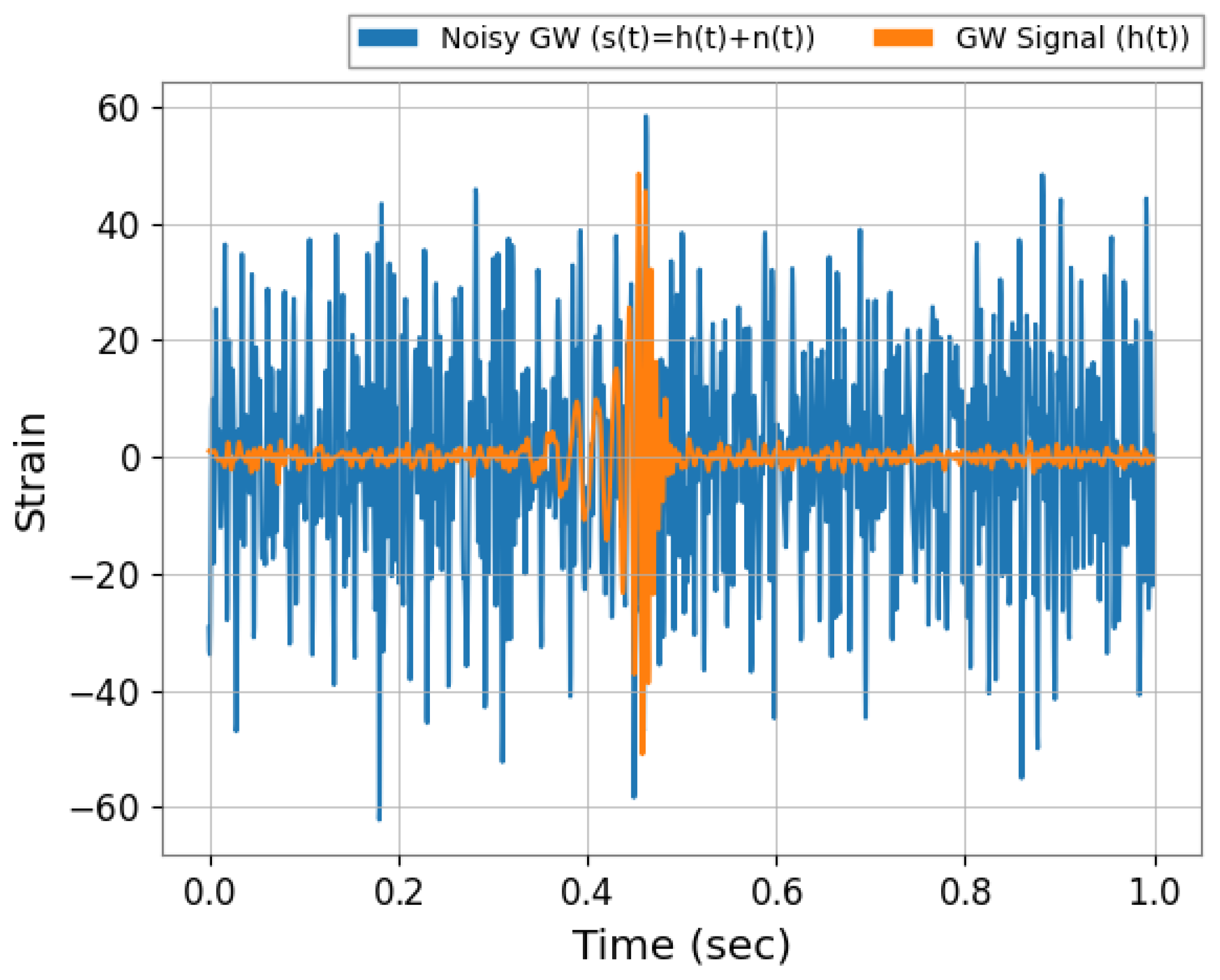
In this study, the data is divided into 1 s segments. During the generation of simulated data, the GW signal is randomly placed around the center of each 1 s noise segment within ± 0.3 s of the center. This random placement introduces variability in the training data to improve their generalization ability across different noise conditions and signal properties. Figure 3 shows an example of the 1 s long filtered and whitened noise and GW data used to train the deep learning model.
The dataset used in this study consists of time series signals. Let D = { ( s n , y n ) s n R 1 × 2048 , y n { 0 , 1 } } denote the dataset where each s n is an individual time series data point of dimension 1 × 2048 with a corresponding binary label. Here, n = 1 , , N , and N represent the total number of samples which have a 1 × 2048 sequence. Since the dataset utilized in this study includes a total of 20,000 samples, N = 20 , 000 . These samples are divided between two distinct categories. The first subset consists of 10,000 samples containing generated BBH merger signals that have been injected with different SNR values into real noise samples collected from LIGO detectors. In this way, these injections are generated to mimic astrophysical sources with parameters representative of realistic BBH systems. The second subset includes 10,000 samples of real detector noise obtained from the LIGO. This real noise ensures a realistic evaluation of signal detection methodologies.
The effect of varying SNR values on the time–frequency representation of gravitational-wave signals can be seen in Figure 4. At low SNR, the signal is visually indistinguishable from background noise, as given in Figure 4a,b. However, as shown in Figure 4c,d, a chirp-like GW signal emerges and becomes clearly visible with increasing SNR values.
In our simulations, the dataset is divided into batches and the batch size is selected as 32. To train and evaluate the performance of the model, the dataset was split into training, validation, and test sets, with 70% (14,000 samples) allocated for training, 10% (2000 samples) for validation, and the remaining 20% (4000 samples) for testing, and the epoch number is chosen as 100. Additionally, the Bayesian optimization method is utilized in order to find the optimum model architecture. The training parameters determined by Bayesian optimization are given in Table 1.
Bayesian hyperparameter optimization was employed to tune both the Transformer and CNN components of the proposed architecture. In the search space, the number of attention heads was varied between two and eight, the dimensionality of each attention head was selected among 32, 64, and 128, and the size of the feedforward network was searched within the range of 64 to 256 with increments of 32. The number of Transformer encoder blocks was allowed to vary between one and four. For the convolutional layers, the number of stacked layers was set between one and four, with the number of filters in each layer selected from 16 to 128 in increments of 16. The kernel size was fixed at 3 × 3 across all convolutional layers. Additionally, dropout rates were sampled in the range 0.1 to 0.5 with a step size of 0.1, while the learning rate was searched on a logarithmic scale between 1 × 10 4 and 1 × 10 2 . The optimization process was carried out with 60 trials and each candidate configuration was trained for 100 epochs using early stopping criteria.
As a result of Bayesian optimization, the model was configured with four attention heads, two transformer encoder layers, a dropout rate of 0.2, and a learning rate of 10 4 . Moreover, in the model, each patch is processed through convolutional layers with a kernel size of three and 128 filters, followed by an average pooling operation.
To evaluate the classification performance, the EDAT-BBH model was benchmarked against several state-of-the-art methods using several performance metrics such as accuracy, precision, F1-score, recall, ROC AUC, and PR AUC. Table 2 presents a comperative analysis between the proposed model and the prior models given in [5,6]. The results indicate that the proposed model outperforms all competing models in terms of performance metrics. Proposed method achieves the best overall classification accuracy of 0.9953. Additionally, it achieves the highest recall and F1-score. Moreover, in terms of metrics for area under the curve, the proposed model achieves the best scores in both ROC AUC and PR AUC.
Table 3 presents the performance of the EDAT-BBH compared to CoT-temporal and CoT-spectral in terms of F1-score and AUC as evaluation metrics as given in [8]. CoT-temporal and CoT-spectral are also Transformer-based models proposed for classificaiton of GW signals. EDAT-BBH significantly outperforms both CoT-temporal and CoT-spectral models in both metrics. CoT-temporal and CoT-spectral models achieve F1-scores of 0.9140 and 0.9160, with AUC values of 0.9350 and 0.9380, respectively. On the other hand, EDAT-BBH achieves an F1-score of 0.9953 and AUC of 0.9999.
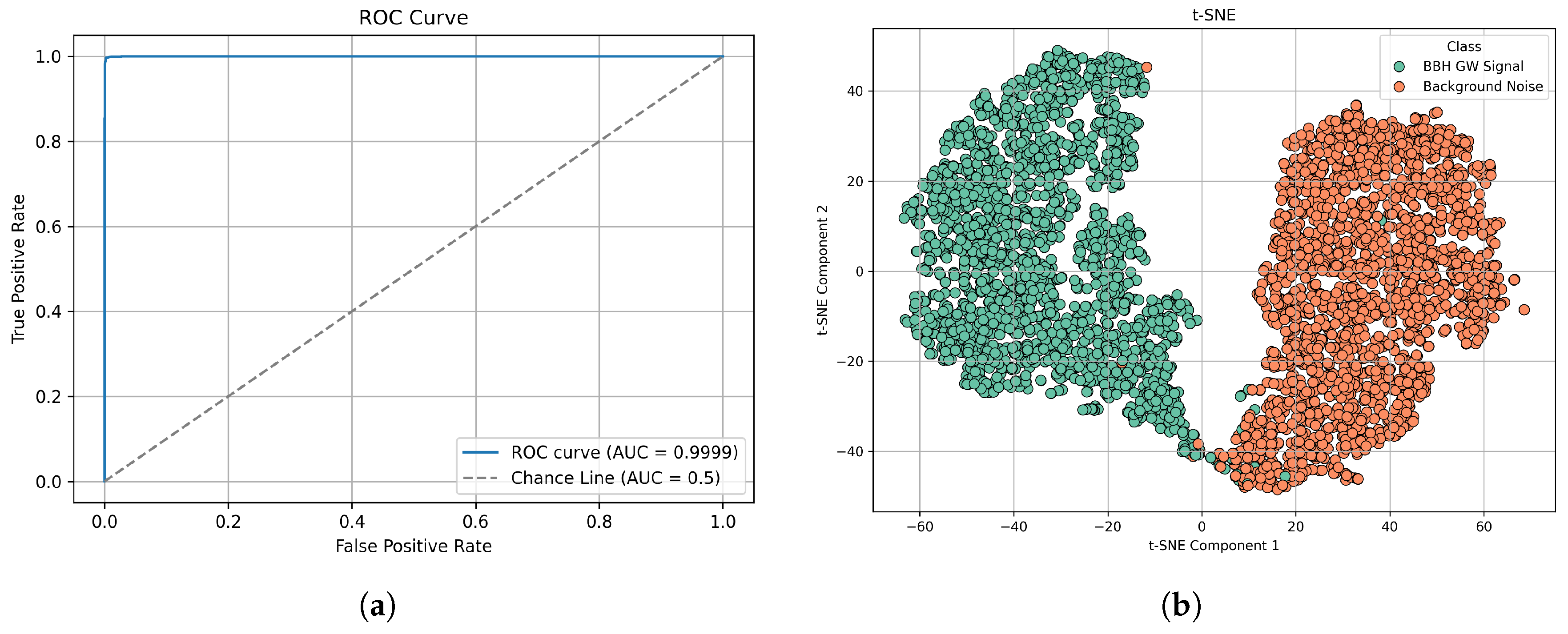
Figure 5 presents the ROC curve and t-SNE projection to illustrate the classification performance of the model. As shown in the figure, the proposed EDAT-BBH model demonstrates effective binary classification performance. The ROC curve given in Figure 5a shows an area under the curve (AUC) of 0.9998. Additionally, the t-SNE projection demonstrated in Figure 5b visualizes the learned high-dimensional representations. Separation between background noise and BBH signal using the EDAT-BBH model can be seen in Figure 5b.
Table 4 demonstrates the systematic comparison of Q-transform and DWT fusion across different weighting factors ( α ) to quantify both central performance (accuracy, precision, recall, F1, ROC–AUC) and robustness (standard deviation and %95 confidence intervals) and to contrast fusion against single-modality baselines (only Q-transform and only DWT). By presenting these variants side by side, the table is intended to reveal whether balanced fusion improves performance and stability and to inform a sensible default choice of α for practical use.

4. Discussion

The results, as given in Table 2 and Table 3 and Figure 5 and Figure 6, demonstrate the advantages of energy-guided attention over traditional and recent Transformer-based approaches.
As shown in Table 2, the EDAT-BBH model outperforms all comparative baselines, including well-known CNN-based models such as EfficientNet and Xception. It achieves the highest accuracy, F1-score, and AUC metrics. In Table 3, the proposed model is compared against CoT-temporal and CoT-spectral Transformers. The performance of CoT-based models remains significantly below that of EDAT-BBH. This shows that using physical energy distributions to guide attention helps the model find important time regions more effectively than using fixed rules based only on time or frequency.
Table 4 indicates that fusing Q-transform and DWT features yields better and more stable performance than either modality alone. As the fusion weight moves toward α = 0.5 , accuracy and F1-score reach their highest levels. Moreover, precision is also peaking at this weighting value. The low standard deviations and narrow CI reflects consistent behavior of models across folds. According to the results, DWT only is closer to fusion than using only Q-transform, yet it still falls short of the stability and performance achieved at α = 0.5 .
The performance metrics and visualizations provided in Figure 5 show the effectiveness of the EDAT-BBH model. Moreover, the t-SNE projection of the learned CLS token embeddings provides an interpretable representation of how well the model separates different classes in space. This separability can be attributed to the energy-aware attention mechanism, which adaptively emphasizes important regions during learning. These results confirm not only the predictive performance of the model but also its internal representation for gravitational-wave detection.
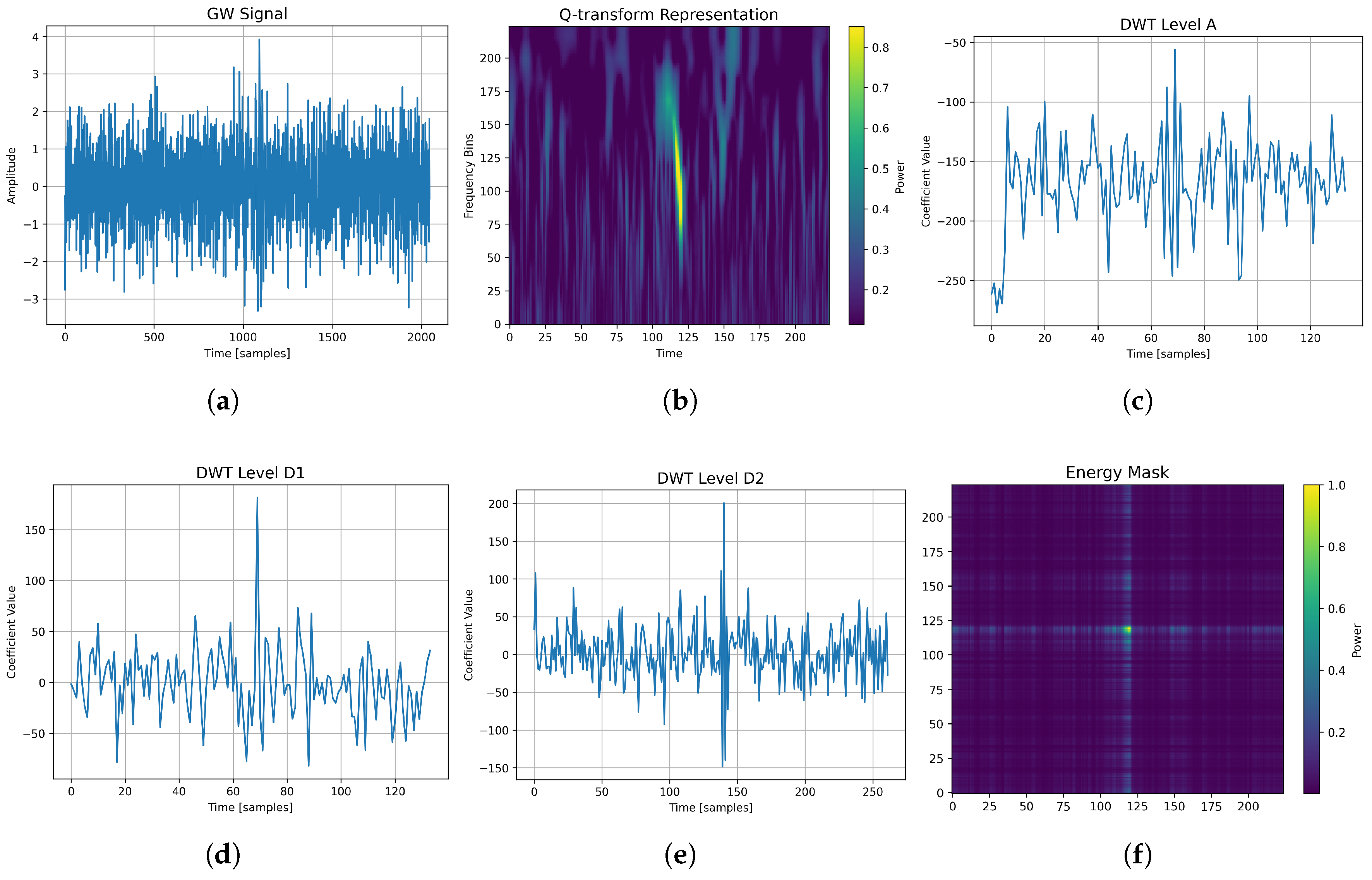
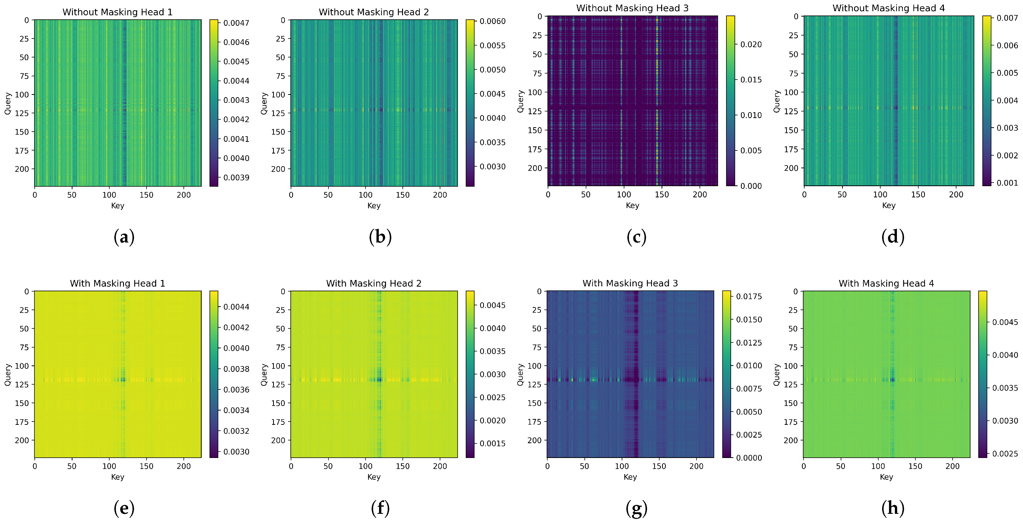
In order to show the effect of applying modulation masks, we present Figure 6 and Figure 7 using a sample of input signals. Figure 6a illustrates a sample of the input signal, Figure 6b shows the Q-transform representation of the input signal, and Figure 6c–e illustrate the DWT decompositions of the signal. Finally, in Figure 6f the fused energy mask is given. The energy mask preserves the temporal locality and frequency sensitivity of the signal, which enables the Transformer to focus on important regions for candidate events. Moreover, Figure 7 provides a comparison of attention maps with and without energy masking. Figure 7a–d depict the attention map from each of the four heads in the absence of masking. As seen in these figures, there is a lack of clear localization. In contrast, Figure 7e–h show attention maps after energy modulation. Here, attention is concentrated on specific regions associated with high energy. These figures show how the energy mask effectively guides the model toward the most relevant parts of the signal. Additionally, masking also suppresses the irrelevant attention regions.
Table 5 presents a paired comparison between Transformer models with and without energy masking across attention–SNR correlation, IoU, and entropy. Additionally, paired Wilcoxon signed-rank p-values are given to assess statistical significance. In order to compute the attention–SNR metrics, we first min–max normalize the attention map A R 224 × 224 and the corresponding Q-transform Q T R 224 × 224 to [0, 1]. The attention–SNR correlation is then computed as the Spearman rank correlation between vec ( A ) and vec ( Q T ) . To measure spatial overlap, we binarize A by keeping its top 5 % values and Q T by keeping its top 5 % energy, and we compute the IoU. Finally, attention entropy is computed as H ( A ) = j p j log p j with p j = A j / k A k . As seen from the table, energy masking yields consistent and statistically reliable improvements. The attention–SNR correlation, which is negative without masking, becomes positive with energy masking. This result indicates a realignment of attention toward high-SNR regions. IoU also increases with the use of an energy mask, demonstrating improved spatial overlap with target regions. Although the increase in IoU seems small, it corresponds to a relative improvement of approximately 37% compared to the no-masking condition. On the other hand, a reduction in entropy indicates sharper and more concentrated attention distributions. In addition, as shown in the table, all paired differences are significant according to the p-values.
The computational performance results presented in Table 6 highlight substantial differences in computational efficiency, model complexity, and inference performance among the evaluated architectures. ResNet101, Xception, and EfficientNetB0 exhibit significantly higher parameter counts (42.7 M, 20.9 M, and 4.1 M, respectively) and floating-point operation requirements (15.2 G, 9.1 G, and 0.8 G, respectively) compared to the proposed EDAT-based models (0.216 M parameters, 0.154 G FLOPs). Moreover, in terms of latency (ms/sample), the EDAT models achieved low inference times of approximately 41–42 ms for a batch size of 1 and 3.8–5.3 ms for a batch size of 32. Therefore, the EDAT model outperforms the baseline CNNs. This improvement translated into substantially higher throughput. While the standard backbones reached between 2.2 and 7.6 samples/s at batch size 1, the EDAT models attained 23.5–23.8 samples/s. At batch size 32, the throughput advantage became even more pronounced, with EDAT achieving 417–513 samples/s compared to 40–90 samples/s for the CNN models. The inclusion of the proposed energy-based attention mask in EDAT incurred only a marginal increase in latency (≈0.6 ms at bs = 1). According to the Table 6, the EDAT architecture not only delivers competitive predictive performance but also it is highly suitable for real-time or resource-constrained gravitational-wave detection scenarios where low latency and high throughput are critical.

5. Conclusions

In this study, we introduce EDAT-BBH, a novel Transformer-based architecture that leverages energy-driven attention modulation for binary black hole gravitational-wave signal classification. By integrating Q-transform and DWT-based energy representations into a unified attention mask, the model selectively focuses on high-information regions of the input signal while suppressing noise-dominated segments.
Simulation results demonstrate the superiority of EDAT-BBH over conventional CNN-based and Transformer-based baselines across all performance metrics. Beyond its strong classification performance, the model enhances interpretability by aligning attention distributions with physically meaningful energy patterns. The illustrated figures of the attention maps confirm the impact of energy masking in concentrating the focus of the model.
One of the primary advantages of energy-aware attention is its alignment with physically meaningful signal attributes. Unlike conventional attention mechanisms, the proposed approach incorporates energy as an inductive prior which results in more interpretable attention maps that correspond with known GW signal characteristics.
The success of EDAT-BBH highlights the potential of physics-informed attention modulation in deep learning architectures, especially for domains like gravitational-wave astrophysics where noise exhibits a non-stationary structure [44,45]. This approach can be further applied to areas such as multi-detector signal fusion.

Funding

This research received no external funding.

Data Availability Statement

Publicly available at the Gravitational Wave Open Science Center (GWOSC) [41,42].

Conflicts of Interest

The author declares no conflict of interest.

Abbreviations

The following abbreviations are used in this manuscript:
GWGravitational Wave
LIGOLaser Interferometer Gravitational-Wave Observatory
BBHBinary Black Hole
GWOSCGravitational Wave Open Science Center

References

  1. Einstein, A. Approximative Integration of the Field Equations of Gravitation. Sitzungsberichte KöNiglich PreußIschen Akad. Wiss. Berl. (Math. Phys.) 1916, 1916, 688–696. [Google Scholar]
  2. Observation of Gravitational Waves from a Binary Black Hole Merger. 2016. Available online: https://journals.aps.org/prl/covers/116/6 (accessed on 23 April 2022).
  3. Accadia, T.; Acernese, F.; Antonucci, F.; Astone, P.; Ballardin, G.; Barone, F.; Barsuglia, M.; Bauer, T.S.; Beker, M.; Belletoile, A.; et al. Noise from Scattered Light in Virgo’s Second Science Run Data. Class. Quantum Gravity 2010, 27, 194011. [Google Scholar] [CrossRef]
  4. Abbott, B.P.; Abbott, R.; Abbott, T.; Abernathy, M.; Acernese, F.; Ackley, K.; Adamo, M.; Adams, C.; Adams, T.; Addesso, P.; et al. Characterization of Transient Noise in Advanced LIGO Relevant to Gravitational Wave Signal GW150914. Class. Quantum Gravity 2016, 33, 134001. [Google Scholar] [CrossRef]
  5. Lopac, N.; Hrzic, F.; Vuksanovic, I.P.; Lerga, J. Detection of Non-Stationary GW Signals in High Noise From Cohen’s Class of Time–Frequency Representations Using Deep Learning. IEEE Access 2022, 10, 2408–2428. [Google Scholar] [CrossRef]
  6. George, D.; Huerta, E.A. Deep Learning for Real-Time Gravitational Wave Detection and Parameter Estimation: Results with Advanced LIGO Data. Phys. Lett. B 2018, 778, 64–70. [Google Scholar] [CrossRef]
  7. Benedetto, V.; Gissi, F.; Ciaparrone, G.; Troiano, L. AI in Gravitational Wave Analysis, an Overview. Appl. Sci. 2023, 13, 9886. [Google Scholar] [CrossRef]
  8. Jiang, L.; Luo, Y. Convolutional Transformer for Fast and Accurate Gravitational Wave Detection. In Proceedings of the 2022 26th International Conference on Pattern Recognition (ICPR), Montreal, QC, Canada, 21–25 August 2022; pp. 46–53. [Google Scholar]
  9. Gebhard, T.D.; Kilbertus, N.; Harry, I.; Schölkopf, B. Convolutional Neural Networks: A Magic Bullet for Gravitational-Wave Detection? Phys. Rev. D 2019, 100, 063015. [Google Scholar] [CrossRef]
  10. Gabbard, H.; Williams, M.; Hayes, F.; Messenger, C. Matching Matched Filtering with Deep Networks for Gravitational-Wave Astronomy. Phys. Rev. Lett. 2018, 120, 141103. [Google Scholar] [CrossRef]
  11. Kim, K.; Li, T.G.F.; Lo, R.K.L.; Sachdev, S.; Yuen, R.S.H. Ranking Candidate Signals with Machine Learning in Low-Latency Search for Gravitational-Waves from Compact Binary Mergers. Phys. Rev. D 2020, 101, 083006. [Google Scholar] [CrossRef]
  12. Zevin, M.; Coughlin, S.; Bahaadini, S.; Besler, E.; Rohani, N.; Allen, S.; Cabero, M.; Crowston, K.; Katsaggelos, A.K.; Larson, S.L.; et al. Gravity Spy: Integrating Advanced LIGO Detector Characterization, Machine Learning, and Citizen Science. Class. Quantum Gravity 2017, 34, 064003. [Google Scholar] [CrossRef]
  13. Powell, J.; Torres-Forné, A.; Lynch, R.; Trifirò, D.; Cuoco, E.; Cavaglià, M.; Heng, I.S.; Font, J.A. Classification Methods for Noise Transients in Advanced Gravitational-Wave Detectors II: Performance Tests on Advanced LIGO Data. Class. Quantum Gravity 2017, 34, 034002. [Google Scholar] [CrossRef]
  14. George, D.; Shen, H.; Huerta, E. Classification and Unsupervised Clustering of LIGO Data with Deep Transfer Learning. Phys. Rev. D 2018, 97, 101501. [Google Scholar] [CrossRef]
  15. Cuoco, E.; Razzano, M.; Utina, A. Wavelet-Based Classification of Transient Signals for Gravitational Wave Detectors. In Proceedings of the 2018 26th European Signal Processing Conference (EUSIPCO), Rome, Italy, 3–7 September 2018; pp. 2648–2652. [Google Scholar]
  16. Bişkin, O.T.; Kirbaş, I.; Çelik, A. A Fast and Time-Efficient Glitch Classification Method: A Deep Learning-Based Visual Feature Extractor for Machine Learning Algorithms. Astron. Comput. 2023, 42, 100683. [Google Scholar] [CrossRef]
  17. Shen, H.; George, D.; Huerta, E.A.; Zhao, Z. Denoising Gravitational Waves with Enhanced Deep Recurrent Denoising Auto-Encoders. In Proceedings of the ICASSP 2019—2019 IEEE International Conference on Acoustics, Speech and Signal Processing (ICASSP), Brighton, UK, 12–17 May 2019; pp. 3237–3241. [Google Scholar]
  18. Torres-Forné, A.; Marquina, A.; Font, J.A.; Ibáñez, J.M. Denoising of Gravitational Wave Signals via Dictionary Learning Algorithms. Phys. Rev. D 2016, 94, 124040. [Google Scholar] [CrossRef]
  19. Wei, W.; Huerta, E.A. Gravitational Wave Denoising of Binary Black Hole Mergers with Deep Learning. Phys. Lett. B 2020, 800, 135081. [Google Scholar] [CrossRef]
  20. Vajente, G.; Huang, Y.; Isi, M.; Driggers, J.C.; Kissel, J.S.; Szczepańczyk, M.J.; Vitale, S. Machine-Learning Nonstationary Noise out of Gravitational-Wave Detectors. Phys. Rev. D 2020, 101, 042003. [Google Scholar] [CrossRef]
  21. Yan, R.Q.; Liu, W.; Yin, Z.Y.; Ma, R.; Chen, S.Y.; Hu, D.; Wu, D.; Yu, X.C. Gravitational Wave Detection Based on Squeeze-and-Excitation Shrinkage Networks and Multiple Detector Coherent SNR. Res. Astron. Astrophys. 2022, 22, 115008. [Google Scholar] [CrossRef]
  22. Chaturvedi, P.; Khan, A.; Tian, M.; Huerta, E.; Zheng, H. Inference-Optimized AI and High Performance Computing for Gravitational Wave Detection at Scale. Front. Artif. Intell. 2022, 5, 828672. [Google Scholar] [CrossRef]
  23. Goyal, S.; Kapadia, S.J.; Ajith, P. Rapid Identification of Strongly Lensed Gravitational-Wave Events with Machine Learning. Phys. Rev. D 2021, 104, 124057. [Google Scholar] [CrossRef]
  24. Moreno, E.A.; Borzyszkowski, B.; Pierini, M.; Vlimant, J.R.; Spiropulu, M. Source-Agnostic Gravitational-Wave Detection with Recurrent Autoencoders. Mach. Learn. Sci. Technol. 2022, 3, 025001. [Google Scholar] [CrossRef]
  25. Krastev, P.G. Real-Time Detection of Gravitational Waves from Binary Neutron Stars Using Artificial Neural Networks. Phys. Lett. B 2020, 803, 135330. [Google Scholar] [CrossRef]
  26. Schäfer, M.B.; Ohme, F.; Nitz, A.H. Detection of Gravitational-Wave Signals from Binary Neutron Star Mergers Using Machine Learning. Phys. Rev. D 2020, 102, 063015. [Google Scholar] [CrossRef]
  27. Miller, A.L.; Astone, P.; D’Antonio, S.; Frasca, S.; Intini, G.; La Rosa, I.; Leaci, P.; Mastrogiovanni, S.; Muciaccia, F.; Mitidis, A.; et al. How Effective Is Machine Learning to Detect Long Transient Gravitational Waves from Neutron Stars in a Real Search? Phys. Rev. D 2019, 100, 062005. [Google Scholar] [CrossRef]
  28. Astone, P.; Cerda-Duran, P.; Di Palma, I.; Drago, M.; Muciaccia, F.; Palomba, C.; Ricci, F. A New Method to Observe Gravitational Waves Emitted by Core Collapse Supernovae. Phys. Rev. D 2018, 98, 122002. [Google Scholar] [CrossRef]
  29. Iess, A.; Cuoco, E.; Morawski, F.; Powell, J. Core-Collapse Supernova Gravitational-Wave Search and Deep Learning Classification. Mach. Learn. Sci. Technol. 2020, 1, 025014. [Google Scholar] [CrossRef]
  30. Chan, M.L.; Heng, I.S.; Messenger, C. Detection and Classification of Supernova Gravitational Wave Signals: A Deep Learning Approach. Phys. Rev. D 2020, 102, 043022. [Google Scholar] [CrossRef]
  31. Rebei, A.; Huerta, E.; Wang, S.; Habib, S.; Haas, R.; Johnson, D.; George, D. Fusing Numerical Relativity and Deep Learning to Detect Higher-Order Multipole Waveforms from Eccentric Binary Black Hole Mergers. Phys. Rev. D 2019, 100, 044025. [Google Scholar] [CrossRef]
  32. Wang, H.; Wu, S.; Cao, Z.; Liu, X.; Zhu, J.Y. Gravitational-Wave Signal Recognition of LIGO Data by Deep Learning. Phys. Rev. D 2020, 101, 104003. [Google Scholar] [CrossRef]
  33. Bai, S.; Kolter, J.Z.; Koltun, V. An Empirical Evaluation of Generic Convolutional and Recurrent Networks for Sequence Modeling. arXiv 2018, arXiv:1803.01271. [Google Scholar] [CrossRef]
  34. Schörkhuber, C.; Klapuri, A. Constant-Q Transform Toolbox For Music Processing. In Proceedings of the Sound and Music Computing Conference, Barcelona, Spain, 21–24 July 2010; pp. 3–64. [Google Scholar]
  35. Vaswani, A.; Shazeer, N.; Parmar, N.; Uszkoreit, J.; Jones, L.; Gomez, A.N.; Kaiser, L.; Polosukhin, I. Attention Is All You Need. In Proceedings of the Advances in Neural Information Processing Systems (NeurIPS), Long Beach, CA, USA, 4–9 December 2017. [Google Scholar]
  36. Devlin, J.; Chang, M.W.; Lee, K.; Toutanova, K. BERT: Pre-Training of Deep Bidirectional Transformers for Language Understanding. arXiv 2018, arXiv:1810.04805. [Google Scholar]
  37. Wang, A.; Singh, A.; Michael, J.; Hill, F.; Levy, O.; Bowman, S. GLUE: A Multi-Task Benchmark and Analysis Platform for Natural Language Understanding. arXiv 2018, arXiv:1804.07461. [Google Scholar]
  38. Dong, L.; Xu, S.; Xu, B. Speech-Transformer: A No-Recurrence Sequence-to-Sequence Model for Speech Recognition. In Proceedings of the 2018 IEEE International Conference on Acoustics, Speech and Signal Processing (ICASSP), Calgary, AB, Canada, 15–20 April 2018; pp. 5884–5888. [Google Scholar]
  39. Dosovitskiy, A.; Beyer, L.; Kolesnikov, A.; Weissenborn, D.; Zhai, X.; Unterthiner, T.; Dehghani, M.; Minderer, M.; Heigold, G.; Gelly, S.; et al. An Image Is Worth 16x16 Words: Transformers for Image Recognition at Scale. arXiv 2020, arXiv:2010.11929. [Google Scholar]
  40. Zhou, S.; Lashkov, I.; Xu, H.; Zhang, G.; Yang, Y. Optimized Long Short-Term Memory Network for LiDAR-Based Vehicle Trajectory Prediction Through Bayesian Optimization. IEEE Trans. Intell. Transp. Syst. 2024, 26, 2988–3003. [Google Scholar] [CrossRef]
  41. The O1 Data Release. 2024. Available online: https://gwosc.org/archive/O1/ (accessed on 8 January 2024).
  42. Abbott, R.; Abbott, T.D.; Abraham, S.; Acernese, F.; Ackley, K.; Adams, C.; Adhikari, R.X.; Adya, V.B.; Affeldt, C.; Agathos, M.; et al. Open Data from the First and Second Observing Runs of Advanced LIGO and Advanced Virgo. SoftwareX 2021, 13, 100658. [Google Scholar] [CrossRef]
  43. Trovato, A.; Chassande-Mottin, E.; Bejger, M.; Flamary, R.; Courty, N. Neural network time-series classifiers for gravitational-wave searches in single-detector periods. Class. Quantum Gravity 2024, 41, 125003. [Google Scholar] [CrossRef]
  44. Joshi, M.; Singh, B.K. Deep learning techniques for brain lesion classification using various MRI (from 2010 to 2022): Review and challenges. Medinformatics 2024. [Google Scholar] [CrossRef]
  45. Adeyanju, S.A.; Ogunjobi, T.T. Machine Learning in Genomics: Applications in Whole Genome Sequencing, Whole Exome Sequencing, Single-Cell Genomics, and Spatial Transcriptomics. Medinformatics 2024, 2, 1–18. [Google Scholar] [CrossRef]
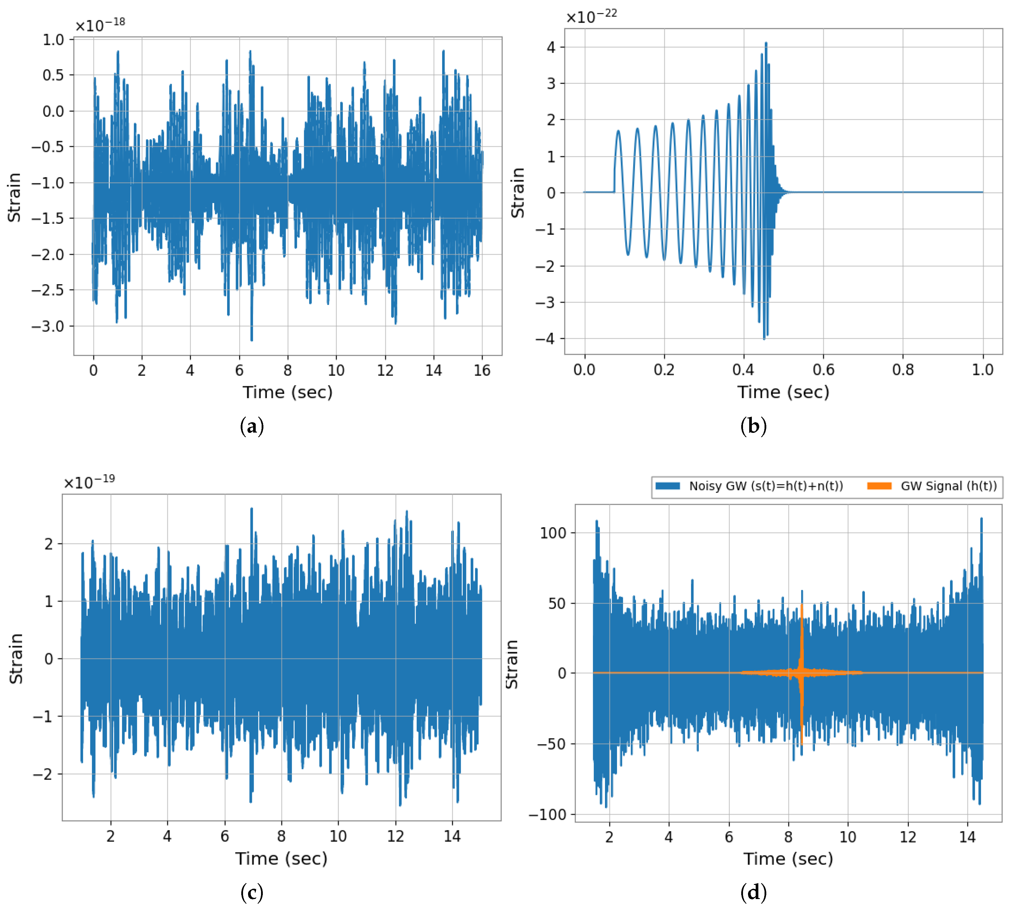
Figure 2. Time-series noise and GW data. (a) Real noise segment obtained from LIGO. (b) Simulated GW signal. (c) Filtered noise. (d) Filtered and whitened noisy GW signal and GW data with SNR = 8.18.
Electronics 14 04098 g002
Figure 3. One-second-long filtered and whitened noise and GW data with SNR = 8.18.
Electronics 14 04098 g003
Figure 4. Q-transform of injected signals for varying SNR values. (a) SNR = 8.41, (b) SNR = 9.93, (c) SNR = 16.87, and (d) SNR = 25.93.
Electronics 14 04098 g004
Figure 5. (a) ROC curve of the proposed EDAT-BBH model. (b) The 2D t-SNE projection.
Electronics 14 04098 g005
Figure 6. (a) A sample gravitational wave. (b) The Q-transform representation. (ce) DWT levels A, D1, and D2, respectively, and (f) energy mask constructed from both Q-transform and DWT-based energy to modulate attention.
Electronics 14 04098 g006
Figure 7. Attention maps from the four heads of the Transformer (ad) without masking (eh) and employing energy-based mask.
Electronics 14 04098 g007
Table 1. The hyperparameters used for the proposed model.
ParameterValue
Number of attention heads4
Number of attention layers2
Feedforward network size128
Dropout rate0.2
Learning rate 1 × 10 4
Input signal length2048
Number of patches224
Table 2. Performance of the models in terms of precision, recall, F1-score, accuracy, ROC AUC, and PR AUC.
ModelAccuracyPrecisionRecallF1-ScoreROC AUCPR AUC
Base Model [6]0.93150.97200.88850.92840.96790.9772
TFR–ResNet-101 [5]0.96950.99330.95530.96880.98810.9916
TFR–Xception [5]0.97040.99510.95870.96980.98810.9916
TFR–EfficientNet [5]0.97100.99450.95530.97030.98850.9920
EDAT-BBH0.99530.99560.99500.99530.99990.9998
Table 3. Performance of the proposed model and CoT models in terms of F1-score and AUC.
ModelF1-ScoreAUC
CoT-temporal [8]0.91400.9350
CoT-spectral [8]0.91600.9380
EDAT-BBH0.99530.9999
Table 4. Performance comparison of dual-energy fusion models with varying weighting factors.
MetricStat α = 1 α = 0.8 α = 0.2 α = 0 α = 0.5
(Only Q-Transform)(1 − α) = 0.2(1 − α) = 0.8(Only DWT)(1 − α) = 0.5
Accuracy (%)Mean99.1599.3699.3499.3299.53
Std0.680.230.320.150.09
Min97.9599.1098.7899.1099.45
Max99.6599.6099.5899.4899.63
CI Lower98.3099.0798.9499.1399.38
CI Upper99.9999.6599.7399.5099.68
PrecisionMean0.98820.99010.99110.99340.9956
Std0.01440.00570.00760.00490.0022
Min0.96330.98330.97750.98710.9925
Max0.99800.99700.99501.00000.9980
CI Lower0.97030.98300.98160.98400.9920
CI Upper1.00000.99721.00001.00000.9992
RecallMean0.99500.99720.99570.99290.9950
Std0.00400.00210.00220.00630.0024
Min0.98850.99450.99250.98200.9915
Max0.99900.99950.99850.99750.9975
CI Lower0.99010.99460.99300.98510.9920
CI Upper0.99990.99980.99841.00000.9988
F1-ScoreMean0.99150.99360.99340.99310.9953
Std0.00660.00230.00320.00150.0009
Min0.97990.99110.98790.99090.9945
Max0.99650.99600.99580.99470.9963
CI Lower0.98330.99080.98950.99120.9938
CI Upper0.99980.99650.99730.99500.9965
ROC AUCMean0.99980.99980.99970.99980.9999
Std0.00020.00020.00020.00010.0001
Min0.99950.99940.99950.99970.9998
Max0.99990.99990.99990.99990.9999
CI Lower0.99950.99950.99950.99970.9998
CI Upper1.00001.00000.99990.99991.0000
Table 5. Comparison of attention interpretability metrics with and without energy masking.
MetricNo Mask (Mean)Mask (Mean) Δ p-Value (Wilcoxon)
Attention-SNR corr−0.07780.3567+0.4345< 10 300
IoU0.03780.0519+0.0141 7.37 × 10 274
Entropy10.807110.7901−0.0169< 10 300
Table 6. Computational complexity and efficiency comparison of the proposed EDAT model (with and without energy masks) against standard CNN backbones.
ModelParams
(M)
FLOPs
(G)
Inference
(ms) (bs = 1)
Latency Std
(ms) (bs = 1)
Throughput
(samp/s) (bs = 1)
Inference
(ms) (bs = 32)
Latency
Std (ms) (bs = 32)
Throughput
(samp/s) (bs = 32)
ResNet10142.66015.195458.0128.762.254.50563.3240.7
Xception20.8649.134130.5202.777.624.24729.2989.9
EfficientNetB04.0510.800291.3486.253.429.45933.4271.1
EDAT (No Mask)0.2160.15441.5001.0123.85.3036.32417.7
EDAT (With Mask)0.2160.15442.1141.9323.53.8274.16512.6
Disclaimer/Publisher’s Note: The statements, opinions and data contained in all publications are solely those of the individual author(s) and contributor(s) and not of MDPI and/or the editor(s). MDPI and/or the editor(s) disclaim responsibility for any injury to people or property resulting from any ideas, methods, instructions or products referred to in the content.