A Comprehensive Radar-Based Berthing-Aid Dataset (R-BAD) and Onboard System for Safe Vessel Docking ^†

Abstract

Ship berthing operations are inherently challenging for maritime vessels, particularly within restricted port areas and under unfavorable weather conditions. Contrary to autonomous open-sea navigation, autonomous ship berthing remains a significant technological challenge for the maritime industry. Lidar and optical camera systems have been deployed as auxiliary tools to support informed berthing decisions; however, these sensing modalities are severely affected by weather and light conditions, respectively, while cameras in particular are inherently incapable of providing direct range measurements. In this paper, we introduce a comprehensive, Radar-Based Berthing-Aid Dataset (R-BAD), aimed to cultivate the development of safe berthing systems onboard ships. The proposed R-BAD dataset includes a large collection of Frequency-Modulated Continuous Wave (FMCW) radar data in point cloud format alongside timestamped and synced video footage. There are more than 69 h of recorded ship operations, and the dataset is freely accessible to the interested reader(s). We also propose an onboard support system for radar-aided vessel docking, which enables obstacle detection, clustering, tracking and classification during ferry berthing maneuvers. The proposed dataset covers all docking/undocking scenarios (arrivals, departures, port idle, and cruising operations) and was used to train various machine/deep learning models of substantial performance, showcasing its validity for further autonomous navigation systems development. The berthing-aid system is tested in real-world conditions onboard an operational Ro-Ro/Passenger Ship and demonstrated superior, weather-resilient, repeatable and robust performance in detection, tracking and classification tasks, demonstrating its technology readiness for integration into future autonomous berthing-aid systems.

1. Introduction

Berthing represents one of the most challenging phases in maritime vessel operations, demanding precise, deliberate and meticulously controlled maneuvering within confined and often intricate port environments. Its complexity is further intensified by adverse weather conditions, such as strong winds or low visibility, and intense maritime traffic. Vessels of all sizes predominantly depend on visual cues and crew observations to identify obstacles and support the captain during docking. Unfortunately, these visual approaches are highly susceptible to environmental conditions and prone to human error, resulting in miscalculations, faulty maneuvers and, in some cases, accidents [1]. In this respect, safe berthing remains a challenge for the maritime industry while currently available technologies lack the capacity to provide a robust foundation for autonomous ship berthing operations.

In this context, various sensor modalities may be considered for assisted berthing operations and, ultimately, autonomous ship berthing. Cameras are already employed perimetrically to ships, however adverse weather phenomena like fog, precipitation or low illumination significantly degrade the performance of camera-based observation systems thereby limiting their reliability in assisting safe docking [2]. Markedly, camera sensors inherently lack the capacity to directly measure object distances, thus further inhibiting their applicability. Lidar sensors may represent a powerful alternative for high-resolution obstacle detection and range measurement; however, they come with a hefty price tag while their performance is also compromised by adverse weather conditions [3,4]. Ferries typically rely on GPS and long-range radars for navigation. However, GPS is ineffective for docking due to its insufficient accuracy and refresh rate for close-range maneuvering [5], while long-range radars are designed for open-water navigation and lack the resolution and accuracy needed to detect nearby obstacles. Due to all these considerations and trade-offs, berthing operations are, even nowadays, almost entirely dependent on visual observation [1,2,5]—and this includes large vessels such as Ro-Ro/Passenger ferries and similar.

On the other hand, many studies have explored the use of radar-based tracking algorithms for improving maritime situational awareness [5,6], underpinning the applicability of radar-based obstacle detection systems in collision avoidance and real-time path planning. In contrast to long-range radar systems, low-power/short-range Frequency-Modulated Continuous Wave (FMCW) radars provide superior range resolution and may be particularly efficient in close quarters and challenging environments—such as those that are predominant during berthing. Indeed, there is recent evidence in the literature that microwave and millimeter wave radar sensors have the capacity to capture obstacles and objects within the harbor area [7]. From a commercial perspective, short-range FMCW radars, such as the ELVA-1 DR-76 for docking assistance and the SDM360-76 for situational awareness, demonstrate the role of high-resolution radar technology in supporting autonomous navigation [8,9]. However, both these technologies either focus on dock-installed systems [8] or collision avoidance in open waters [9], effectively leaving a significant research gap in short-range berthing assistance. Despite this gap, and in fact motivated precisely by it, we firmly believe that short-range, high-resolution FMCW radars will play a pivotal role in achieving the Maritime Autonomous Surface Ships (MASS) objective, which is highly praised within the maritime industry [5,6,10]. In this paper, we demonstrate the applicability of these radar sensors to (i) serve as a powerful complementary sensor modality for solutions specifically addressing ship berthing challenges, and (ii) accomplish this feat while being installed onboard ships, thereby ensuring unrestricted applicability in unknown ports and varying berthing conditions, especially in the absence of any assistance from port infrastructure, port operators, or smart port technologies.

In this context, we developed and presented a proof-of-concept radar-based berthing aid system, integrating multiple FMCW radar sensors at industrial and automotive frequency bands, alongside a camera sensor for synchronized and timestamped footage recording, as well as a variety of functionalities for autonomous operation [11]. Since then, the proposed platform underwent thorough testing in maritime environment, withstanding adverse weather conditions (extreme temperatures, marine saline humidity, storms, shocks and vibrations, etc.) over a two-month period onboard a Ro-Ro/Passenger ferry ship. The specific ship was by that period conducting frequent routes on an itinerary across 13 different island destinations in the Aegean Sea, Greece. Throughout this testing campaign, a comprehensive dataset comprising synchronized radar measurements and camera footage was systematically collected, covering all phases of docking and undocking procedures (arrivals at and departures from the port, idle periods within port, cruising during ramp on/off transition, etc.). The dataset, aptly named Radar-based Berthing-Aid Dataset (R-BAD), is herein presented in detail and has been made openly accessible online via Zenodo [12] to support further research and development within the marine automation and intelligent transportation systems communities.

Based on the herein proposed R-BAD dataset, and to further demonstrate its applicability, we processed the data in scenarios that emulate real-time operation, where radar-backscattered point-cloud data are clustered and targets are consistently tracked with superior performance, using, respectively, DBSCAN [13] and a Kalman filter [14] implementation of ours. On top of that, clustered radar data are annotated manually in two classes (dock/no-dock) using the camera footage for ground truth class designation. The annotated data are then employed to train several Machine-Learning (ML) models, namely Random Forest [15], XGBoost [16], PointNet [17], and Graph Neural Networks (GNNs) [18]. We consider that the dock is the main target class of interest for berthing; nevertheless, more classification models’ development is made feasible with the available dataset. All ML models performed substantially well, with GNNs achieving the highest classification performance and generalization across unseen ports.

In the following sections, the deployment of the proposed platform, the development of the R-BAD dataset, and the validation of our approach through DBSCAN, Kalman filtering and ML-models’ evaluation are presented.

2. Radar-Based Berthing Aid System

The proposed berthing aid system is composed of two main subsystems: a data acquisition subsystem responsible for collecting radar and video data, and a management and communication subsystem tasked with system control, connectivity and safety functionalities. The entire system is housed within a waterproof enclosure, specifically engineered for installation on the stern gunwale of the Ro-Ro/Passenger Vessel BS Patmos. A detailed overview of each subsystem is provided in the following subsections.

2.1. Radar and Video Acquisition Subsystem (RVAS)

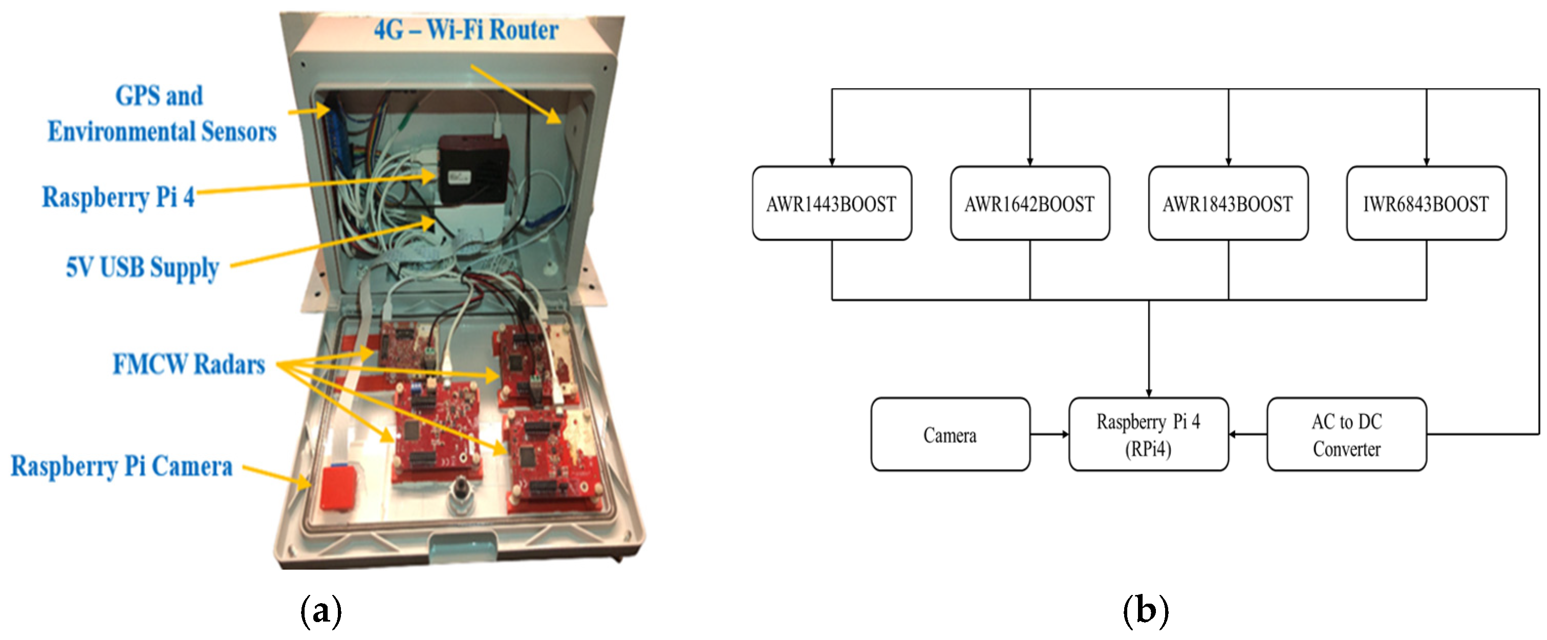
The Radar and Video Acquisition Subsystem (RVAS) consists of four FMCW radar sensors, namely the AWR1443BOOST, AWR1642BOOST, AWR1843BOOST, and IWR6843ISK. These devices operate across the 60–64 GHz (for the IWR6843ISK) and 77–81 GHz (for the remaining devices) frequency bands [19]. A Raspberry Pi 4 (RPi4) is employed as an edge processing and control unit. The RPi4 is tasked with the radar sensors’ functionality control and data acquisition and recording, while at the same time it is connected to a compatible camera for video footage capture—see Figure 1a for a photo of the proposed platform and its main modules, and Figure 1b for a block diagram of the RVAS. In Figure 1a specifically, it can be observed that the radar sensors are arranged in a way that their antenna array axes are vertical, and mounted on custom-designed, 3D-printed plastic supports, ensuring optimal dock targeting during port approaches.

The FMCW radar sensors are initially configured using the manufacturer’s (Texas Instruments, Dallas, TX, USA) Graphical User Interface (GUI), i.e., the web-based Visualizer application. The TI GUI generates corresponding configuration files (*.cfg) that contain all setup parameters for each sensor and completely specify the radar operating settings. During operation, different configuration files may be used to dynamically adjust the radar sensors’ setup according to specific measurement requirements, giving rise to scenarios like transitioning from long range and low resolution to close quarters and high range resolution measurements, simply by changing the employed cfg file. Additionally, the cfg files are directly editable and one is able to modify individual parameters, enabling the creation of custom configuration profiles tailored to the needs of each experimental scenario. This approach provides flexibility in sensor tuning and facilitates rapid reconfiguration of the radar system in response to varying environmental or operational conditions.

Following extensive measurement campaigns, we concluded to a set of radar parameters that provide an optimal balance between system performance and operational simplicity. These parameters, tabulated in

Table 1. Radar settings and parameters.

Radar Model	AWR1443	AWR1642	AWR1843	IWR6843
Frequency (GHz)	77–81	77–81	77–81	60–64
Number of Antennas	4Rx-3Tx	4Rx-2Tx	4Rx-3Tx	4Rx-3Tx
Mode	Detected points	Detected points	Detected points	Detected points
Frames per second	20	20	20	20
Clutter Removal	No	No	No	No
Range Resolution (m)	0.244	0.391	0.195	0.122
Max Unambigious range (m)	50	50	50	50
Radial velocity resolution (m/s)	0.13	0.13	0.13	0.11
Maximum radial velocity (m/s)	1	1	1	0.81
Azimuth resolution	15	15	15	15
CFAR threshold scale (0–100 dB)	15	15	17	12

for each radar sensor, were consistently applied in all experiments conducted as part of the herein presented Radar-based Berthing Aid Dataset (R-BAD) that is discussed in the next Section 3, Section 4 and Section 5. By standardizing the radar configuration across all measurement sessions, the experimental procedures described in this paper are repeatable and the resulting dataset maintains consistency in radar settings, ensuring simplicity and comparability of the collected data. Please also note that, according to the radar sensor specifications, the number of antennas used (entry “Number of Antennas”, Table 1) allows for angular output information at both the azimuth and elevation planes for the AWR1443, AWR1843 and IWR6843 sensors, and for the azimuth plane for the AWR1642 sensor.

The proposed platform, with the radar sensors set up according to the parameters of Table 1, was used to collect timestamped point clouds of detected radar targets. For each cloud point there is included its respective spatial information (x-y-z format), Doppler velocity, and signal-to-noise ratio (SNR). In parallel, video footage is synced, timestamped and recorded, using the provided RPi4-compatible camera. The R-BAD dataset collection procedure is discussed in detail in the next Section 3.

2.2. Management and Communications Subsystem (MCSS)

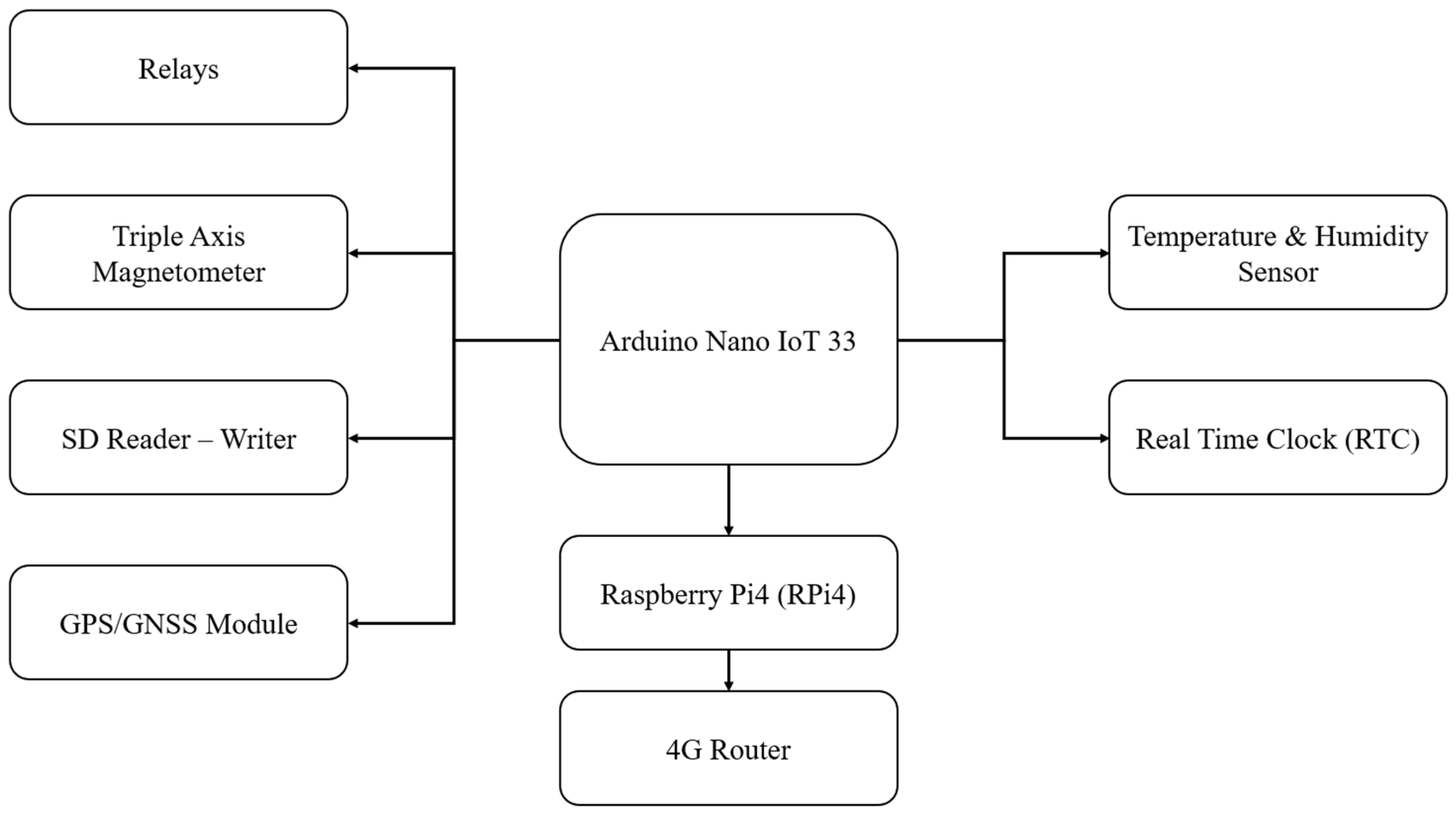
The Management and Communications Subsystem (MCSS) is responsible for managing power distribution, environmental monitoring, and wireless local and cloud communications. At the core of the MCSS is an Arduino Nano that is used to reliably control a series of critical environmental sensors (temperature and humidity), the GPS/GNSS module, a triaxial magnetometer, and a series of power relays. The MCSS is supervised by the RPi4 that also serves as an intermediate link with the RVAS. According to Figure 1a, the Arduino Nano is located above the GPS and environmental sensors and, at least in Figure 1a, it is hidden behind the enclosure’s brim. A connectivity diagram of the MCSS is provided by Figure 2 below.

The entire system is powered by the ferry’s AC power supply and AC/DC converters are used to provide reliable DC supply (see Figure 1b). However, power is distributed to subsystems via Arduino-controlled relays, as shown in Figure 2. The Arduino also controls a GPS sensor, temperature and humidity sensors, an accelerometer, a gyroscope and a magnetometer for vibration tracking, an RTC (Real-Time Clock) for timestamp synchronization, and an SD card reader/writer for local data logging. Furthermore, there is a SIM-based 4G router that provides cloud connectivity, enabling remote monitoring and telemetry. The MCSS logs environmental, timestamp, geo-location, inertial, etc., data, and encompasses various algorithms preserving safe operating conditions—e.g., if excessive temperature or humidity are observed, the MCSS automatically shuts down the system via the power control relays, in order to prevent further damage.

Additionally, by implementing geofences, the MCSS analyzes GPS coordinates to determine whether the vessel is within a port neighborhood. The Haversine method [20] is used to calculate the vessel-geofences distance and, when the geofenced boundary is crossed, the MCSS automatically activates the radar and video capture subsystem and logs data as berthing operations begin. It should be noted that the geofence boundaries are manually designated at a safe distance from the port to allow ample time for device boot-up and start of radar sensor logging before the dock enters the radars’ operational range.

Furthermore, the MCSS implements MQTT messaging, sending real-time status updates and sensor readings to the Cloud. Operators can also control the power of each component remotely, reboot the RPi4, start or terminate a measurement and monitor the device’s condition through a Telegram bot, allowing for flexible and remote management of system components.

2.3. System Deployment Onboard the BS Patmos Ro-Ro/Passenger Ferry Ship

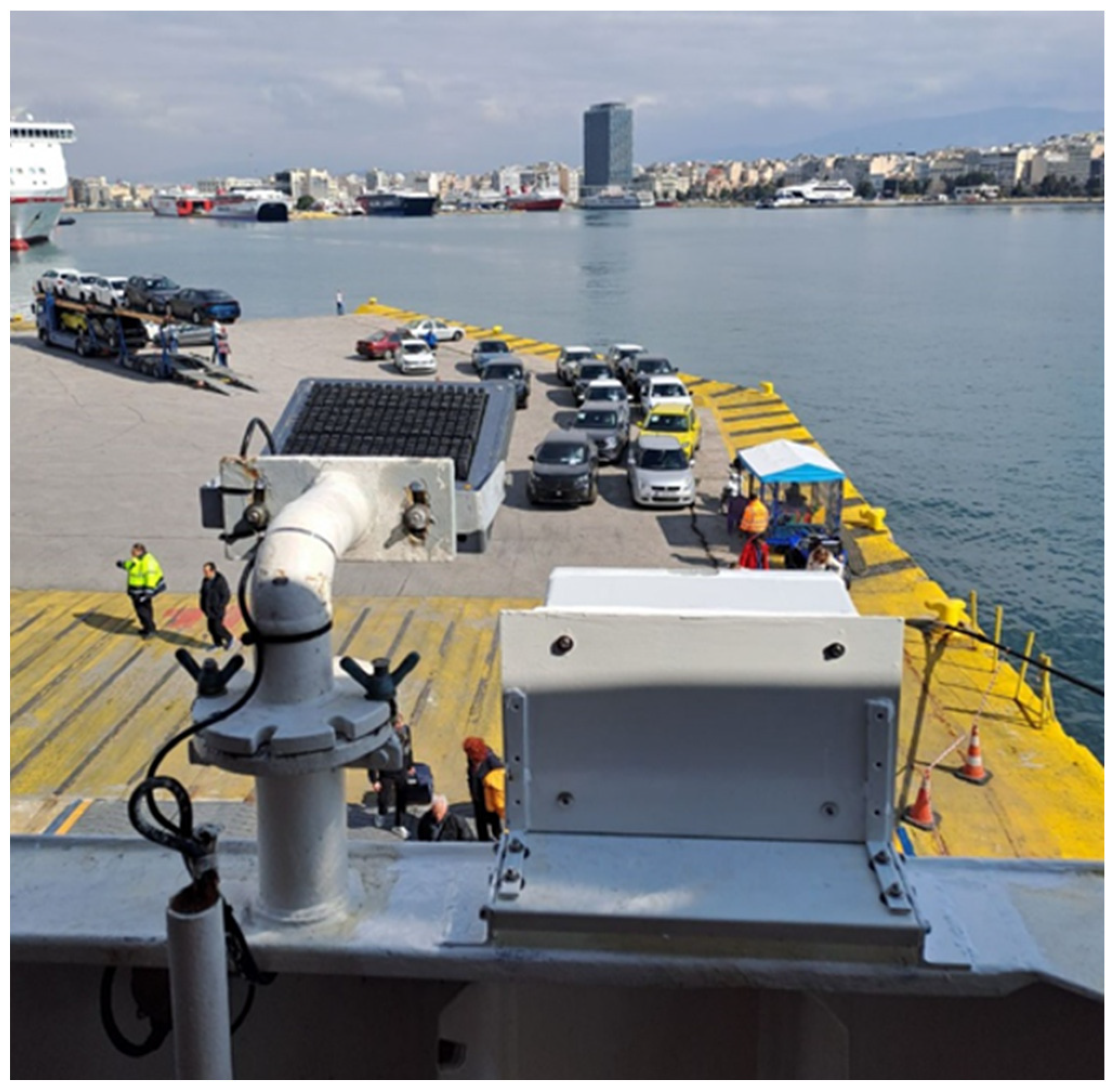
The proposed platform is deployed on the Ro-Ro/Passenger Ship BLUE STAR (BS) PATMOS of Attica Group S.A. group of companies. Mounted at the stern (Figure 3), the platform continuously monitors the vessel’s surroundings, identifying various obstacles such as the dock and nearby ships and vehicles. The deployment of our platform onboard a fully operational vessel allows for system testing in a real-life setting for a plethora of weather conditions and maneuvering complexities. Indeed, the route of the BS PATMOS consists of a total of 13 ports with different topologies and size, thus allowing for system testing in a large variety of port types, sizes, conditions, infrastructure etc.

Furthermore, it is noted that the system’s enclosure is engineered to withstand high vibrations, exposure to saltwater and high temperatures. It is securely mounted on a welded base attached to the gunwale of the vessel, ensuring stability while allowing for easy removal. Furthermore, marine-grade sealing is applied for durability in harsh conditions while thermal stress tests were conducted prior deployment emulating the highest operating temperature expected onboard. As previously mentioned, the proposed platform underwent thorough testing across a two-month period while the vessel BS Patmos was performing regular itineraries across 13 ports in the Aegean Sea in Greece. During this period, the platform was regularly inspected and no signs of degradation due to marine humidity or excess temperatures were observed. During this same two-month period, the RVAS was used to collect radar point cloud and video footage data, as mentioned in Section 2.1. In the following Section 3, a detailed discussion on the dataset collection is provided and followed by a dataset description immediately after.

3. Radar-Based Berthing Aid Dataset (R-BAD): Creation and Curation

The radar-based berthing aid system was deployed onboard the BS PATMOS ferry, as described in Section 2, and used to acquire the raw radar and video data forming the R-BAD dataset. Data acquisition was fully automated by means of GPS-based geofencing: when the vessel entered a predefined port boundary area, recording was initiated; data acquisition stopped after departure and upon exiting the aforementioned boundary. This ensured that only port-related sessions were captured.

The complete curation pipeline is illustrated in Figure 4 and consists of consecutive steps, from raw data acquisition to the final curated dataset. Each block in Figure 4 is described in the following subsections.

3.1. Data Collection

Four FMCW radar sensors (AWR1443, AWR1642, AWR1843, and IWR6843), from Texas Instruments (Dallas, TX, USA) operated concurrently at 20 frames per second, producing timestamped point clouds containing three-dimensional spatial coordinates (x, y, z), Doppler velocity, and signal-to-noise ratio (SNR). The onboard RPi4 managed data logging and stored radar outputs on local media, from where the complete dataset was subsequently retrieved for offline processing. A camera connected to the RPi4 simultaneously recorded video streams at 20 FPS. All recordings were timestamped using the RPi4 real-time clock (RTC), enabling subsequent alignment of radar and video streams during post-processing. Metadata such as session identifiers, start/stop times, and radar configurations were also recorded to support dataset organization and reproducibility.

3.2. Video Preprocessing

The captured video streams were stored in H.264 format by the onboard RPi4. For compatibility with standard playback and annotation tools, these streams were subsequently converted to MP4 format during post-processing on a host workstation. This step did not alter the content of the recordings but ensured ease of handling.

3.3. Data Organization per Port and Docking Attempt

To facilitate structured access, the recorded sessions were organized per port and docking attempt. The port label denotes the geographical location of each operation (e.g., Kalimnos, Patmos, Rhodes), while the docking attempt index reflects the sequential number of visits to the same port during dataset creation (e.g., Kalimnos_3 indicates the docking of the ship at the Kalimnos port, during a subsequent approach on a different date). This two-level hierarchy data organization enables both cross-port comparisons and intra-port analysis across multiple repetitions of similar maneuvers.

3.4. Data Quality Inspection

Each session underwent a quality control stage, verifying file integrity, completeness of timestamps, and consistency of frame counts between radar and video streams. Additional checks were performed to identify corrupt files, dropped radar frames, or video gaps. Sessions failing these checks were excluded or trimmed to retain only valid intervals.

3.5. Data Trimming and Alignment by Timestamps

The radar and camera sensors collected their data independently to one another, but their output frames carried timestamps from the RPi4 real-time clock (RTC). During post-processing, radar frames and video frames were matched using these timestamps. Frames within ±50 ms were considered to correspond to the same timeslot, while unpaired frames at the start or end of each sequence were excluded. This procedure ensured that radar and video sequences could be reviewed together on a consistent timeline.

3.6. Data Grouping per Docking Stage

Each session was partitioned into five docking stages: Arrival, Departure, Port-Idle, Cruising-Ramp Opening, and Cruising-Ramp Closing. This partitioning criterion is two-fold: on the one hand, each stage represents a different operational situation with different requirements for crew alertness, safety concerns and available reaction time in case of emergency. On the other hand, different docking stages correspond to different radar environments. More specifically, it is common practice for ferry companies to open and close the ferry ramp during the final moments before docking or the first moments following detachment from the dock, respectively. This ramp open/close routine severely alters the data and video sensor data and is herein considered a major criterion for data partitioning.

The boundaries between the aforementioned five docking stages were determined manually by inspecting the video recordings and identifying the exact transition moments (e.g., when the vessel begins maneuvering towards the dock, or when the ramp was opening/closing). This grouping enables stage-specific analysis of radar behavior under distinct operational conditions.

3.7. Data Filtering and Denoising

Filtering was applied to remove unreliable radar detections. Radar point cloud records falling out of predefined limits were discarded for clarity. Coupling artefacts—false detections appearing near the radar transmit-receive antennas due to transmitter–receiver direct coupling—were eliminated by removing all detected points that are closer than 3 m away from the radar transmitter and receiver antennas. These steps reduced noise and data clutter, and ensured that only meaningful detections were retained for subsequent processing. Please note that no interference between different co-located radar sensors was observed during our experiments.

3.8. Frame Aggregation and Unified Data Frame Creation

After filtering, detections from all radars recorded at the same timestamp were merged into a single Multi-Radar frame (MRF). Each MRF contains the spatial coordinates, Doppler velocity, and SNR values of all detections across all radars. This standardized representation forms the basis for subsequent clustering, tracking, and machine learning tasks.

4. Dataset

The proposed R-BAD dataset contains a total of 661 individual recordings, corresponding to approximately 69 h (4140 min) of synchronized radar and video data collected over more than four weeks on board a passenger roll-on/roll-off (Ro-Ro) ferry. The dataset has a total volume of 63.3 GB, of which 439 MB corresponds to structured CSV files containing sensor annotations and metadata, while the remaining files consist of the video recordings. Each recording has an average duration of about 35 min, and to facilitate analysis, the dataset is divided into five main categories representing distinct operational states of the vessel:

• Arrival: Recordings capturing the vessel’s approach to port, typically lasting around 4 min, where docking maneuvers and reduced speeds dominate.
• Cruising-Ramp Closing: Recordings of the vessel cruising just before arrival, during which the stern ramp is unlocked and prepared for docking, with similar duration statistics to ramp closing.
• Port-Idle: The longest category, covering idle periods while the vessel remains stationary at the port, typically lasting more than 13 min per recording. This category corresponds to passengers and cars hopping out of and into the ship.
• Cruising–Ramp Opening: Data recorded shortly after departure, when the vessel is starting to speed up and the stern ramp is in the process of being secured, averaging about 4.5 min per recording.
• Departure: Recordings covering the vessel’s maneuvering away from port and accelerating to open water, with shorter mean duration of about 2.5 min

For each of these categories,

Table 2. Dataset volume and duration per category.

Category	Recordings	Total Duration	Mean Duration	Rows	Volume (GB)	Mean Volume (GB)
Arrival	123	8.46 h or 508 min	4:04	609,100	~7.7	0.06
Cruising–Ramp closing	129	9.91 h or 595 min	4:37	713,380	~9.3	0.07
Cruising–Ramp opening	146	10.79 h or 647 min	4:26	774,300	~10.4	0.07
Departure	122	5.57 h or 334 min	2:35	379,580	~5.5	0.04
Port–Idle	139	31.2 h or 1872 min	13:28	2,247,560	~3.6	0.21
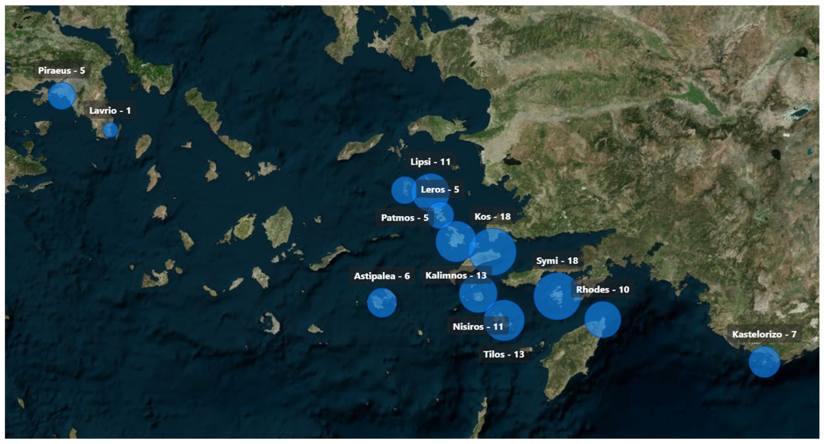
Total	661	69 h or 4140 min	5:50	4,723,920	~36,5	0.09

summarizes the number of recordings, the total and mean duration, the number of annotated rows in the CSV files, the overall data volume, and the average file size. Among them, the most critical for analysis is the Arrival category, since it represents the most critical docking stage in terms of operational alertness, safety concerns, reaction time available to the crew due to the ship being in close quarters to the dock, etc. This category will be the primary focus in the next section and will be used for the classification of the dock. The remaining categories are provided in the aforementioned open-source R-BAD dataset with the aim of inspiring researchers to use them for their own projects, clustering, tracking and classification techniques development, etc. Having said that, the Arrival category has an average measurement duration of 4 min and 30,480 annotated rows and corresponds to 123 recordings from 13 different ports (see Table 2); these ports are mainly located in the Southeast Aegean Sea and the wider Attica regions, as illustrated in Figure 5.

4.1. Dataset Composition and Recording Statistics

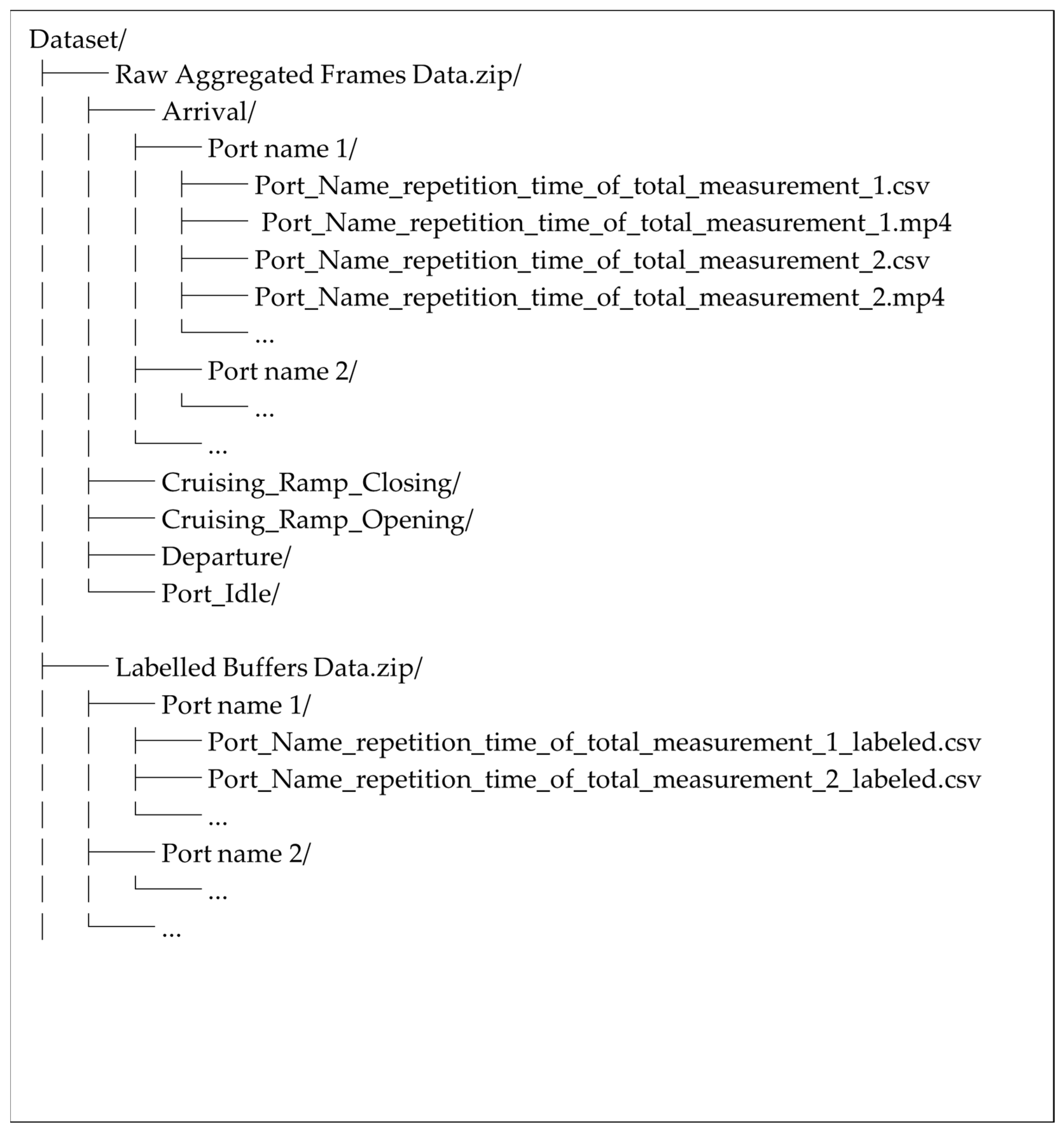
The dataset is organized into two main folders, namely “Raw Aggregated Frames Data” and “Labelled Buffers Data”. The former is divided into five operational categories (Arrival, Cruising–Ramp Closing, Port–Idle, Cruising–Ramp Opening, and Departure)—as described in Table 2. Within each category, the recordings are further divided based on the port where they were collected, resulting in 13 port-specific subfolders. Each subfolder contains pairs of files for every recording, i.e., (i) a Comma-Separated Values (CSV) file with structured Raw Aggregated Frames Data from each radar, including timestamps, radar detections and vessel operational states, and (ii) the corresponding synchronized video in MP4 format. This organization is consistent across the dataset. As long as the “Labelled Buffers Data” main folder is concerned, it further contains an extra folder that includes the data category classes following the same aforementioned hierarchy. Furthermore, the folder “Labelled Buffers Data” does not contain any video files since they are already available in the unlabeled dataset. A visual representation of the hierarchy is shown in Figure 6 below.

Focusing again on the “Raw Aggregated Frames Data” folder, the unlabeled CSV files contain the preprocessed radar data, where ‘preprocessed’ refers to the steps described in Section 3 and illustrated in Figure 4. Each CSV includes the frame number, the POSIX timestamp, and the radar measurements in the form of [X, Y, Z, Velocity, SNR] for every MRF detection captured by each radar. Again, for readability, MRF stands for Multi-Radar Frame, see Section 3.8.

On the other hand, the annotated (labeled) data undergoes an additional preprocessing step, described in detail in Section 5, which results in a different internal structure compared to the unlabeled CSVs. As an example, please refer to

Table 3. Snippet from labelled csv “log_Tilos_2_05_09-09_29_labeled”.

Time	Frame_ID	Tracking_ID	X	Y	Z	Num_Points	Points	Label
0:02	59	1	−1.96	12.98	2.22	41	[…]	0
0:04	99	2	−3.43	7.86	0.61	63	[…]	0
0:04	99	3	−1.87	13.04	2.05	31	[…]	0
0:05	119	2	−3.45	7.85	0.86	102	[…]	0
0:05	119	3	−1.9	13.01	2.25	39	[…]	0
0:06	139	2	−3.44	7.82	1.13	44	[…]	0

below, which depicts the first six rows of the CSV file “log_Tilos_2_05_09-09_29_labeled” that contains the labeled data for the 2nd arrival at the port of Tilos.

In this format, the time column no longer follows the POSIX standard but instead represents the elapsed duration from the beginning to the end of the recording. The Frame_ID is defined at a reduced rate by aggregating every 20 MRFs (Multi-Radar Frames, see Section 3.8), thereby forming what we define as a Multi-Radar Sequence (MRS). Consequently, each Frame_ID corresponds to the last MRF within its respective MRS. As will be described in detail in Section 5, each aggregated MRF undergoes a clustering post-process step, resulting in a cluster Tracking_ID for each MRS. This Tracking_ID is assigned to each detected cluster and maintained across MRSs, providing a unique identifier for temporal tracking. The spatial features (X, Y, Z) correspond to the centroid of each cluster in three-dimensional space, while the Num_Points field indicates the number of radar detections that contributed to forming the cluster. The corresponding Points entry contains the list of raw radar measurements [X, Y, Z, Velocity, SNR] used to generate the cluster.

Finally, the Dock label column provides the manual annotation of the vessel’s operational state, distinguishing between dock and no-dock conditions. An example is shown in Table 3, with extra caution on the fact that there can be multiple rows with the same Time and Frame_ID column due to the presence of different clusters.

4.2. Explaratory Data Analysis

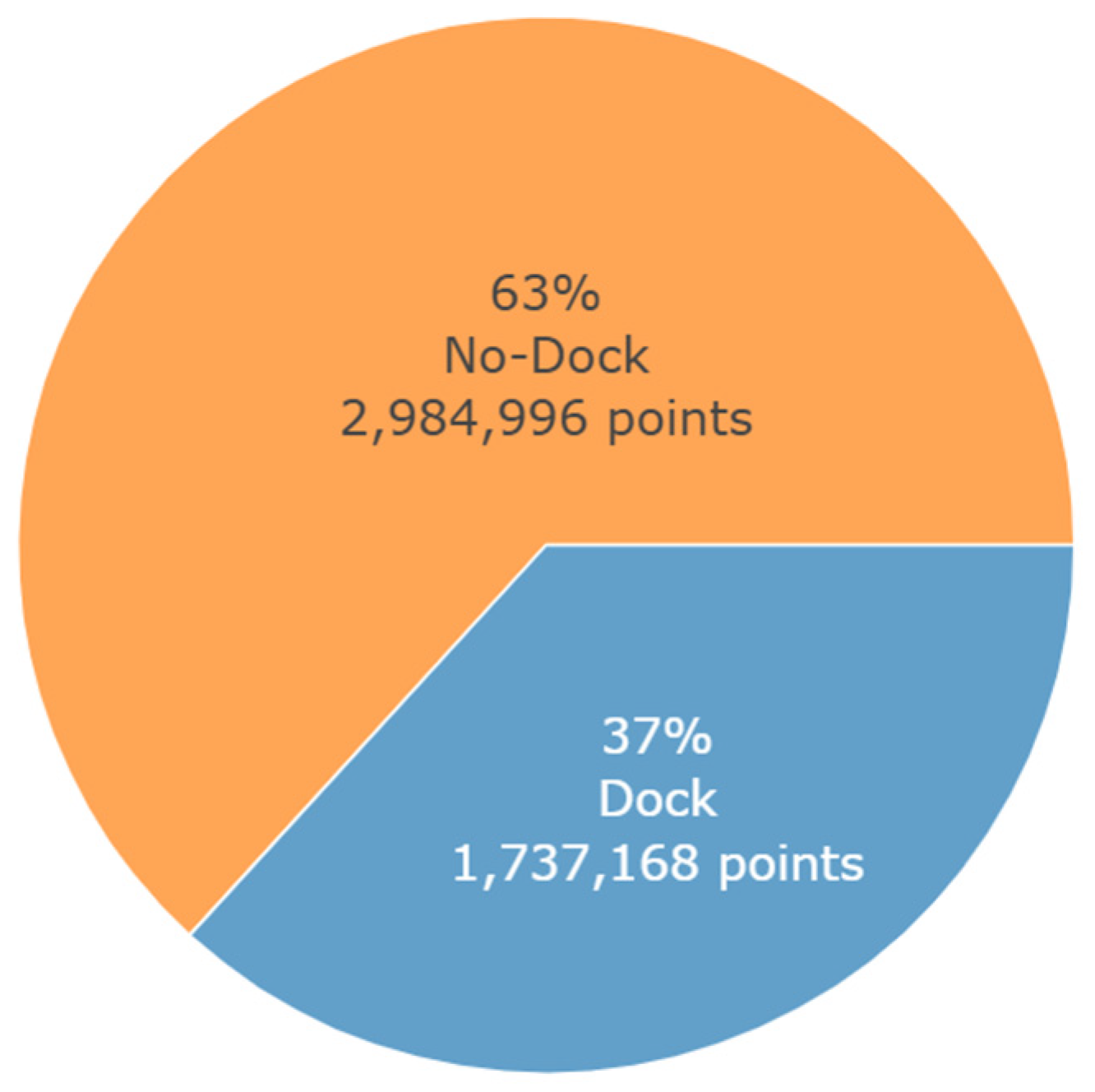
Out of all data categories (Arrival, Cruising–Ramp Closing, Port–Idle, Cruising–Ramp Opening, and Departure), it is considered the Arrival subsection is the most crucial for navigation safety in close quarters, and this is the one that we further focus our analysis on. In this context, we herein also provide a detailed analysis for a better understanding of its content. More specifically, the Arrival category consists of 123 recordings that consist of 508 min and 609,100 rows of data in total, containing a total of 4,722,164 points. Of these, 1,737,168 points correspond to the Dock, while the remaining 2,984,996 points represent noise and other objects that are not traceable. The imbalance in the distribution of points can be seen in Figure 7, where the Dock accounts for 37% of the total points, while the remaining 63% correspond to other, non-traceable elements. This distribution reveals that the two classes occupy different proportions of the total recording time, which is expected since, throughout all arrivals, the Dock class appears for only a relatively short portion of each sequence. This imbalance reflects the dynamics of the berthing process: for most of the duration, the radar primarily detects transient elements such as the ferry ramp, vehicles, or miscellaneous dockside objects, whereas the actual dock is observed for a much shorter period.

Another perspective on the dataset is to examine the relative contribution of each radar to the overall number of detections, irrespective of whether a point corresponds to the dock, noise, or other reflections. As shown in Figure 8 both the absolute counts and percentages of points are reported, summing to a total of 6,649,607 detections. A notable observation is that the AWR1443 alone contributed more than 62% of the points, while the other radars contributed substantially fewer detections. This imbalance is not an artifact of the environment but is primarily due to the different CFAR configurations applied on each radar during data collection (Table 1). In particular, although all devices used similar window, guard, and noise averaging parameters, the AWR1443 was configured with a lower CFAR threshold scale (15 on a 0–100 dB scale), resulting in significantly more detections being reported compared to the other radars. These settings were deliberately selected to ensure stable operation of all devices, as during initial trials some radars experienced processing crashes under heavy loads (many detected objects in one frame).

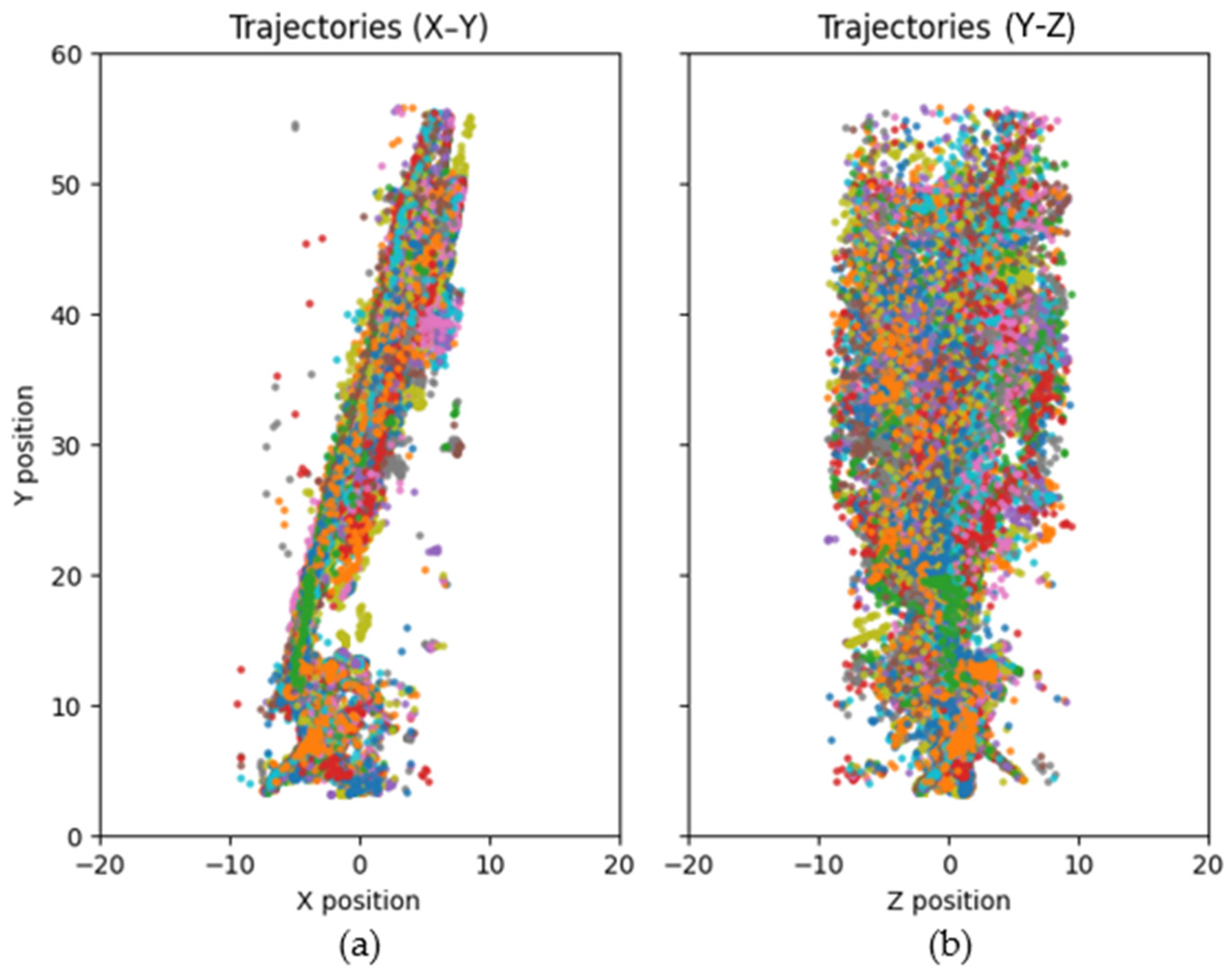
Lastly, examining the trajectories of the centroids provides valuable insights into the vessel’s movement patterns and helps to better understand the maneuvers most frequently performed by the captain during the berthing stage. As an example, Figure 9 depicts the trajectories of the dock centroids, over all labelled data, in the X-Y and Z-Y planes (Figure 9a,b). More specifically, the Y-axis is the direction of max radar antenna radiation while the X-axis is perpendicular to the Y-axis and faces upwards. Then, the Z-axis is perpendicular to both the X and Y-axes, colinear to the left-right axis of the ship, and faces towards the right as one observes the ship from its stern. It follows that the X-Y plane is the side view of the ship and dock scene, while the Z-Y plane is the corresponding top view and parallel to the sea level.

By observation of the X-Y plane, it follows that the apparent dock elevation is reduced as the ship approaches the dock. This is expected since the radar sensors were mounted with an inclination angle of 12° as discussed in Section 2 (see also Figure 1 and Figure 3). On the other hand, the Y–Z plane is a top view of the scene, and one may observe that the trajectories are randomly distributed across the scanned area, capturing a wide variety of ship approach paths. It follows that the proposed dataset includes a comprehensive range of berthing maneuvers, covering different approach angles and docking trajectories, which reflect a realistic operational variability.

To ensure a realistic and robust evaluation of the models’ ability to generalize to unseen environments, the dataset was split in two different ways (Split #1 and Split #2), each with a different combination of ports in their training, validation, and test subsets, as shown in

Table 4. Dataset Splits per Set Type.

Set Type	Split #1	Split #2
Training (65%, 62%)	Kalimnos (13), Kastelorizo (7), Lipsi (11), Nisiros (11), Patmos (5), Piraeus (5), Rhodes (10), Symi (18)	Astipalea (6), Leros (5), Kalimnos (13), Lipsi (11), Patmos (5), Piraeus (5), Symi (18), Tilos (13)
Validation (24%, 20%)	Astipalea (6), Kos (18), Leros (5)	Kos (18), Kastelorizo (7)
Test (11%, 18%)	Lavrio (1), Tilos (13)	Lavrio (1), Rhodes (10), Nisiros (11)

. In Split #1, the measurements were divided into 65% training, 24% validation, and 11% test, while in Split #2 they were divided into 62% training, 20% validation, and 18% test. In both splits, no port appears in more than one set, so that evaluation reflects generalization to completely unseen port environments. By rotating the port assignments across different splits and ensuring no overlap in test locations, this methodology provides a stronger assessment of generalization performance than a single static split would allow.

Although the Leave-One-Scene-Out (LOSO) strategy is commonly used to enforce strict separation between training and test data and to test all possible combinations, it was not adopted herein due to the high variability in the number of measurements per port. Some locations, such as Lavrio, were represented by only a single measurement, while others, such as Kos or Symi, are represented by many. This imbalance would produce unstable folds and unrepresentative test results in LOSO evaluation, especially when single-measurement ports dominate the test set. The two predefined splits instead provide a more balanced and interpretable benchmark, while still respecting strict port-level independence.

5. Clustering, Tracking and Annotation

5.1. Data Clustering with DBSCAN

As is analytically described in Section 3, in particular Section 3.8., radar detected point clouds from all sensors are aggregated into MRFs. The detections within each MRF are clustered using the DBSCAN algorithm (Density-Based Spatial Clustering of Applications with Noise) [13]. It is a method of unsupervised machine learning that categorizes the points into three groups: core points, border points and noise or outliers. DBSCAN creates clusters based on two main parameters, the first one is ε (epsilon) that defines a radius around each point, and the second is “minimum points” that refers to the minimum number of points (where points are the detections from the radars) that should exist within the radius ε in order for a cluster to be formed [21]. Core points are the points that have at least minimum number of points in radius ε, border points lie within the ε-neighborhood of a core point but do not fulfill the minimum number of points to be considered core points and last noise or outliers are the points that do not belong to any cluster. Twenty consecutive MRFs (corresponding to one second of data) are aggregated to form a Multi-Radar Sequence (MRS), as described in Section 4.2. Subsequently, the points of each MRS are clustered using DBSCAN with empirically tuned parameters, of ε-neighborhood radius set at 3 m and a minimum of 20 points per cluster. These settings allow the exclusion of sparse or noisy detections while retaining coherent physical structures, such as dock surfaces or prominent ship structures. Each identified cluster is characterized by its centroid coordinates (X, Y, Z), the number of associated points, X, Y, Z coordinates for each associated point as well as Doppler velocity, and Signal-to-Noise Ratio (SNR) for each one point as well.

5.2. Kalman Filtering for Cluster Tracking

To ensure consistent cluster tracking across consecutive MRSs and assign unique IDs to each detected cluster, a multi-object Kalman filtering approach is implemented. The Kalman Filter is a mathematical tool used to estimate a system’s variables that cannot be directly measured or are not available in the data [22]. It consists of a set of recursive equations that provide an efficient computational implementation of the least-squares method, enabling the estimation of past, present and future states of a system when an exact analytical model is not available [23]. Initially the filter was applied to linear systems or linear approximations of systems. Later the EKF (Extended Kalman Filter) or Schmidt Filter was introduced to handle non-linear systems by applying linear approximations through partial derivatives [24].

Herein, we closely follow the methodology and steps of a Kalman filter as described in [25]. The initial state vector of the system contains the x, y, z coordinates of each cluster at timeslot n as well as the differences dx, dy, dz between the coordinates of the same cluster for timeslots n and n − 1 (remember that, for a time interval between consecutive MRSs set to 1 s, this corresponds to the initial velocity of each cluster). With each following step, a subsequent state vector is predicted and the Kalman gain is recalculated using a new measurement. Finally, the error covariance is updated at each step to incorporate each new measurement to each subsequent prediction step, respectively.

The purpose of employing Kalman filtering was to enhance cluster tracking continuity between MRSs rather than refining position accuracy. Each cluster initiates a separate Kalman filter, maintaining a 6-dimensional state vector representing position and velocity. During tracking, newly detected clusters are matched to existing Kalman tracks using a nearest-neighbor approach with a distance threshold. For each predicted track position, the Euclidean distance to all detected cluster centroids is computed. If the closest centroid falls within a 5 m radius, it is assigned to that track and used to update the Kalman filter. When no detection is found within the threshold, the track continues only with its predicted position; if this situation persists for one MRS, the track is terminated. Any detection that cannot be linked to an existing track starts a new Kalman filter with a unique ID.

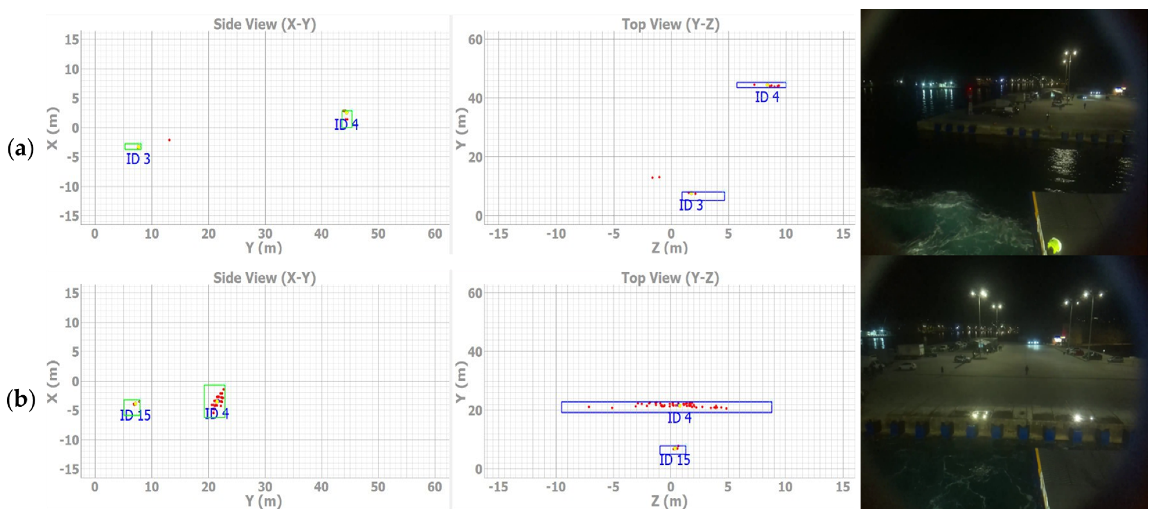
Figure 10 illustrates the combined visualization of radar-based clustering and tracking alongside synchronized camera footage during two distinct timeslots within a berthing maneuver. In the radar plots, red dots represent the raw radar detections, while green and blue rectangles indicate clusters identified by DBSCAN and tracked by Kalman filtering. The subplots provide two perspectives of the same detections: the side view (X–Y plane) shows the lateral spread of points along the berth, while the top view (Y–Z plane) projects the detections as seen from above, revealing their distance from the radar and their vertical distribution.

In Figure 10a, the corresponding dock-vessel distance is approximately 42 m and the dock is already identified as a stable cluster (ID4) and consistently tracked across views. In Figure 10b, at a closer distance of 22 m, the density of radar detections increases, allowing the dock’s shape to be defined more accurately, while the Kalman filter maintains continuity of the same cluster ID. The camera snapshots on the right provide the corresponding visual confirmation, validating the radar-based clustering and tracking performance.

5.3. Clustering and Tracking Performance Evaluation

The performance of the clustering and tracking processes was validated by assessing the consistency of cluster formation and the stability of tracking identifiers across successive buffers. DBSCAN was used to cluster radar detections with the aim of identifying the dock and differentiating it from other objects such as nearby ships, vehicles, or pedestrians. Validation of the clustering stage was performed through the herein-defined metric dbscan_correct, which measures the percentage of buffers in which DBSCAN successfully identified the dock as a distinct cluster.

To maintain cluster identity over time, Kalman filtering was applied to track cluster centroids across consecutive buffers. Each detected cluster was assigned a unique tracking ID, and the Kalman filter predicted its position in the next buffer. Validation of tracking stability was performed via the herein-defined metric kalman_changes, which counts the number of unnecessary ID reassignments. The corresponding stability percentage was calculated as the inverse, i.e., the proportion of buffers where IDs remained consistent.

As an example, regarding the performance evaluation of the proposed clustering and Kalman filtering pipelines,

Table 5. Validation of Clustering & Tracking for 2 Ports.

	MRS = 20 Frames		MRS = 10 Frames
	Port of Kos	Port of Kalymnos	Port of Kos	Port of Kalymnos
$\mathrm{S}\mathrm{u}\mathrm{c}\mathrm{c}\mathrm{e}\mathrm{s}\mathrm{s}\mathrm{f}\mathrm{u}\mathrm{l} \mathrm{D}\mathrm{o}\mathrm{c}\mathrm{k} \mathrm{C}\mathrm{l}\mathrm{u}\mathrm{s}\mathrm{t}\mathrm{e}\mathrm{r}\mathrm{i}\mathrm{n}\mathrm{g}\left(\%\right)$ $=100 \ast {\displaystyle \frac{dbscan\_correct}{total\_buffers}}$	99.07	86.99	92.26	81.60
$Kalman Tracking Stability \left(\%\right)$ $=100 \ast \left(1-{\displaystyle \frac{kalman\_changes}{total\_buffers}}\right)$	97.66	86.18	86.87	70.40

provides numerical results for the ports of Kos and Kalymnos. More specifically, DBSCAN successfully clustered the dock in over 99% of buffers in the port of Kos and in approximately 87% in the port of Kalymnos, while Kalman filtering maintained stable tracking IDs in 97.7% and 86.2% of buffers, respectively. These results confirm the robustness of the proposed pipeline in ensuring both reliable dock clustering and continuous tracking, even in scenarios with temporary occlusions or noisy detections.

To determine the optimal size of the MRS (reminding an MRS is defined earlier as a Multi Radar Sequence), additional experiments were conducted using a shorter MRS of 10 MRFs (0.5 s) instead of the original 20 MRFs (1 s). For the port of Kos, the DBSCAN and Kalman filtering performance decreased to 92.76% and 86.87%, respectively, while for the port of Kalymnos the corresponding values were 81.60% and 70.40%. These values are significantly lower than those achieved with the 20-frame MRS (Kos: 99.07% and 97.66%; Kalymnos: 86.99% and 86.18%), highlighting the stabilizing effect of aggregating a full second of radar detections. However, increasing the MRS length beyond one second was not considered practical, as it would compromise the refresh rate required for real-time docking assistance. Therefore, the choice of a 20-frame MRS provides an appropriate balance between temporal smoothing and operational responsiveness.

5.4. Cluster Annotation

Labeling was performed on a per buffer basis. To facilitate this process, a custom Python-based graphical user interface (GUI) developed in Python 3.10 was used. This tool enabled annotators to simultaneously inspect the radar cluster positions and their associated video frames, ensuring a synchronized and intuitive labeling environment. The GUI supported quick navigation between MRSs, overlaid cluster visualization, and automated preloading of video segments aligned with radar timestamps, significantly reducing workload.

The primary labeling criterion was the spatial relation of each cluster to the dock infrastructure, as seen in the synchronized video stream. Clusters associated with dock surfaces were labeled as “Dock” (label = 1), while all others—including reflections from the sea, other vessels, cars, people and background objects—were labeled as “No Dock” (label = 0).

The final annotated dataset was stored in structured CSV files, with each row representing a tracked cluster. For every cluster, the CSV includes its Frame_ID, Tracking_ID, centroid coordinates (X, Y, Z), the number of associated points, and the assigned label. In addition, a dedicated field stores the full list of per-point detections, where each point is described by its own X, Y, Z coordinates together with Doppler velocity and SNR values. An example excerpt of such an annotated CSV file is shown in Table 3. This annotated dataset serves as the ground truth for training and evaluating supervised machine learning models for automatic dock detection, and it provides a robust basis for benchmarking detection and classification performance across diverse berthing scenarios.

As part of the annotation procedure, individual radar detections that did not belong to any DBSCAN-formed cluster were intentionally discarded and not logged into the CSV. The purpose of this was to eliminate noise and retain only coherent and physically meaningful clusters. Therefore, the DBSCAN parameters were tuned to reliably filter out noise while retaining valid dock-related clusters.

6. Dock Classification Models and Results

To further investigate the applicability of the proposed R-BAD dataset, we hereby employ a variety of machine learning techniques for the classification of radar point clouds as either “Dock” or “No Dock.” The models employed in this work include Graph Neural Networks (GNNs), PointNet, XGBoost, and Random Forest, each chosen for its distinct characteristics in handling spatial radar data.

6.1. Engineered Features

For the feature-based models, a diverse set of engineered features was extracted from each radar cluster to capture its statistical, spatial, and temporal characteristics. The goal of this step is to convert the irregular, unstructured nature of radar point clouds into meaningful information about the underlying geometry and signal properties of the detected objects. The selected features fall into four main groups:

6.1.1. Correlation Metrics

We computed the Pearson correlation between Doppler velocity and SNR values within each cluster, quantifying whether strong reflections tend to co-occur with particular motion patterns. In addition, the entropy of the Doppler and SNR distributions was calculated to capture the degree of variability and uncertainty in these measurements.

6.1.2. Eigenvalue-Based Geometric Descriptors

After mean-centering each cluster, we formed the 3 × 3 covariance matrix of point coordinates and extracted its eigenvalues (λ₁ ≥ λ₂ ≥ λ₃). From these, standard shape features were derived: linearity = (λ₁ − λ₂)/λ₁, planarity = (λ₂ − λ₃)/λ₁, sphericity = λ₃/λ₁, and elongation = 1 − λ₂/λ₁, along with eigenvalue ratios (λ₁/λ₂ and λ₂/λ₃). These features capture whether a cluster is elongated, surface-like, spherical, or compact, which is critical for distinguishing dock returns from clutter.

6.1.3. Dimensional Characteristics

Several size- and density-related features were computed, including cluster compactness (mean distance of points from centroid), bounding-box volume, density (points per unit volume), and average distance to centroid. Docks tend to produce compact, high-density, planar clusters, whereas water or wakes appear more diffuse and less structured.

6.1.4. Temporal Differences

To exploit dynamics across frames, clusters identified by the same tracking ID were compared sequentially. For each frame-to-frame pair we calculated displacements (ΔX, ΔY, ΔZ), speed, and velocity angle, as well as changes (Δ) in all scalar features (e.g., Δmean SNR, Δdoppler range, Δeigenvalues). These temporal features highlight stability for stationary structures such as docks and variability for moving clutter or noise.

Together, these engineered features provide a rich statistical and geometrical representation of radar clusters, enabling traditional classifiers such as Random Forest and XGBoost to robustly separate “Dock” from “No Dock” categories.

6.2. Evaluation Methodology

To assess the performance of the classification models, we used standard classification metrics: precision, recall, and F1-score. Precision quantifies how many of the predicted positives are actually correct, which is essential for minimizing false alarms. Recall measures the proportion of actual positive samples that were correctly identified by the model, indicating its ability to capture relevant cases. F1-score is the harmonic mean of precision and recall and provides a single, balanced metric that is particularly useful in scenarios where the dataset is imbalanced or where both false positives and false negatives carry significant weight.

In particular, F1-score is used as the primary metric for evaluating model performance, as it effectively reflects the trade-off between false positives and false negatives across the two classification categories: “Dock” and “No Dock.” For a more comprehensive understanding of model behavior, confusion matrices are also presented for each evaluation set to help validate the accuracy of the predictions but also the robustness and generalizability of each model across different port environments.

6.3. Random Forest-Based Classification Model and Results

6.3.1. Random Forest Model Architecture

Random Forest, an ensemble learning method based on decision trees, was used to handle the radar data’s structured features. The model was trained on the set of engineered features discussed in Section 6.1. The ensemble consisted of 200 decision trees, using class-balanced weighting to address slight class imbalance. Parallel training (n_jobs = −1) was employed to reduce training time, and a fixed random seed (random_state = 42) ensured reproducibility.

6.3.2. Random Forest Model Results

Despite its simplicity compared to neural architectures, the Random Forest model demonstrated strong classification performance, particularly in the “No Dock” class. When evaluated on the Split #1 test set, it achieved an F1-score of 95.7% for “No Dock” and 92.0% for “Dock”, indicating balanced performance across both categories. Notably, precision for “Dock” reached 97.1%, reflecting the model’s low false positive rate, while recall was lower at 87.5%, suggesting occasional missed dock detections. The inverse trend was observed in the “No Dock” class, where recall was high at 98.5%, and precision slightly lower at 93.0%, indicating a tendency to occasionally misclassify dock points as background.

Moving on to Split #2, which includes an entirely different split of ports for training and evaluation, the model preserved strong performance, though with a slightly different error profile. In this case, precision for the “Dock” class remained high at 95.4%, but recall dropped to 83.2%, leading to a slightly reduced F1-score of 88.9%. This shows that while the model remained conservative in predicting “Dock” (avoiding false positives), it became more prone to false negatives when applied to previously unseen environments. For “No Dock,” performance was also strong, with recall of 97.8% and F1-score of 94.5%, although precision was slightly lower at 91.4%.

These results are summarized in the following

Table 6. Results of Random Forest model for Split #1 and Split #2.

	Split #1		Split #2
	Dock	No-Dock	Dock	No-Dock
Precision (%)	97.1	93.0	95.4	91.4
Recall (%)	87.5	98.5	83.2	97.8
F1-score (%)	92.0	95.7	88.9	94.5

:

6.3.3. Random Forest Feature Importance

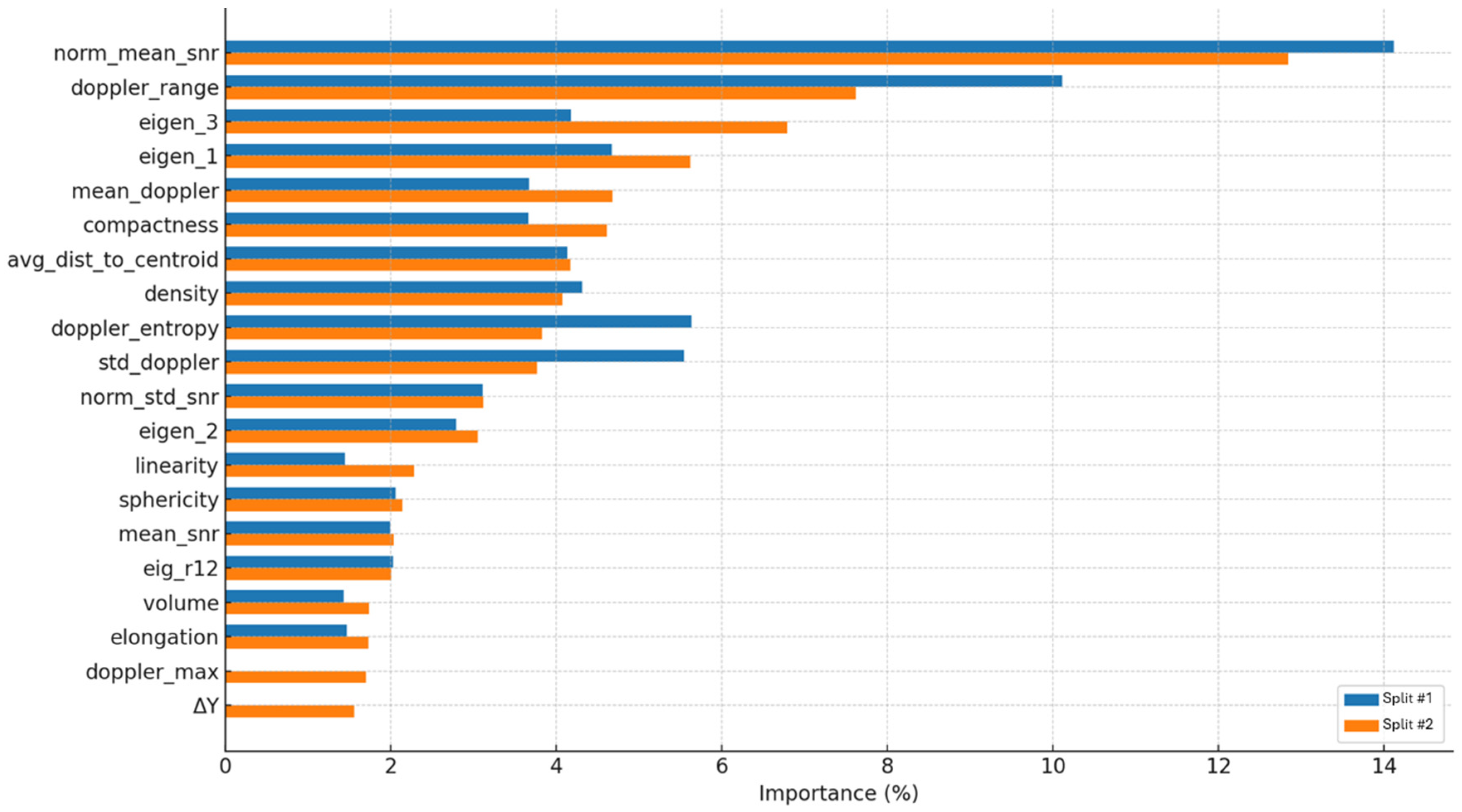
The feature importance analysis for the Random Forest model is illustrated via Figure 11 below. Evidently, the “norm_mean_snr” and “doppler_range” are by far the most influential features across both Split #1 and Split #2, contributing significantly to the model’s ability to discriminate between “Dock” and “No Dock” clusters. These features reflect the average intensity and velocity spread of the radar returns, which are strongly correlated with the presence of nearby reflective structures like docks. Geometric descriptors such as “eigen_3”, “eigen_1”, and compactness also rank highly, indicating that the shape and distribution of radar points within a cluster carry essential spatial information for classification. While most feature contributions remain consistent across sets, some variations—such as the increased importance of ΔY and “doppler_max” in Split #2—suggest that the model slightly shifts its focus depending on the environmental characteristics of each port configuration, reinforcing its adaptability to varying radar scenes.

Overall, Random Forest emerges as a robust and interpretable baseline. Its strength lies in its high precision on critical “Dock” detections, making it suitable for systems where minimizing false alarms is essential. The model’s ability to adapt across different port configurations, though slightly limited in recall under domain shifts, highlights the balance between simplicity and effective performance.

6.4. XGBoost-Based Classification and Resutls

6.4.1. XGBoost Model Architecture

XGBoost, a gradient-boosted decision tree method, was applied using the same engineered features as in the Random Forest model. Its ability to sequentially correct classification errors from prior trees, along with regularization mechanisms, makes it particularly suitable for structured data with class imbalance. To optimize performance, the model was tuned via randomized search across a range of hyperparameters, with the final configuration including 300 estimators, a learning rate of 0.05, and scale_pos_weight ≈ 1.76 to compensate for the underrepresented “Dock” class.

6.4.2. XGBoost Model Results

On the Split #1 test set, XGBoost achieved excellent performance, with precision and recall balanced across both classes. For the “Dock” class, the model attained a precision of 95.8%, a recall of 92.2%, and an F1-score of 94.0%, reflecting its ability to both detect most dock-related clusters and maintain low false positive rates. Similarly, the “No Dock” class reached a recall of 97.6% and an F1-score of 96.5%, showing strong generalization to negative examples as well.

When tested on Split #2, which contains a different combination of ports to simulate domain shift, XGBoost preserved nearly identical performance. The “Dock” class again achieved precision of 95.8% and recall of 92.2%, identical to Split #1, while the “No Dock” class reached precision of 95.5%, recall of 97.6%, and an F1-score of 96.5%.

These results are summarized in the following

Table 7. Results of XGBoost models for Split #1 and Split #2.

	Split #1		Split #2
	Dock	No-Dock	Dock	No-Dock
Precision (%)	95.8	95.5	94.5	93.7
Recall (%)	92.2	97.6	88.1	97.2
F1-score (%)	94.0	96.5	91.2	95.4

:

Overall, XGBoost demonstrates a high generalization ability and stable performance across datasets, maintaining balanced precision and recall. While slightly more cautious in predicting “Dock” clusters in Split #2, it effectively avoided false positives and sustained excellent accuracy for “No Dock” predictions. This makes XGBoost a strong candidate with practical applicability in operational radar-based classification systems.

6.4.3. XGBoost Feature Importance

The feature importance analysis for the XGBoost model highlights an emphasis on fewer but more influential features compared to Random Forest. As seen in the bar chart in Figure 12, “doppler_range” emerges as the single most influential factor across both Split #1 and Split #2, capturing the spread of radial velocities within a cluster.

The second most important feature is “norm_mean_snr”, which consistently ranks high across both splits. This measure of normalized reflection strength indicates that dock surfaces have distinctive SNR returns, in contrast to the various other detected clusters. Eigenvalue-based geometric descriptors, particularly “eigen_1” and “eig_r12”, also contribute meaningfully, emphasizing the role of structural shape in complementing Doppler and intensity cues.

Compared to Random Forest, XGBoost assigns less weight to secondary geometric or temporal features, focusing instead on a few highly discriminative variables. This behavior underscores the model’s gradient-boosting nature, which tends to exploit dominant patterns more aggressively. Despite this concentration, both splits demonstrate consistent rankings, suggesting that the learned feature hierarchy is robust to different environmental configurations.

6.5. PointNet-Based Classification and Results

PointNet, a deep learning architecture specifically designed for processing raw point clouds, directly processes the radar point clouds without the need of feature extraction [17]. This model’s ability to handle raw data efficiently makes it highly suitable for real-time applications, where preprocessing time is critical. Each point is passed through a shared multilayer perceptron (MLP), followed by a global max-pooling layer that extracts the most salient features, ensuring invariance to input ordering and varying point cloud sizes.

In this work, the PointNet architecture was implemented and trained from scratch; no transfer learning or pre-trained weights were used. All layers of the network—including three 1D convolutional layers with batch normalization and ReLU activation, a global max-pooling layer, two fully connected layers with dropout and batch normalization, and a final fully connected classification layer—were trained jointly. Training was performed in PyTorch (Stable 2.8) using the Adam optimizer with class-weighted cross-entropy loss to address class imbalance. Early stopping based on validation F1-score was applied to avoid overfitting, and the best model checkpoint was later evaluated on the test set.

On the Split #1 test set, PointNet achieved strong and balanced classification results. The model obtained an F1-score of 96.4% for the “Dock” class and 97.8% for the “No Dock” class. Precision values reached 95.5% and 98.4%, respectively, while recall remained equally high at 97.3% for both classes. Moving on to Split #2, which represents a different combination of ports and radar conditions, PointNet continued to perform reliably. It achieved 97.0% F1-score for “Dock” and 98.2% for “No Dock.” Precision remained high for both classes, at 95.3% (Dock) and 99.2% (No Dock), while recall reached 98.7% and 97.1%, respectively. These results suggest that PointNet effectively generalizes across environments, preserving its ability to identify dock-like structures and discriminate them from open water or noise.

These results are summarized in the following

Table 8. Results of PointNet model for Split #1 and Split #2.

	Split #1		Split #2
	Dock	No-Dock	Dock	No-Dock
Precision (%)	95.5	98.4	95.3	99.2
Recall (%)	97.3	97.3	98.7	97.1
F1-score (%)	96.4	97.8	97.0	98.2

:

6.6. Graph Neural Networks (GNN)-Based Classification and Results

Graph Neural Networks [26] are employed to directly model the spatial structure of radar point cloud clusters by treating each detection as a node and encoding local geometric relationships through k-nearest neighbor graphs. Herein, each node’s input features include normalized (x, y, z) coordinates, Doppler velocity, and SNR. The network then propagates information across the graph using two graph convolution layers, followed by ReLU activations, dropout, and a global mean-pooling layer that aggregates node embeddings into a compact graph representation for classification

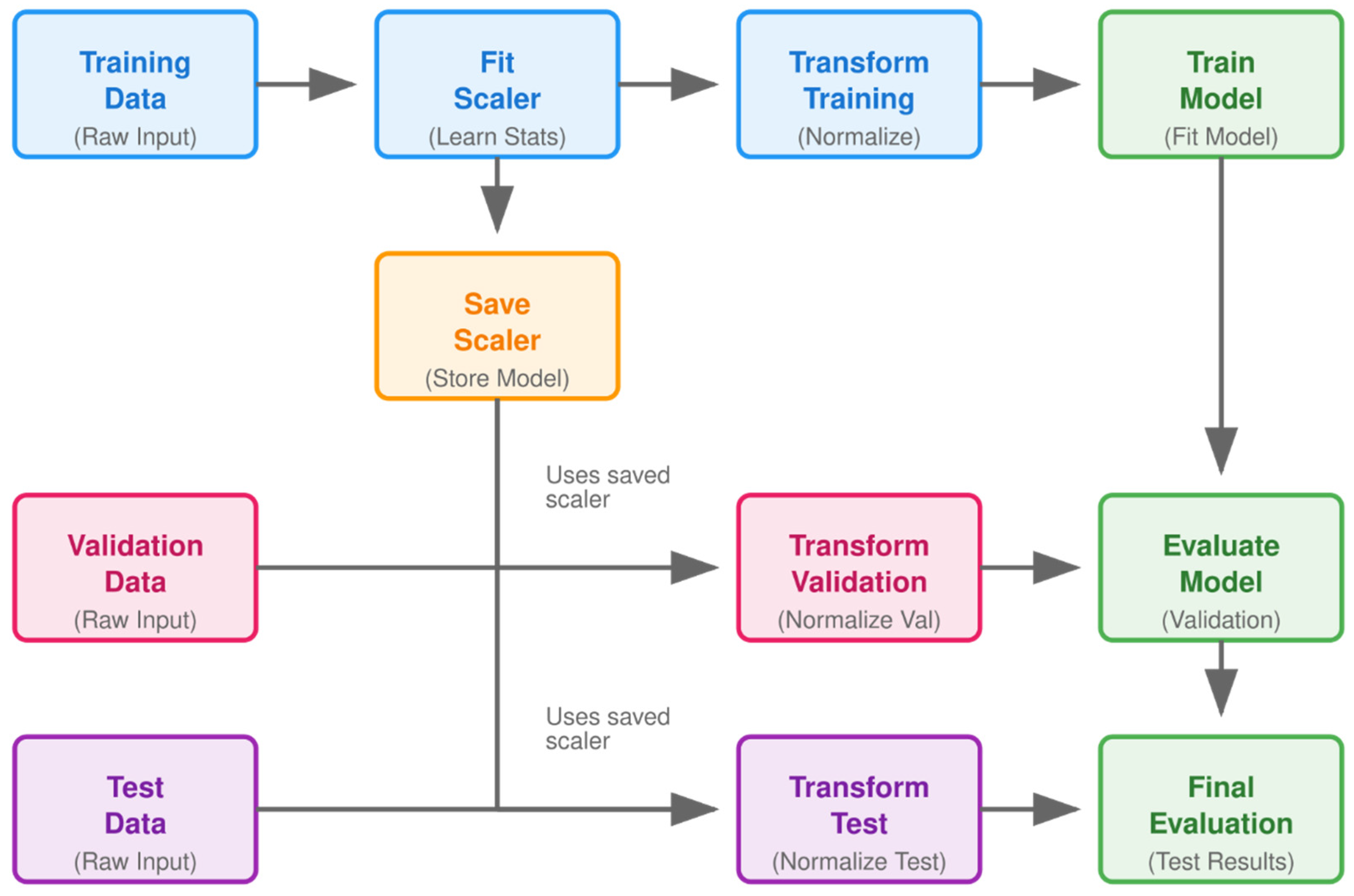
Unlike traditional models that rely on handcrafted features, the GNN operated directly on the raw point structure, making it well suited for complex, irregular input. The model was implemented and trained from scratch in PyTorch Geometric, without the use of pretrained weights or transfer learning. All preprocessing followed a consistent pipeline, where the scaler was fit exclusively on the training data and then reused for validation and test sets, ensuring no information leakage across splits. The overall workflow is illustrated in Figure 13 which shows how the raw radar point clouds were normalized, the model trained and subsequently evaluated on validation and test sets.

Regarding the performance results of our proposed GNN, it achieved strong performance in both splits. On the Split #1 test set, the GNN achieved a recall of 98.8% and precision of 95.3% for the “Dock” class, resulting in only 21 false negatives out of 1711 dock clusters. The “No Dock” class also showed robust results, with 97.1% recall and 99.3% precision. On the Split #2 test set, the GNN again delivered high accuracy, reaching a recall of 92.0% and precision of 93.2% for the “Dock” class, while the “No Dock” class achieved 96.3% recall and 95.7% precision.

These results are summarized in the following

Table 9. Results of GNN model for Split #1 and Split #2.

	Split #1		Split #2
	Dock	No-Dock	Dock	No-Dock
Precision (%)	95.3	99.3	93.2	95.7
Recall (%)	98.8	97.1	92.0	96.3
F1-score (%)	97.0	98.2	92.6	96.0

:

6.7. Model Comparison

6.7.1. Model Results

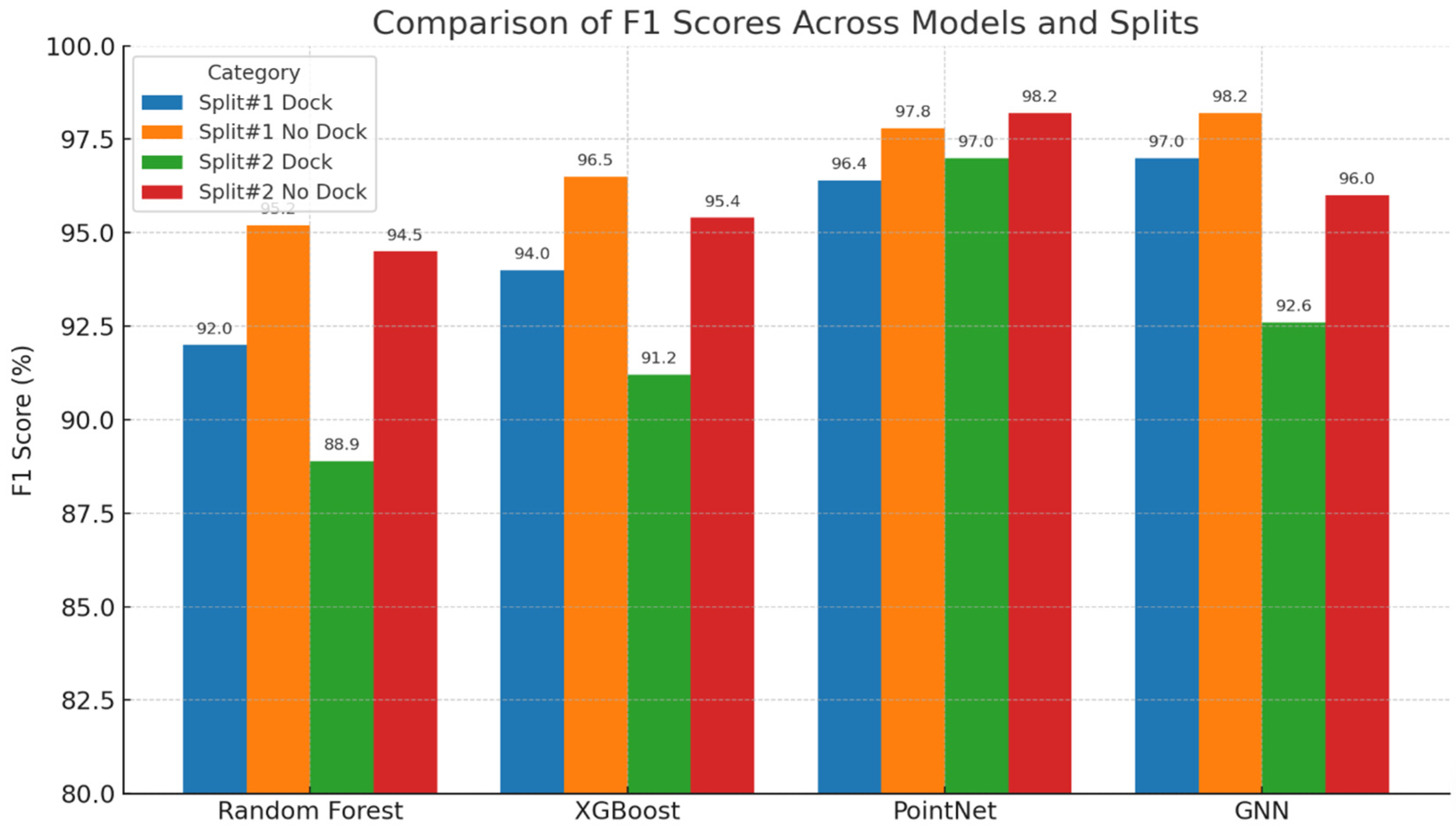
To provide a clear overview of the classification results, the F1-scores of all evaluated models (Random Forest, XGBoost, PointNet, and Graph Neural Networks) are summarized and compared in Figure 14. The distribution highlights that PointNet achieved the best overall performance, reaching up to 98.2% for the No-Dock class and 97.0% for the Dock class, while GNNs followed closely with slightly lower stability across dataset splits. In contrast, the feature-based models (Random Forest and XGBoost) achieved lower F1-scores, particularly in the Dock class of Split #2, indicating less robust generalization when tested on unseen ports. This comparison underscores the advantage of deep learning models that can directly interpret raw radar point cloud data over feature-based approaches.

6.7.2. Inference Time

While the dataset constitutes the primary contribution of this work, for scaling purposes and as a rough estimate we hereby provide the total delay time from first target detection to classification output. This delay was measured on a standard PC equipped with an Intel i7-4790K processor and an NVIDIA GTX 750 GPU. The preprocessing step, from raw radar signals to filtered clusters, requires approximately 1.27 ms. The subsequent classification delay varies with the model employed: Random Forest ≈ 2.61 ms, XGBoost ≈ 2.68 ms, PointNet ≈ 4 ms, and GNN ≈ 14 ms. Considering that the anticipated ship velocity during berthing does not exceed 1 m/s, these delays are regarded as fit for real-time berthing operations. Overall, the results indicate that all tested methods are fast enough for practical deployment, with only the GNN showing comparatively higher but still acceptable latency. Furthermore, even though the aforementioned time delay measures are measured on a standard PC, not much deviation is expected upon implementation on board powerful embedded computing units (contemporary Raspberry or NVIDIA Nano units, or similar equipment).

7. Conclusions

This paper presents development of a comprehensive dataset, namely Radar-based Berthing-Aid Dataset (R-BAD), that emerged due to the evolution of a radar-based berthing aid system, its deployment onboard a fully operational Ro-Ro/Passenger ferry ship, and its subsequent testing across a two-month period in real-life conditions. The proposed R-BAD dataset includes radar and camera sensor data that are synchronized, timestamped and geo-stamped. The R-BAD dataset covers all phases of berthing, including arrivals, departures, cruising, and port idle maneuvers. Encompassing approximately 69 h of radar data, it represents a unique resource explicitly designed for developing, validating, and benchmarking advanced machine learning models for short-range maritime obstacle detection. Furthermore, the applicability of the proposed dataset was tested vs. classification performance of four different classifier types (Random Forest, XGBoost, PointNet, and Graph Neural Networks). Notably, PointNet exhibited the best overall performance, achieving the highest F1 scores and consistent generalizability across unseen ports. Its ability to directly process raw radar point clouds highlights its suitability for real-time operational scenarios.

As a concluding remark, the developed radar-based platform illustrates that affordable FMCW radars, combined with modern machine learning methods, can form the basis of a cost-efficient berthing assistance system. Such systems have the potential to increase safety, reduce human error during docking, and provide valuable decision-support tools for vessel operators and port authorities. Another point of interest is that, due to safety concerns, the radar was deployed at a position on the ship that is sub-optimal. The high rise from the sea level and the high angle of detection are competing with radar range and field-of-view exploitation. Despite this fact, the performance of all clustering, tracking and classification methods is very satisfactory, thus demonstrating a promising pathway for future implementations—either retrofits or system installments at newly built ships.

Finally, the proposed R-BAD dataset and the developed codes are openly accessible on Zenodo [12] and GitHub [27], respectively, and thereby made available to everyone for research and further development in the field of maritime operations.