Abstract
Offline reinforcement learning suffers from critical vulnerability to data corruption from sensor noise or adversarial attacks. Recent research has achieved a lot by downweighting corrupted samples and fixing the corrupted data, while data corruption induces feature entanglement that undermines policy robustness. Existing methods fail to identify causal features behind performance degradation caused by corruption. To analyze causal relationships in corrupted data, we propose a method, Robust Causal Feature Disentanglement(RCFD). Our method introduces a learnable causal feature disentanglement mechanism specifically designed for reinforcement learning scenarios, integrating the CausalVAE framework to disentangle causal features governing environmental dynamics from corruption-sensitive non-causal features. Theoretically, this disentanglement confers a robustness advantage under data corruption conditions. Concurrently, causality-preserving perturbation training injects Gaussian noise solely into non-causal features to generate counterfactual samples and is enhanced by dual-path feature alignment and contrastive learning for representation invariance. A dynamic graph diagnostic module further employs graph convolutional attention networks to model spatiotemporal relationships and identify corrupted edges through structural consistency analysis, enabling precise data repair. The results exhibit highly robust performance across D4rl benchmarks under diverse data corruption conditions. This confirms that causal feature invariance helps bridge distributional gaps, promoting reliable deployment in complex real-world settings.
1. Introduction
Offline reinforcement learning (RL) addresses the critical challenge of learning optimal policies solely from pre-collected, static datasets without real-time environment interaction [1]. This paradigm is essential for applications where online exploration is impractical, costly, or unsafe. However, conventional offline RL methods exhibit significant vulnerability to data corruption, which arises from sensor noise, adversarial tampering, or environmental perturbations [2]. Such corruption manifests as random noise or adversarial perturbations that optimize systematic disruption and undermine both policy robustness and generalization [3,4,5,6,7].
These vulnerabilities are particularly concerning in high-stakes domains where policy failures can have severe consequences. In autonomous robotics, adversarial attacks on perception systems could result in catastrophic navigation failures in safety-critical environments such as surgical robots or autonomous vehicles [8,9]. Financial trading systems face comparable risks, where market data corruption or adversarial manipulation could trigger substantial economic losses and systemic market instability [10,11]. The importance of corruption-robust methods extends equally to robust control and safety fault-tolerant control systems [12,13,14,15].
The criticality of these applications demands robust offline RL methods that can maintain reliable performance despite data corruption. This motivates the development of causally robust approaches that can identify and mitigate corruption-induced feature entanglement while preserving the causal relationships essential for safe and reliable decision-making.
Recent research has achieved a lot. RIQL [5] leverages Huber loss and quantile estimators to handle heavy-tailed target distributions caused by dynamics corruption, while RDT [7] integrates embedding dropout and iterative data correction to mitigate corrupted inputs in sequential modeling. TRACER [6] model corruption-induced uncertainty via variational inference, using entropy-based weighting to downweight corrupted data. While RDT employs embedding dropout to improve robustness against erroneous inputs, it operates without understanding underlying causal relationships between state variables. The method’s iterative data correction process can identify corrupted actions and rewards but lacks theoretical grounding to distinguish corruption-sensitive features from those essential for environmental dynamics.
RIQL’s fundamental limitation stems from its reliance on temporal difference learning with Huber loss mechanisms that, while effective against dynamics corruption, cannot address feature entanglement at the representation level. TRACER’s uncertainty quantification gaps manifest in its entropy-based weighting mechanism, which downweights corrupted samples based on aggregate uncertainty without understanding specific causal mechanisms underlying corruption effects.
Existing approaches primarily focus on mitigating the performance degradation caused by damaged data, failing to explore the underlying causal relationships behind data corruption. To address these fundamental limitations, this work introduces the first causal-theoretic approach to data corruption offline reinforcement learning that explicitly models and exploits the distinction between causal features governing environmental dynamics and corruption-sensitive non-causal features. Our approach recognizes that data corruption induces systematic feature entanglement that can be formally addressed through structured causal modeling and targeted interventions.
This paper proposes a robust offline reinforcement learning framework based on causal feature invariance: Robust Causal Feature Disentanglement (RCFD). Its core innovations are as follows:
- Learnable Feature Disentanglement Mechanism: Integrating the CausalVAE framework to disentangle the corrupted data into causal and non-causal features (vulnerable to interference) provides formal guarantees of identifiability through structured causal models under idealized assumptions. Theoretically, this disentanglement confers a robustness advantage under data corruption conditions;
- Causal-Preserving Perturbation Training: This is conducted by generating samples and applying gaussian perturbations to non-causal features via counterfactual interventions while designing dual-path feature alignment loss and contrastive loss to enforce perturbation-invariant causal representations;
- Dynamic Graph Diagnosis and Reconstruction: This is conducted by employing graph convolutional attention networks to model spatiotemporal causal relationships among state variables, identifying corruption-sensitive edges through graph structure consistency loss to enable precise corrupted-data repair and smooth dynamic recovery.
Our experimental results demonstrate that the RCFD method broadly outperforms other baselines under data corruption conditions. This validates that the causality-based disentanglement approach effectively discerns the underlying causal relationships behind data corruption scenarios, thereby leveraging this insight to mitigate the impact of corrupted data.
2. Related Works
2.1. Offline Reinforcement Learning
Offline reinforcement learning addresses the critical challenge of learning policies from static datasets without environment interaction. Early approaches primarily tackled distributional shifts through policy constraints or value regularization. Methods like BCQ [16] and BEAR [17] enforced explicit policy constraints via action-space restrictions or MMD divergence, while BRAC [18] introduces behavioral constraints into actor–critic frameworks. These methods often induced excessive conservatism, limiting policy improvement potential. Concurrently, value regularization methods emerged to counter overestimation of out-of-distribution (OOD) [19,20,21,22] actions. CQL [23] learned conservative Q-functions by penalizing OOD actions, while IQL [24] approximated optimal in-distribution actions by estimating state-conditional upper expectiles of Q-values. Recent advances emphasize sequence modeling and diffusion policies. The Q-Transformer [25] integrated Transformer-based trajectory modeling with Q-learning, using Q-value regularization to bias action selection toward high-return behaviors. These innovations collectively address core challenges—distribution shifts, OOD actions, and trajectory stitching—while balancing policy improvement with safety constraints. FISOR [26] enforces hard safety constraints via the HJ reachability theory. ORL-RC [27] blends policy constraints and value regularization to mitigate over-pessimism. It uses hybrid policy evaluation with behavior cloning to balance conservatism and optimality.
2.2. Data Corruption Reinforcement Learning
Offline RL faces significant challenges when training data containing corrupted transitions due to sensor errors or adversarial tampering. RIQL [5] solves the problem of heavy-tail targets of Q functions under dynamics corruption conditions via Huber loss and quantile estimation; then they propose TRACER [6], leveraging Bayesian inference to model action-value uncertainty and downweight corrupted samples through entropy-weighted learning. Ye et al. [28] achieves additive dependence on corruption under general function approximation by controlling weighted uncertainty sums via the eluder dimension and new analytical techniques. Mandal et al. [29] model corruption in RLHF via state-confounded MDPs. Under conditions of low sample efficiency, Xu et al. [7] employed the sequence modeling method and the Decision Transformer [30] (DT) to leverage contextual knowledge, thereby enhancing data utility and mitigating the impact of data corruption.
2.3. Disentangled Reinforcement Learning
Disentangled reinforcement learning approaches focus on learning representations that explicitly separate entangled features to enhance robustness and generalization, with several recent methods leveraging auxiliary tasks for disentanglement in diverse RL settings. For example, SEAR [31] uses agent masks as weak supervision to impose an auxiliary reconstruction loss, forcing the policy to disentangle robot-centric features from environmental factors via variational inference, which significantly improves sample efficiency in visual control tasks by reducing spurious correlations across simulated robotics environments. Complementing these, CMID [32] formulates disentanglement as an adversarial RL task by minimizing conditional mutual information between features given a conditioning set derived from Markov decision process dynamics, enabling resilience to correlation shifts.
3. Preliminarys
3.1. Offline Reinforcement Learning
Reinforcement learning (RL) fundamentally addresses the challenge of how an autonomous agent should learn to make optimal sequential decisions through interactions within an environment. The standard setup is formalized as a Markov decision process (MDP). An MDP is mathematically represented by a tuple as follows:
where S denotes the set of possible states an agent can perceive; A represents the set of actions available to the agent, defines the state transition probability distribution dictating the likelihood of transitioning to state s’ after taking action a in state s; signifies the immediate reward function specifying the scalar reward obtained after transitioning from s to via action a; and in (0, 1] is the discount factor, determining the present value of future rewards and balancing immediate versus long-term gain.
Offline reinforcement learning tackles the problem of learning effective policies () solely from a pre-collected, static dataset of interaction trajectories, where
The dataset is generated by a behavioral policy, , without any further online interaction with the actual MDP during training. This constraint introduces the critical challenge of distribution shifts, necessitating specialized approaches for policy evaluation and optimization under the offline data regime.
3.2. Causal Inference
In reinforcement learning, environmental states encountered by agents contain both causal features that directly influence decision-making and non-causal features susceptible to noise disturbances. Causal inference formally establishes its separability through interventional invariance and counterfactual invariance. Specifically, when the environment satisfies the causal sufficiency assumption (all common causes are observable) and structural stability assumption (causal relationships remain time-invariant), state features can be uniquely identified and separated.
Interventional invariance serves as the cornerstone: For any intervention (forcing non-causal feature to value ), the causal feature preserves the distribution of rewards and state transitions:
where denotes the intervention scope, proving that the non-causal features do not alter decision dynamics.
3.3. Data Corruption
Data corruption manifests in two primary forms that require distinct mathematical characterization. Random corruption models naturally occurring noise inherent in physical systems, such as sensor inaccuracies or environmental interference. This phenomenon is formally described through additive perturbation:
where the stochastic term sampled from a uniform distribution introduces isotropic deviations scaled by the dataset’s global standard deviation () and governs corruption intensity, with higher values simulating severe measurement degradation.
Conversely, adversarial corruption represents intentional manipulation designed to maximize systemic disruption. It is modeled as a constrained optimization problem as follows:
This minimizes a pretrained agent’s Q-value (). The generated corruptions systematically exploit decision boundaries, simulating sophisticated attacks.
4. Methods
This section presents a robust framework for handling data corruption in RL. The approach formalizes the separation of causality-corrupted features, designs targeted perturbation mechanisms, implements spatiotemporal fault diagnosis, and integrates multi-objective optimization. Figure 1 illustrates the overall architecture.
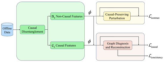
Figure 1.
Architecture of RCFD.
State observations () first pass through the CausalVAE encoder to obtain ; then the perturbation module operates on to generate counterfactual samples (), while the GCAN module processes temporal sequences to detect corrupted edges and provide structural feedback for repair. All modules are unified through a multi-objective loss function that balances feature invariance, perturbation robustness, and structural consistency.
4.1. Causal Feature Disentanglement
We fundamentally reimagine the feature disentanglement mechanism by integrating the CausalVAE [33] framework. Unlike existing causality-aware RL methods that focus on clean data scenarios, our approach specifically targets corruption-induced feature entanglement in offline datasets through causal structure modeling. The framework implements a structured causal model (SCM) [34,35] layer that transforms independent exogenous factors into causally structured endogenous representations. Unlike heuristic separation methods, this approach provides learning objectives through guarantees of identifiability under idealized conditions while enabling explicit counterfactual interventions. The architecture establishes a bijective mapping between state observations and disentangled causal/non-causal representations:
where captures non-causal noise patterns and represents invariant causal features governing environmental dynamics. The adjacency matrix A encodes directional dependencies between variables and satisfies Directed Acyclic Graph (DAG) constraints through the acyclicity regularization .
Building upon the original structural causal model (SCM) framework, we formalize the causal disentanglement process by introducing a variational inference framework. The generative process for the observed state is defined as follows:
where represents the causal features and represents the non-causal features.
We introduce a variational lower bound (ELBO) to help the optimization objective learn the encoder parameters (). The derivation of the variational lower bound is defined as follows (refer to Appendix A.1):
where denotes the encoder, while and represent the prior distributions. The KL divergence term is factorized as follows:
Maximizing the ELBO ensures that the variational posterior closely approximates the true, intractable posterior distribution over causal and non-causal features. Crucially, the structure of the KL divergence term (specifically, its factorization into separate terms for and as shown in Equation (9)) facilitates the disentanglement process. By minimizing this KL divergence between the variational posterior and the factorized prior , the model is encouraged to separate the latent space into distinct causal features () that govern dynamics and non-causal features () sensitive to corruption, thereby achieving the core goal of causal disentanglement.
We define the marginal distribution of causal features under corruption as follows:
Since corruption primarily affects non-causal features, the distributional shift in the causal space is significantly attenuated as follows:
where TV is total variation distance between probability distributions and represents the attenuation factor (typically ), reflecting how corruption in the complete state space translates to changes in causal features. Consequently, the performance loss of the causal disentanglement strategy is bounded by the following equation:
To quantify the robustness advantage of causal disentanglement, we define the robustness gain as follows:
Substituting the derived bounds yields the following equation:
Given that and , we obtain the following equation:
This theoretical result establishes that under the causal invariance assumption, for any corruption rate , there exists a constant such that
It is important to note that the theoretical bounds presented in this analysis serve primarily as qualitative analytical tools rather than quantities requiring precise numerical computation in practice. These expressions formalize the mechanistic relationship between causal disentanglement and robustness: corruption effects are attenuated when projected into the causal subspace (attenuation factor ), with performance degradation scaling proportionally to corruption intensity () and distributional shift magnitude. The KL divergence terms appearing in these bounds are analytical constructs that help understand the underlying mechanisms, not parameters requiring estimation during algorithm execution. In high-dimensional continuous state spaces without known parametric forms, these quantities cannot be reliably computed.
To empirically validate the effectiveness of our causal feature disentanglement mechanism, we visualize the learned feature representations using t-Distributed Stochastic Neighbor Embedding (t-SNE) analysis. Figure 2 demonstrates the clear separation achieved between causal and non-causal features through our RCFD framework.
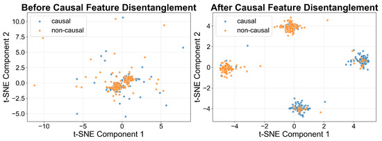
Figure 2.
T-SNE visualization of feature disentanglement.
As illustrated in Figure 2, the original state representations exhibit significant feature entanglement, where causal and non-causal components are intermixed and indistinguishable in the latent space. This entanglement makes the learned policy vulnerable to data corruption, as the model cannot differentiate between corruption-sensitive features and those essential for environmental dynamics. Our causal disentanglement mechanism demonstrates remarkable separation after application. The causal features (represented by blue clusters) form distinct, well-separated regions from the non-causal features (represented by red clusters).
This visualization provides compelling evidence that our causal disentanglement mechanism effectively addresses the fundamental challenge of feature entanglement in corrupted offline RL datasets. Moreover, we supplement these qualitative results with rigorous quantitative evaluation methods to ensure statistical validity of the observed separation. We quantify the degree of feature separation using mutual information between causal and non-causal feature representations. We employ kernel density estimation to approximate the probability distributions and compute mutual information as follows:
where is the joint probability density, while and are marginal densities estimated using Gaussian kernels with the bandwidth selected via cross-validation.
Our experimental results demonstrate that mutual information between causal and non-causal features significantly decreases to 0.23 after disentanglement under the RCFD framework. Our mutual information estimation employs kernel density estimation with Gaussian kernels to approximate probability densities. The estimation uses state pairs sampled from trained encoder outputs, with the bandwidth selected via cross-validation. To assess estimator reliability, we conduct bootstrap resampling with 500 iterations, yielding a 95% confidence interval of with a standard deviation of , indicating reasonably stable estimation across data subsamples.
The t-SNE visualization in Figure 2 provides qualitative corroboration, showing clear spatial separation between causal and non-causal feature clusters with minimal overlap regions. This visual evidence is consistent with quantitative MI measurements indicating successful but imperfect disentanglement.
The visualization and quantitative assessments provide compelling evidence that our causal disentanglement mechanism effectively addresses the fundamental challenge of feature entanglement in corrupted offline RL datasets. The clear separation enables our subsequent causality-preserving perturbation training to selectively intervene in non-causal features while preserving the integrity of causal dynamics, ultimately leading to more robust policy learning under data corruption scenarios.
4.2. Causality-Preserving Perturbation Mechanism
Based on the counterfactual reasoning framework [34,35,36,37], the perturbation mechanism operates specifically on the non-causal features extracted by the encoder. The module receives the factorized state representation and applies selective interventions to simulate corruption scenarios while maintaining causal consistency. This targeted approach leverages the clear separation achieved by the disentanglement module, ensuring that perturbations do not interfere with environmentally critical causal features (). Based on a disentangled feature space (), our conditional intervention generator is implemented as follows:
where is a Gaussian noise vector with . The state intervention probability p is set to 0.2, indicating that we intervene on 20% of states per batch by perturbing their non-causal features through additive Gaussian noise (). This design preserves the causal features to maintain environmental dynamics consistency while disturbing the non-causal features to simulate data corruption.
The counterfactual samples enhance feature invariance via a dual-path framework:
where is the causal feature extractor. Feature alignment minimizes the discrepancy in causal features between original states and perturbed states.
To further enhance the robustness of the model against data corruption, we introduce a contrastive learning loss function that enforces feature invariance between clean states and their perturbed counterparts. This loss function operates within the causal feature space, minimizing the discrepancy between the representations of original states () and counterfactual states () generated through our perturbation mechanism. The contrastive loss function is formally defined as follows:
where are positive pairs, is the perturbation of , is randomly sampled from the dataset constituting the negative sample set N, and is the temperature hyperparameter, where .
This design ensures that the model learns representations invariant to corruption-induced variations, which is critical for maintaining performance under adversarial or noisy conditions.
4.3. Dynamic Causal Graph Diagnosis and Reconstruction
We propose a spatiotemporal-aware fault diagnosis module whose core innovation lies in modeling data corruption as a disruption of graph-structured causality among state variables. The graph convolution attention hybrid network (GCAN) module employs a principled approach to identify and reconstruct corrupted edges through structural consistency analysis.
In offline RL scenarios, we typically have limited prior knowledge about the causal structure among state variables. Our GCAN module addresses this challenge through a hybrid initialization strategy that combines minimal domain knowledge with data-driven structure learning. The core intuition is that corrupted data will exhibit abnormal attention patterns and violate the learned causal structure, enabling targeted detection and repair. First we start prior-based initialization. We utilize only basic structural assumptions available in most RL environments. For example, in locomotion tasks, we only assume that sequential state components may have dependencies, and the position and velocity of the same joint are related. Then given the limited prior knowledge, the GCAN primarily relies on data-driven learning to discover the causal graph structure. To handle the uncertainty from limited priors, we employ probabilistic initialization as follows:
where and are set based on the confidence level of available prior knowledge. For most connections where we have no prior knowledge, we use = = 1.
Given the sparse initial structure , we learn the complete causal graph through gradient-based optimization. We first embed the temporal state–action–reward sequences into node features:
where , , and represent the state, action, and reward at timestep t, respectively.
The adjacency matrix is then refined through attention-based learning that respects the initial structure, where
The complete structure learning objective combines reconstruction accuracy with structural constraints as follows:
where enforces DAG constraints and regularizes deviation from prior knowledge.
Once the causal structure is learned, we leverage attention weights as corruption indicators. For each timestep t, we compute the attention-based edge importance scores as follows:
where H is the number of attention heads. Corrupted edges are identified through temporal consistency analysis.
For detected corrupted edges , we apply targeted interventions as follows:
where represents learned repair weights and comes from the structural prediction using uncorrupted edges.
4.4. Multi-Objective Optimization
The RCFD framework integrates the diverse loss functions derived from causal feature disentanglement, perturbation training, and graph-based diagnostics into a unified multi-objective optimization objective, and it is formulated as follows:
where serves as the behavioral cloning loss, which anchors the policy to the offline dataset by minimizing action distribution discrepancies, ensuring stable learning under distributional shifts.
This comprehensive objective function aims to harmonize the competing goals of policy fidelity, causal invariance, noise robustness, and structural integrity.
5. Experiment
In this section, we test our method in the D4rl dataset [38]. We set the dataset to be under different data corruption conditions, including both random and adversarial attacks on states, actions, and rewards.
5.1. Environment Setting
The evaluation environment of our method is set on D4RL, which stands as the most widely adopted offline reinforcement learning dataset and is extensively utilized under data-deficient conditions. Three core tasks were selected, HalfCheetah, Walker2d, and Hopper, each representing distinct locomotion challenges. For each task, datasets such as “Halfcheetah-medium-replay-v2” were employed, characterized by approximately 100,000–200,000 samples, as detailed in Appendix B.3. Our experiments are organized into three tasks and three diverse data corruption conditions, and both random and adversarial corruption are included. The corruption rate is set to 0.3, and the corruption scale is 1 for the main results. Random corruption involved additive Gaussian noise scaled by the dataset’s global standard deviation, while adversarial corruption is introduced through the Projected Gradient Descent attack with a pretrained EDAC [39] agent.
Following the established protocols from RIQL [5] and other robust offline RL works, we ensure a fair comparison by carefully aligning all experimental parameters and hyperparameter settings with the baseline methods. Our implementation adopts identical network architectures, learning rates (), batch sizes (256), and training procedures (1M environment steps) across all compared methods to ensure that performance differences can be attributed to algorithmic improvements rather than implementation variations.
We combine our method with the baselines of offline reinforcement learning methods under data corruption conditions, such as IQL [24], CQL [23], RIQL [5], RDT [7], and the causal RL baseline CausalExploration [40]. All experiments are trained for 1m environment steps using four random seeds.
5.2. Evaluation Under Random Corruption
We first test the performance RCFD under random corruption conditions. RCFD demonstrated resilience against random corruption, achieving a mean normalized score of 58.6 across all tasks and attack elements, as summarized in Table 1. This performance exceeded the nearest baseline RDT by approximately 16.27%, highlighting RCFD’s ability to mitigate feature entanglement through causal invariance.

Table 1.
Average normalized performance under random data corruption.
A pronounced performance advantage manifests in observation corruption scenarios for HalfCheetah and Hopper environments. In HalfCheetah, RCFD attains a score of 29.4, representing a 36.2% improvement over the second-best baseline RIQL (21.58). In Hopper, RCFD achieves a score of 84.27, substantially exceeding RDT’s performance of 65.6 by 28.5%, while simultaneously demonstrating perfect stability. These empirical findings substantiate the theoretical foundation that our causal disentanglement mechanism effectively isolates corruption-sensitive non-causal features from invariant causal dynamics, particularly when corruption primarily manifests as observational noise in specific locomotion paradigms.
Conversely, the Walker2d environment under observation corruption exposes a notable limitation in our approach. RCFD achieves a score of 44.65, underperforming relative to RDT (53.05) by 15.8%, despite outperforming RIQL (33.71). The performance disparity in Walker under observation corruption warrants detailed discussion. Walker’s bipedal locomotion involves complex interdependencies between sequential joint pairs where causal relationships are highly entangled. Unlike HalfCheetah’s relatively independent joint actuations or Hopper’s simpler single-leg dynamics, Walker requires coordinated balance control where observation corruption in one joint can cascade through the kinematic chain. Our current causal disentanglement mechanism, which assumes relatively sparse causal structures, struggles to capture these dense interaction patterns. The observed performance gap indicates the necessity for incorporating environment-specific structural priors into the causal feature learning process to accommodate the diverse causal architectures inherent in different robotic morphologies and control paradigms.
The results validate that causal feature disentanglement bridges distributional gaps, as corrupted samples were downweighted while invariant features maintained environmental dynamics.
5.3. Evaluation Under Adversarial Corruption
To further evaluate RCFD, we introduce adversarial data corruption under diverse data corruption scenarios. Under adversarial corruption, RCFD maintained robust performance with a mean score of 54.6, outperforming all baselines by approximately 15.92% over the the best-performing baseline (RIQL), as evidenced in Table 2. The causal disentanglement mechanism effectively reduces the distributional shift between clean and corrupted data.
Table 2.
Average normalized performance under adversarial data corruption conditions.
RCFD’s robustness depends strongly on the interplay between the morphology and dynamics of the environment and the specific corruption type. In Hopper and Walker2d, the method excels when adversarial corruption targets actions or rewards, as the GCAN-based repair and contrastive representation learning effectively mitigate the impact of such perturbations. However, in HalfCheetah and Hopper, sophisticated adversarial manipulation of state variables continues to expose weaknesses in the learned disentanglement. The causal invariance framework relies on causal sufficiency and structural stability assumptions that may be violated in real-world scenarios. Considering unobserved confounders that violate causal sufficiency, suppose an unobserved confounder U affects both observed state variable and reward r. The true causal model includes and , but our framework only observes . This violation affects RCFD because the encoder may incorrectly attribute variations caused by U to either or . If U is correlated with corruption patterns, the learned disentanglement becomes unreliable. Overall, the adversarial corruption evaluation confirms the efficacy of RCFD’s causal-feature-centric design in preserving policy integrity against structured, high-impact adversarial attack.
5.4. Ablation Experiments
5.4.1. Ablation Study on Different Modules
To analyze component contributions, we conduct ablation studies by sequentially removing core architectural elements. Ablation experiments were conducted to dissect RCFD’s core innovations, sequentially removing components to quantify their impact on corruption robustness, as shown in Figure 3. When the causal disentanglement mechanism was disabled, mean performance under random corruption dropped by 28.24%, emphasizing that feature separation is indispensable for mitigating entanglement. Similarly, omitting the causality-preserving perturbation training generates counterfactual samples via Gaussian noise in non-causal features. This reduced scores by 14.67% due to degraded invariance in causal representations. When the modification detection work of the GCAN’s damage data was ignored, the score dropped by 13.5%.
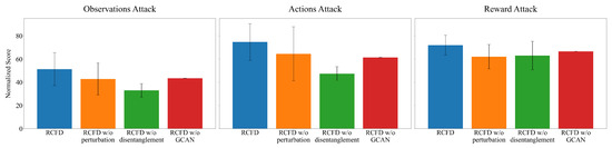
Figure 3.
Ablation experiments of RCFD in Hopper.
5.4.2. Ablation Study on Corruption Rates
To comprehensively evaluate RCFD’s robustness across varying corruption intensities, we conduct ablation studies on corruption rates ranging from 0.1 to 0.5 in the Walker environment. As the Figure 4 shows, This analysis examines how different corruption intensities affect the relative performance advantages of our method compared to baseline approaches.
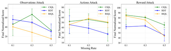
Figure 4.
Ablation experiments of corruption rates in Walker.
RCFD maintains consistently strong performance under reward corruption across all tested corruption rates. This consistent performance advantage validates our theoretical framework’s effectiveness in isolating reward-related corruption from causal dynamics. At the highest tested corruption rate, RCFD maintains functional performance across all corruption types.
These results validate our theoretical framework’s core premise: by explicitly modeling and preserving causal relationships, RCFD achieves superior robustness that scales effectively with corruption intensity.
5.4.3. Ablation Study on Hyperparameters
As the Figure 5 shows, the contrastive learning coefficient demonstrates a pronounced non-monotonic relationship with model performance across all corruption scenarios. At , the framework achieves optimal performance under corruption conditions. The dramatic performance drop at suggests that insufficient contrastive regularization fails to enforce adequate feature invariance between clean and perturbed states, allowing corruption-sensitive representations to dominate the learned policy. Conversely, excessive contrastive weighting at leads to over-regularization, constraining the model’s capacity to capture nuanced environmental dynamics and resulting in reduced performance scores.
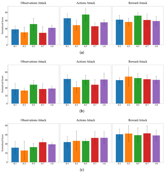
Figure 5.
The ablation experiment of the parameter in hopper. (a) Parameter . (b) Parameter . (c) Parameter .
The consistency regularization parameter exhibits a more stable performance profile, though with notable variations that illuminate the role of temporal structural coherence in corruption robustness. The optimal configuration occurs at . This configuration strikes an effective balance between structural constraint enforcement and model flexibility, enabling the dynamic graph diagnostic module to identify corrupted edges without imposing excessive rigidity on the learned causal relationships. Interestingly, the consistency parameter shows diminishing returns at higher values, with producing marginally reduced performance, suggesting that overly strict temporal consistency constraints can impede the model’s ability to adapt to legitimate environmental variations.
The causal regularization coefficient exhibits complex optimization dynamics that vary significantly across different corruption scenarios. Comprehensive analysis across all three attack vectors reveals that delivers the most robust overall performance.
6. Conclusions
This paper introduces Robust Causal Feature Disentanglement (RCFD), a novel framework for corruption-robust offline reinforcement learning. By integrating causal disentanglement, perturbation training, and dynamic graph diagnostics, RCFD fundamentally addresses feature entanglement induced by data corruption. The experiment results confirm that isolating causal invariance is effective for bridging distributional gaps in corrupted data. While RCFD demonstrates effectiveness on D4RL locomotion benchmarks, several limitations constrain broader applicability. Our framework relies on causal sufficiency and structural stability assumptions that may be violated in complex real-world scenarios. High-dimensional visual observations present challenges for causal structure learning in pixel space, requiring integration with world models or hierarchical representations to make causal discovery tractable. Partial observability fundamentally violates causal sufficiency since hidden states constitute unobserved confounders, necessitating extensions to belief-state representations and partial identification techniques. Future work will address these limitations through hierarchical causal models for vision tasks, online structure learning for non-stationary environments, and theoretical analysis under relaxed causal assumptions.
Author Contributions
Conceptualization, A.M.; methodology, A.M. and P.L.; software, A.M.; validation, X.S.; formal analysis, A.M. and X.S.; writing—original draft, A.M.; writing—review and editing, P.L.; supervision, P.L. All authors have read and agreed to the published version of the manuscript.
Funding
The authors gratefully acknowledge financial support from the National Natural Science Foundation of China (62376280).
Data Availability Statement
The original contributions presented in the study are included in the article, whilst further inquiries can be directed to the corresponding author.
Conflicts of Interest
On behalf of all authors, the corresponding author states that there are no conflicts of interest in any material discussed in this paper.
Abbreviations
The following abbreviations are used in this manuscript:
| RCFD | Robust Invariant Feature Disentanglement |
| RL | Reinforcement Learning |
| GCAN | Graph Convolution-Attention hybrid Network |
| DAG | Directed Acyclic Graph |
| OOD | Out of Distribution |
| DT | Decision Transformer |
| MDP | Markov Decision Process |
| SCM | Structured Causal Model |
Appendix A. Proof of Theorem
Appendix A.1. Variational Lower Bound (ELBO) Derivation
This appendix provides detailed derivations for key equations in Section 4.1. We prove Equation (8) (variational lower bound) and Equation (9) (KL divergence decomposition) based on the CausalVAE framework, assuming independence between causal features and non-causal features .
Proof of Equation (8).
Variational Lower Bound (ELBO)
The marginal likelihood of the observed state is as follows:
Introducing the variational posterior as an approximation to the true posterior , Jensen’s inequality gives the following:
Rewriting the right-hand side yields the following equation:
Adding and subtracting yields the following equation:
The term in parentheses is the KL divergence, where
Thus
Ignoring the constant term (as it does not affect optimization), we obtain Equation (8), where
□
Appendix A.2. Markovian Assumption
The Markovian assumption states that the future state depends only on the current state and action, not on the entire history of states and actions:
Under data corruption, this assumption extends to the disentangled feature space. We assume that causal features () maintain Markovian properties even under corruption conditions:
This assumption is critical because it ensures that our causal feature disentanglement preserves the fundamental decision-making structure of the MDP despite corruption in non-causal features.
Appendix A.3. KL Divergence Decomposition
The KL divergence is defined as follows:
Assuming the variational posterior factorizes as (conditional independence given ), where
Appendix A.4. Detailed Derivation of Theoretical Analysis for Causal Disentanglement Robustness
We first establish the foundational framework for theoretical analysis. Let the state distribution in the original environment be and the state distribution in the corrupted environment be . The state space can be decomposed into causal features c and non-causal features n, i.e., .
We make two key assumptions: (1) Causal invariance: causal features c play a decisive role in environmental dynamics, while non-causal features n are primarily affected by noise; (2) Corruption locality: data corruption primarily affects non-causal features, with limited impact on causal features.
Appendix A.4.1. Distributional Shift Analysis Under Corruption
In the corrupted environment, we define the marginal distribution of causal features as follows:
Since corruption primarily affects non-causal features, the distributional shift in the causal space is significantly attenuated:
where represents the attenuation factor (typically ) and is the corruption intensity, reflecting how corruption in the complete state space translates to changes in causal features.
To establish this bound, we consider the corruption process , where is the noise vector. Since corruption primarily affects non-causal features, we have . According to the definition of total variation distance,
Utilizing the properties of marginal distributions and corruption locality,
Appendix A.4.2. Bound Analysis of Policy Performance Loss
For a policy based on causal disentanglement, its performance loss under corruption is bounded by
Using the policy gradient theorem and performance difference decomposition,
where is the state visitation distribution of policy in the clean environment and is the advantage function in the corrupted environment.
Through Pinsker’s inequality and distributional shift bounds,
Appendix A.4.3. Quantitative Analysis of Robustness Gains
To quantify the robustness advantage of causal disentanglement, we define the robustness gain as follows:
where is a conventional policy and is a policy based on causal disentanglement.
The lower bound of the robustness gain is
For a conventional policy , its performance loss is bounded by the following equation:
Combining this with our previous result for causal disentanglement policies establishes the robustness gain bound.
Appendix A.4.4. Asymptotic Robustness Guarantee
Considering that and , we can further simplify the analysis. Under strong causal invariance conditions (), the robustness gain approaches
This theoretical result establishes that under the causal invariance assumption, for any corruption rate , there exists a constant such that
These theoretical results provide a rigorous mathematical foundation for the effectiveness of the RCFD method, demonstrating the theoretical advantages of causal feature disentanglement in improving the robustness of offline reinforcement learning.
Appendix A.5. Identifiability Constraints
The identifiability foundations in causal representation learning studies (e.g., CausalVAE) establish conditions under which causal factors can be theoretically recovered. These theoretical requirements include causal sufficiency where all common causes in the true causal graph must be observed, faithfulness where every d-separation in the causal graph must correspond to a conditional independence in the distribution, correct DAG specification where the constraint must align with the true acyclicity structure, and interventional diversity with sufficient coverage of interventional distributions to distinguish causal directions. In D4RL, practical limitations arise because no ground-truth causal graphs are available for validation, offline data is generated by behavioral policies without designed interventions, potential hidden confounders exist, our perturbation mechanism provides limited interventional diversity, and no verification protocol exists for the faithfulness assumption. What we achieve is a learned factorization that demonstrably improves corruption robustness. This leverages the theoretical identifiability foundations to design principled learning objectives (structural constraints, interventional perturbations, and invariance terms) that yield practically beneficial representations.
Appendix B. Environment Setting
Appendix B.1. Data Corruption Details
Following the corruption framework established in prior robust offline RL research, we implement comprehensive data corruption across all dataset elements to evaluate RCFD’s robustness under diverse attack scenarios.
- Random observation attack: We randomly sample a fraction c (corruption rate) of state transition tuples from the dataset and apply Gaussian noise perturbations to the selected states (), where , represents state dimensionality, denotes the dimensional standard deviation of all states in the dataset, and the corruption scale controls corruption intensity.
- Random action attack: Using the same sampling rate , we select state transition samples and apply perturbations to the actions , where , is the action dimensionality and represents the dimensional standard deviation of the action space.
- Random reward attack: For randomly selected samples, we replace original rewards with . The amplification factor is employed because offline reinforcement learning algorithms exhibit natural resistance to small-scale reward perturbations but experience performance collapse under large-scale corruption conditions.
In addition, adversarial data corruption is detailed as follows:
- Adversarial observation attack: We first pre-train an EDAC agent on clean data to obtain the Q-network and the policy . Subsequently, we implement gradient optimization attacks on a selected proportion of states, , where limits the maximum deviation for each state dimension. The optimization process employs Projected Gradient Descent with 100 iterations and a learning rate of 0.01 and clips the perturbation vector to the range after each update.
- Adversarial action attack: Utilizing the pre-trained agent, we implement similar attacks on the actions , where , with the optimization strategy consistent with state attacks.
- Adversarial reward attack: For reward signals, we adopt the following direct inversion strategy: . This method is based on the optimal solution properties of the minimization objective .
Appendix B.2. Tasks in D4RL
We classify a set of offline continuous control tasks from D4RL [38] datasets and provide a summary for each task in Table A1.
Table A1.
A detailed description of each task of the Gym-mujoco environment of the D4RL dataset in our experiment.
Table A1.
A detailed description of each task of the Gym-mujoco environment of the D4RL dataset in our experiment.
| Task | Allowed Steps | Samples |
|---|---|---|
| Halfcheetah-medium-replay-v2 | 101,000 | |
| Hopper-medium-replay-v2 | 200,920 | |
| Walker2d-medium-replay-v2 | 100,930 |
Appendix B.3. Hyperparameters
The full list of hyperparameters is presented in Table A2. Most of the environment configuration parameters remain consistent with those implemented in the official IQL [24] source code.


Figure A1.
The ablation experiment of some parameters in Hopper. (a) Parameter . (b) Parameter p. (c) Parameter .
Table A2.
A default set of hyperparameters used in our experiments.
Table A2.
A default set of hyperparameters used in our experiments.
| Parameter | Setting |
|---|---|
| Buffer size | 2 × 10⁶ |
| Batch size | 256 |
| Intervention prob | 0.2 |
| Intervention noise scale | 0.1 |
| 0.5 | |
| 0.5 | |
| 0.7 | |
| corruption range | 1.0 |
| corruption rate | 0.3 |
References
- Prudencio, R.F.; Maximo, M.R.; Colombini, E.L. A survey on offline reinforcement learning: Taxonomy, review, and open problems. IEEE Trans. Neural Netw. Learn. Syst. 2023, 35, 10237–10257. [Google Scholar] [CrossRef] [PubMed]
- Zhang, X.; Chen, Y.; Zhu, X.; Sun, W. Corruption-robust offline reinforcement learning. In Proceedings of the 25th International Conference on Artificial Intelligence and Statistics, Virtual Conference, 28–30 March 2022; pp. 5757–5773. [Google Scholar]
- Ye, C.; Xiong, W.; Gu, Q.; Zhang, T. Corruption-robust algorithms with uncertainty weighting for nonlinear contextual bandits and markov decision processes. In Proceedings of the International Conference on Machine Learning, PMLR, Honolulu, HI, USA, 23–29 July 2023; pp. 39834–39863. [Google Scholar]
- Ding, W.; Shi, L.; Chi, Y.; Zhao, D. Seeing is not believing: Robust reinforcement learning against spurious correlation. Adv. Neural Inf. Process. Syst. 2023, 36, 66328–66363. [Google Scholar]
- Yang, R.; Zhong, H.; Xu, J.; Zhang, A.; Zhang, C.; Han, L.; Zhang, T. TOWARDS ROBUST OFFLINE REINFORCEMENT LEARNING UNDER DIVERSE DATA CORRUPTION. In Proceedings of the 12th International Conference on Learning Representations, ICLR 2024, Vienna, Austria, 7–11 May 2024. [Google Scholar]
- Yang, R.; Wang, J.; Wu, G.; Li, B. Uncertainty-based Offline Variational Bayesian Reinforcement Learning for Robustness under Diverse Data Corruptions. In Proceedings of the Advances in Neural Information Processing Systems; Globerson, A., Mackey, L., Belgrave, D., Fan, A., Paquet, U., Tomczak, J., Zhang, C., Eds.; Curran Associates, Inc.: Red Hook, NY, USA, 2024; Volume 37, pp. 39748–39783. [Google Scholar]
- Xu, J.; Yang, R.; Qiu, S.; Luo, F.; Fang, M.; Wang, B.; Han, L. Tackling Data Corruption in Offline Reinforcement Learning via Sequence Modeling. arXiv 2025, arXiv:2407.04285. [Google Scholar] [CrossRef]
- Mondal, A.; Mishra, D.; Prasad, G.; Hossain, A. Joint Optimization Framework for Minimization of Device Energy Consumption in Transmission Rate Constrained UAV-Assisted IoT Network. IEEE Internet Things J. 2022, 9, 9591–9607. [Google Scholar] [CrossRef]
- Chen, C.; Wang, Y.; Munir, N.S.; Zhou, X.; Zhou, X. Revisiting Adversarial Perception Attacks and Defense Methods on Autonomous Driving Systems. In Proceedings of the 2025 55th Annual IEEE/IFIP International Conference on Dependable Systems and Networks Workshops (DSN-W), Naples, Italy, 23–26 June 2025; pp. 242–249. [Google Scholar] [CrossRef]
- Cao, L. AI in Finance: Challenges, Techniques, and Opportunities. ACM Comput. Surv. 2022, 55, 64. [Google Scholar] [CrossRef]
- Galli, F. Algorithmic Manipulation. In Algorithmic Marketing and EU Law on Unfair Commercial Practices; Springer International Publishing: Cham, Switzerland, 2022; pp. 209–259. [Google Scholar] [CrossRef]
- Sun, X.; Meng, X. A Robust Control Approach to Event-Triggered Networked Control Systems With Time-Varying Delays. IEEE Access 2021, 9, 64653–64664. [Google Scholar] [CrossRef]
- Zhang, D.; Wang, Y.; Meng, L.; Yan, J.; Qin, C. Adaptive critic design for safety-optimal FTC of unknown nonlinear systems with asymmetric constrained-input. ISA Trans. 2024, 155, 309–318. [Google Scholar] [CrossRef]
- Zhang, D.; Hao, X.; Liang, L.; Liu, W.; Qin, C. A novel deep convolutional neural network algorithm for surface defect detection. J. Comput. Des. Eng. 2022, 9, 1616–1632. [Google Scholar] [CrossRef]
- Tang, M.; Cai, S.; Lau, V.K.N. Online System Identification and Optimal Control for Mission-Critical IoT Systems Over MIMO Fading Channels. IEEE Internet Things J. 2022, 9, 21157–21173. [Google Scholar] [CrossRef]
- Fujimoto, S.; Meger, D.; Precup, D. Off-policy deep reinforcement learning without exploration. In Proceedings of the International Conference on Machine Learning, PMLR, Long Beach, CA, USA, 9–15 June 2019; pp. 2052–2062. [Google Scholar]
- Kumar, A.; Fu, J.; Soh, M.; Tucker, G.; Levine, S. Stabilizing off-policy q-learning via bootstrapping error reduction. Adv. Neural Inf. Process. Syst. 2019, 32. [Google Scholar]
- Wu, Y.; Tucker, G.; Nachum, O. Behavior Regularized Offline Reinforcement Learning. arXiv 2019, arXiv:1911.11361. [Google Scholar] [CrossRef]
- Ma, Y.; Jayaraman, D.; Bastani, O. Conservative offline distributional reinforcement learning. Adv. Neural Inf. Process. Syst. 2021, 34, 19235–19247. [Google Scholar]
- Xu, H.; Jiang, L.; Li, J.; Yang, Z.; Wang, Z.; Chan, V.W.K.; Zhan, X. Offline RL with No OOD Actions: In-Sample Learning via Implicit Value Regularization. In Proceedings of the Eleventh International Conference on Learning Representations, Kigali, Rwanda, 1–5 May 2023. [Google Scholar]
- Liu, J.; Zhang, Z.; Wei, Z.; Zhuang, Z.; Kang, Y.; Gai, S.; Wang, D. Beyond ood state actions: Supported cross-domain offline reinforcement learning. In Proceedings of the AAAI Conference on Artificial Intelligence, Vancouver, BC, Canada, 20–27 February 2024; Volume 38, pp. 13945–13953. [Google Scholar]
- Wang, D.; Li, L.; Wei, W.; Yu, Q.; Hao, J.; Liang, J. Improving Generalization in Offline Reinforcement Learning via Latent Distribution Representation Learning. In Proceedings of the AAAI Conference on Artificial Intelligence, Philadelphia, PA, USA, 25 February–4 March 2025; Volume 39, pp. 21053–21061. [Google Scholar]
- Kumar, A.; Zhou, A.; Tucker, G.; Levine, S. Conservative Q-Learning for Offline Reinforcement Learning. In Proceedings of the Advances in Neural Information Processing Systems; Larochelle, H., Ranzato, M., Hadsell, R., Balcan, M., Lin, H., Eds.; Curran Associates, Inc.: Red Hook, NY, USA, 2020; Volume 33, pp. 1179–1191. [Google Scholar]
- Kostrikov, I.; Nair, A.; Levine, S. Offline Reinforcement Learning with Implicit Q-Learning. In Proceedings of the International Conference on Learning Representations, Virtually, 25–29 April 2022. [Google Scholar]
- Chebotar, Y.; Vuong, Q.; Hausman, K.; Xia, F.; Lu, Y.; Irpan, A.; Kumar, A.; Yu, T.; Herzog, A.; Pertsch, K.; et al. Q-Transformer: Scalable Offline Reinforcement Learning via Autoregressive Q-Functions. In Proceedings of the 7th Annual Conference on Robot Learning, Atlanta, GA, USA, 6–9 November 2023. [Google Scholar]
- Zheng, Y.; Li, J.; Yu, D.; Yang, Y.; Li, S.E.; Zhan, X.; Liu, J. Safe Offline Reinforcement Learning with Feasibility-Guided Diffusion Model. In Proceedings of the Twelfth International Conference on Learning Representations, Vienna, Austria, 7–11 May 2024. [Google Scholar]
- Huang, L.; Dong, B.; Zhang, W. Efficient Offline Reinforcement Learning With Relaxed Conservatism. IEEE Trans. Pattern Anal. Mach. Intell. 2024, 46, 5260–5272. [Google Scholar] [CrossRef]
- Ye, C.; Xiong, W.; Gu, Q.; Zhang, T. Corruption-Robust Algorithms with Uncertainty Weighting for Nonlinear Contextual Bandits and Markov Decision Processes. arXiv 2022, arXiv:2212.05949. [Google Scholar] [CrossRef]
- Mandal, D.; Nika, A.; Kamalaruban, P.; Singla, A.; Radanovic, G. Corruption Robust Offline Reinforcement Learning with Human Feedback. arXiv 2024, arXiv:2402.06734. [Google Scholar] [CrossRef]
- Chen, L.; Lu, K.; Rajeswaran, A.; Lee, K.; Grover, A.; Laskin, M.; Abbeel, P.; Srinivas, A.; Mordatch, I. Decision Transformer: Reinforcement Learning via Sequence Modeling. In Proceedings of the Advances in Neural Information Processing Systems; Ranzato, M., Beygelzimer, A., Dauphin, Y., Liang, P., Vaughan, J.W., Eds.; Curran Associates, Inc.: Red Hook, NY, USA, 2021; Volume 34, pp. 15084–15097. [Google Scholar]
- Gmelin, K.; Bahl, S.; Mendonca, R.; Pathak, D. Efficient RL via Disentangled Environment and Agent Representations. In Proceedings of the International Conference on Machine Learning, PMLR, Honolulu, HI, USA, 23–29 July 2023; pp. 11525–11545. [Google Scholar]
- Dunion, M.; McInroe, T.; Luck, K.; Hanna, J.; Albrecht, S. Conditional mutual information for disentangled representations in reinforcement learning. Adv. Neural Inf. Process. Syst. 2023, 36, 80111–80129. [Google Scholar]
- Yang, M.; Liu, F.; Chen, Z.; Shen, X.; Hao, J.; Wang, J. CausalVAE: Structured Causal Disentanglement in Variational Autoencoder. arXiv 2020, arXiv:2004.08697. [Google Scholar] [CrossRef]
- Robins, J.M. Discussion of Causal diagrams for empirical research by J. Pearl. Biometrika 1995, 82, 695–698. [Google Scholar] [CrossRef]
- Neuberg, L.G. Causality: Models, reasoning, and Inference, by Judea Pearl, Cambridge University Press, 2000. Econom. Theory 2003, 19, 675–685. [Google Scholar] [CrossRef]
- The Book of Why: The New Science of Cause and Effect. Science 2018, 361, 855. [CrossRef]
- Raghavan, A.; Bareinboim, E. Counterfactual Realizability. In Proceedings of the Thirteenth International Conference on Learning Representations, Singapore, 24–28 April 2025. [Google Scholar]
- Fu, J.; Kumar, A.; Nachum, O.; Tucker, G.; Levine, S. D4RL: Datasets for Deep Data-Driven Reinforcement Learning. arXiv 2020, arXiv:2004.07219. [Google Scholar] [CrossRef]
- An, G.; Moon, S.; Kim, J.H.; Song, H.O. Uncertainty-Based Offline Reinforcement Learning with Diversified Q-Ensemble. In Proceedings of the Advances in Neural Information Processing Systems; Ranzato, M., Beygelzimer, A., Dauphin, Y., Liang, P., Vaughan, J.W., Eds.; Curran Associates, Inc.: Red Hook, NY, USA, 2021; Volume 34, pp. 7436–7447. [Google Scholar]
- Yang, Y.; Huang, B.; Tu, S.; Xu, L. Boosting Efficiency in Task-Agnostic Exploration through Causal Knowledge. In Proceedings of the Thirty-Third International Joint Conference on Artificial Intelligence, IJCAI-24, Jeju, Republic of Korea, 3–9 August 2024; pp. 5344–5352. [Google Scholar]
Disclaimer/Publisher’s Note: The statements, opinions and data contained in all publications are solely those of the individual author(s) and contributor(s) and not of MDPI and/or the editor(s). MDPI and/or the editor(s) disclaim responsibility for any injury to people or property resulting from any ideas, methods, instructions or products referred to in the content. |
© 2025 by the authors. Licensee MDPI, Basel, Switzerland. This article is an open access article distributed under the terms and conditions of the Creative Commons Attribution (CC BY) license (https://creativecommons.org/licenses/by/4.0/).