Explainable Model of Hybrid Ensemble Learning for Prostate Cancer RNA-Seq Classification via Targeted Feature Selection

Abstract

High dimensional, small sample ribonucleic acid sequencing (RNA-seq) data pose a major challenge for reliable classification due to the curse of dimensionality and the risk of overfitting. This study addresses that challenge for prostate cancer by coupling machine learning (ML) based feature selection with a hybrid ensemble classifier. RNA-seq datasets retrieved from the University of California Santa Cruz (UCSC) Xena platform have been pre-processed, and the number of features has been reduced to 30 through systematic feature selection. Three complementary learners have been combined into a majority voting ensemble to improve robustness and generalization. Performance has been assessed using evaluation metric criteria and the area under the curve. The results have been corroborated on liver, lung, and thyroid cancer datasets from the literature. The proposed hybrid ensemble method has been achieved 97.82% accuracy with Lasso feature selection. Compared with conventional single model approaches, the proposed hybrid model has yielded accurate and reliable predictions. Additionally, biologically meaningful information has been presented using explainable artificial intelligence techniques regarding the importance of genes. These findings suggest that the joint use of feature selection and hybrid ensembles provides a practical and interpretable framework for classifying high dimensional genomic profiles under limited sample sizes.

1. Introduction

One of the most prevalent malignancies in males and a major worldwide health concern is prostate cancer. Current studies indicate that the number of diagnoses will continue to increase. Therefore, screening and early diagnosis need to be rethought. RNA (Ribonucleic acid) sequencing (RNA-seq) data provides a powerful platform for developing diagnostic signatures by capturing the heterogeneity in tumor biology [1,2,3].

In prostate cancer, artificial intelligence (AI) and machine learning (ML) algorithms are gaining acceptance in imaging, digital pathology and the integration of data in the diagnosis, staging and prognosis processes [4]. In multicenter studies, machine learning-based systems have approached expert levels in detecting clinically significant disease and demonstrated generalizability to real-world data [5].

Machine learning continues to be increasingly used in medicine, as in many other fields, to improve diagnostic accuracy, increase output efficiency, improve clinical workflow and reduce and improve human resource costs [6]. Diagnostic imaging, with its increasing applications in surgical interventions, laboratory evaluations, digital pathology and genetic analysis, may have also been beneficial in diagnosis and treatment of prostate cancer [7].

Genomic datasets contain too many features compared to the number of samples, which causes dimensionality problems [8]. Many studies have shown that most of the genes measured in RNA sequencing are not relevant to the solution of the problem [9]. Genomic data presents several challenges, including its immense complexity and numerous features and attributes. To overcome the dimensionality problem, classification is performed using dimensionality reduction and feature selection (FS) approaches [10].

In a prostate cancer dataset, the large number of genes (20,530) and the small sample size negatively impact the performance of classification algorithms. The dimensionality of the dataset increases the risk of overfitting in the classification process. A high-dimensional gene array, which is ineffective with a small number of samples, makes it difficult to develop a highly accurate, clinically interpretable cancer/normal classifier. This work addresses the problem of systematic feature selection in datasets compiled from University of California Santa Cruz (UCSC) Xena [11], primarily prostate adenocarcinoma (PRAD), while reducing the number of genes to a manageable and meaningful number. This work aims to develop a generalizable and Explainable Artificial Intelligence (XAI) classification framework. It addresses common limitations in the literature, such as instability in small samples, poor validation in external datasets and a lack of explainability.

In this study, classification was performed using machine learning algorithms on datasets for PRAD, liver (LIHC), lung (LUNG) and thyroid (THCA) cancers obtained from the University of California, Santa Cruz Xena. To make the datasets meaningful for machine learning algorithms, labeling and data pre-processing were performed. After data pre-processing, Mutual Information (MI), Mean Squared Error (MSE), Recursive Feature Elimination (RFE), Least Absolute Shrinkage Selector Operator (Lasso) and Ridge were used to reduce the number of genes from over 20,000 to the 30 most influential predictive genes. When working with the most effective 30 genes using feature selection methods, the highest performance was achieved. Performance decreases with lower gene counts. Costs increase with higher gene counts. Therefore, the most effective 30 genes that increase the performance ratio and reduce costs were selected. A hybrid ensemble classifier combining K-Nearest Neighbors (KNN), Random Forest (RF) and Support Vector Machine (SVM) with majority voting was proposed. Five-fold cross-validation and hyperparameter selection were performed using GridSearchCV. A comprehensive evaluation was performed using evaluation metrics. This study includes the steps of interpreting the contribution of dominant genes using Shapley Additive Explanations (SHAP) and Local Interpretable Model-Agnostic Explanations (LIME) analyses within the XAI framework of selected genes. The contributions of this paper to literature on prostate cancer classification via machine learning are as follows:

• A hybrid ensemble classifier combining KNN, RF and SVM with majority voting and feature selecting to select the most influential genes is proposed for prostate cancer classification.
• A process is proposed that reduces high-dimensional RNA-seq features to the 30 most effective features using systematic feature selection methods MI, MSE, RFE, Lasso and Ridge.
• Experimentally, Lasso is shown to be the most effective selector among classifiers, RFE can be used as an alternative and Ridge is shown to be the weakest selector. This highlights the centrality of feature selection in small-sample, high-dimensional genomics.
• To investigate generalizability beyond the PRAD dataset, the proposed model was tested on cross-validated liver, lung and thyroid cancer datasets and yielded high results.
• SHAP and LIME analyses within XAI and correlation analyses revealed that the highly expressed EPHA10, HOXC6 and DLX1 genes were the most effective genes in classifying cancerous samples, while the highly expressed H3F3C and low-expressed ABCG1 and DPF1 genes were the most effective genes in classifying normal samples.

Section 2 reviews related work on machine learning and prostate cancer. Section 3 introduces the datasets used and details the data pre-processing steps, the machine learning algorithms and the proposed model, feature selection methods and evaluation metrics. Experimental results and discussion are shown in Section 4, and the paper is conclusion in Section 5.

2. Related Works

Gene expression and microarray-based data have attracted considerable attention from researchers for disease detection and classification. In high-dimensional datasets with limited sample sizes, feature selection has a critical importance in enhancing classification performance and identifying potential biomarkers. In the context of prostate cancer detection, researchers have investigated gene expression data and addressed the problem using filter, wrapper and embedded feature selection methods, in conjunction with machine learning and deep learning approaches.

Dhumkekar A.A. et al. [12] applied the variance threshold method as a filter-based FS approach on gene expression data from 22 cancer types. Classification experiments were conducted using Decision Tree (DT), Naive Bayes (NB), SVM, KNN and RF. Among these, SVM obtained the highest performance with an accuracy of 94%. Shamsara, E. and Shamsara, J. [13] conducted an analysis on copy number variation and RNA expression, applying the Bonferroni correction to investigate gene associations between N0 and N1. Data refinement and variable selection were performed using the ANOVA F-test filter method. Subsequently, 30-gene and 1000-gene sets were constructed, on which Principal Component Analysis (PCA), K-means, hierarchical clustering, as well as NB and Neural Network (NN) algorithms were employed. The study reported that the genes SPAG1 and PLEKHF2 have a significant impact on survival outcomes. Begum, S. et al. [14] performed feature selection on microarray data from four cancer types using filter-based methods, namely Symmetrical Uncertainty (SU), Correlation-Based Attribute Evaluation (CBAE) and Gain Ratio Attribute Evaluation (GRAE). Based on the SU feature selection results, they developed an SVM-based active learning model, which achieved an accuracy of 93.86%.

Gumaei, A. et al. [15] proposed a feature selection phase and a classification phase comprise the two-stage efficient method for prostate cancer classification using microarray data. Without feature selection, an accuracy of 91.177% was obtained with 2135 features, whereas applying feature selection reduced the feature set to 38 and improved accuracy to 95.098%. Fathi, H. et al. [16] applied the Pearson correlation filter method for feature selection on microarray data. Using the 10 selected features, they proposed a hybrid DTCV classification model, which achieved an accuracy of 90%. He, B. et al. [17] employed the Pearson correlation filter method for feature selection using 15 cancer types’ gene expression data. Using the 150 selected features, they applied a NN classifier, achieving an accuracy of 94.87%.

Santo, G.D. et al. [18] applied feature selection on gene expression data using the Wilcoxon signed-rank test as a filter method and the Boruta wrapper method. With the Wilcoxon signed-rank test combined with a RF classifier, they achieved an accuracy of 83.8%. Senbagamala, L. and Logeswari, S. [19] applied the Genetic Clustering Algorithm (GCA) as a wrapper-based FS method on gene expression from five cancer types. Classification was performed using Logistic Regression (LR), Multi-Layer Perceptron (MLP), RF, Artificial Neural Network (ANN), SVM, KNN and Divergent Random Forest (DF). The proposed DF classifier performed best with an accuracy of 97.74%. Razzaque, A. et al. [20] applied the Modified Particle Swarm Optimization (PSO) wrapper-based feature selection method on microarray data from three cancer types. Classification was performed using NB, SVM and KNN. With the 30 selected features, the NB classifier obtained an accuracy of 93.52%.

Venkataraman, L. et al. [21] employed the Decremental Feature Selection (DFS) wrapper method for feature selection on gene expression data from five cancer types. Classification was performed using decision tree and random forest, where the RF classifier achieved 97.4% accuracy with the 105 selected features. Yaping, Z. and Changyin, Z. [22] employed a hybrid feature selection approach on microarray data by combining the ReliefF and Pearson correlation filter methods. SVM and KNN were used for classification. With the nine selected features, both classifiers achieved an accuracy of 93.33%. Ali, N.M. et al. [23] performed hybrid feature selection on microarray data by combining the ReliefF filter method with wrapper-based applications, meaning Genetic Algorithm (GA), Particle Swarm Optimization and Whale Optimization Algorithm (WOA). Using the hybrid ReliefF–GA feature selection method together with an SVM classifier, they achieved an accuracy of 91.17%.

For problem classification, not only machine learning algorithms but also deep learning algorithms, which are fundamentally based on artificial neural networks, can be utilized. Deep learning is capable of performing automatic feature extraction. However, in high-dimensional datasets such as genomic data, feature selection and dimensionality reduction can be applied to enhance model performance or reduce training time.

Bhonde, S.B. et al. [24] proposed a hybrid FS approach on gene expression data from five cancer types by combining the random forest embedded method with the particle swarm optimization wrapper method. Using the 500 selected features, they proposed a hybrid RNN–LSTM algorithm, which achieved a classification accuracy of 96.89%. Mostavi, M. et al. [25] applied the Pearson correlation filter method for FS on gene expression data from 33 cancer types. Classification was performed using 1D-Convolutional Neural Network (CNN), 2D-Vanilla-CNN and 2D-Hybrid-CNN models. The 2D-Hybrid-CNN classifier achieved an accuracy of 95.7% with the 230 selected features. However, some researchers have instead utilized dimensionality reduction methods rather than feature selection. Petinrin, O.O. et al. [26] applied dimensionality reduction on microarray data from six cancer types using PCA, Truncated Singular Value Decomposition (TSVD) and T-distributed Stochastic Neighbor Embedding (t-SNE) algorithms. Classification was performed with Logistic Regression, RF, SVM, Gradient Boosting Classifier (GBC) and KNN. The combination of PCA and TSVD feature selection with the LR classifier achieved an accuracy of 92.29%. Alkhanbouli, R. et al. [27] emphasized that Explainable Artificial Intelligence methods, specifically SHAP and LIME, have produced effective results in improving model interpretability for various cancer types.

Table 1 compares our proposed hybrid ensemble learning model with several state-of-the-art methods in cancer classification using high-dimensional genomic data. Our model achieves the highest classification accuracy (97.82% for prostate cancer), outperforming other studies. Unlike most studies, which lack model interpretability, we incorporate SHAP and LIME explainable AI tools to provide transparency in feature contributions, enhancing the understanding of the model’s decisions. Additionally, while other studies often lack external validation, our model is validated on multiple cancer datasets (prostate, liver, lung, and thyroid), demonstrating its generalizability and robustness across different cancer types. This comparison emphasizes the strengths of our method in terms of accuracy, interpretability, and external validation, showcasing its potential as a powerful tool for cancer classification.

Table 1. Comparison of the proposed approach and other related work approaches.

Study	Dataset	Feature Selection Method	Classification Method	Final Method and Result Score
Dhumkekar A.A. et al. [12]	TCGA RNASeq (20,502 features, 8963 samples)	Variance Threshold	DT, NB, SVM, KNN, RF	SVM with Variance Threshold 94% accuracy
Santo, G.D. et al. [18]	TCGA (545 samples)	Wilcoxon signed-rank test, Boruta	RF	RF with Wilcoxon signed-rank test average 83.8% accuracy
Senbagamala, L. and Logeswari, S. [19]	TCGA RNASeq (16,382 features, 802 samples)	Genetic Clustering Algorithm (GCA)	LR, MLP, RF, YSA, SVM, KNN, DF	DF with GCD 97.74% accuracy
Razzaque, A. et al. [20]	Singh (12,600 features, 136 samples)	Modified Particle Swarm Optimization (MPSO)	NB, SVM, KNN	NB with MPSO 93.52% accuracy
Ali, N.M. et al. [23]	Singh (12,600 features, 102 samples)	ReliefF-GA, ReliefF-PSO, ReliefF-WOA	SVM	SVM with ReliefF-GA 91.17% accuracy
Bhonde, S.B. et al. [24]	TCGA RNASeq (20,501 features, 801 samples)	RF + PSO	RNN-LSTM	RNN-LSTM with RF + PSO 96.89% accuracy
Petinrin, O.O. et al. [26]	Singh (12,600 features, 102 samples)	PCA, TSVD, T-tSNE	LR, RF, SVM, GBC, GNB, KNN	LR with PCA and TSVD 92.29% accuracy
Antunes, M.E. et al. [28]	TCGA RNASeq (7 features, 489 samples)	Chi-square test	NB, SVM, ANN	SVM with Chi-square test and about 83%
Our study (Hybrid Ensemble Learning Model)	TCGA RNASeq (20,530 features, 550 samples)	MI, MSE, RFE-RF, Lasso, Ridge; SHAP and LIME.	KNN, RF, SVM, Ensemble learning with majority voting	Hybrid Ensemble Learning with Lasso and 97.82% accuracy

Studies on datasets with a limited number of examples and high-dimensional feature spaces have been published in the literature. In most cases, the analysis was performed using a single feature selection technique or a single classification algorithm. In addition, validation using external datasets has often remained limited. Furthermore, the selection of hyperparameters to optimize classifier performance has frequently not been carried out in a systematic manner. Reporting in the literature has predominantly focused on classifier accuracy, while stability indicators such as Area Under the Curve (AUC) and F1 score have often been overlooked and the interpretability of model outputs has remained limited. Moreover, the biological interpretation of the genes selected through feature selection has frequently been neglected. In contrast, in our study, effective feature reduction was performed on PRAD RNA-seq data obtained from UCSC Xena following rigorous pre-processing and labeling. Systematic hyperparameter optimization was carried out through multi-fold cross-validation and GridSearchCV. In addition to classical machine learning algorithms, the proposed hybrid ensemble model with majority voting achieved very high performance. The proposed model was further subjected to external validation using the LIHC, LUNG and THCA datasets. Using additional evaluation criteria, a thorough assessment was carried out. In addition, by integrating SHAP and LIME into the same pipeline for explaining biomarker effects, these weaknesses are directly addressed. In this way, the model reduced the risk of overfitting, achieved consistent performance across different feature selectors and cancer types and produced clinically interpretable results.

3. Materials and Methods

This section includes dataset preparation, feature selection algorithms and comparative performance analysis for classifier selection on multiple cancer RNA-seq datasets, particularly PRAD obtained from UCSC Xena.

3.1. Dataset and Pre-Processing

The genomic-level datasets used in the study were selected from publicly available prostate cancer RNA sequencing datasets in the literature. The general characteristics of the prostate cancer dataset used in this study, as well as the liver, lung and thyroid cancer datasets employed for validation, are shown in Figure 1. The datasets were collected by The Cancer Genome Atlas (TCGA) [29] Programme and organized by the UCSC Xena online exploration tool.

Figure 1. PRAD, LIHC, LUNG, THCA dataset characteristics.

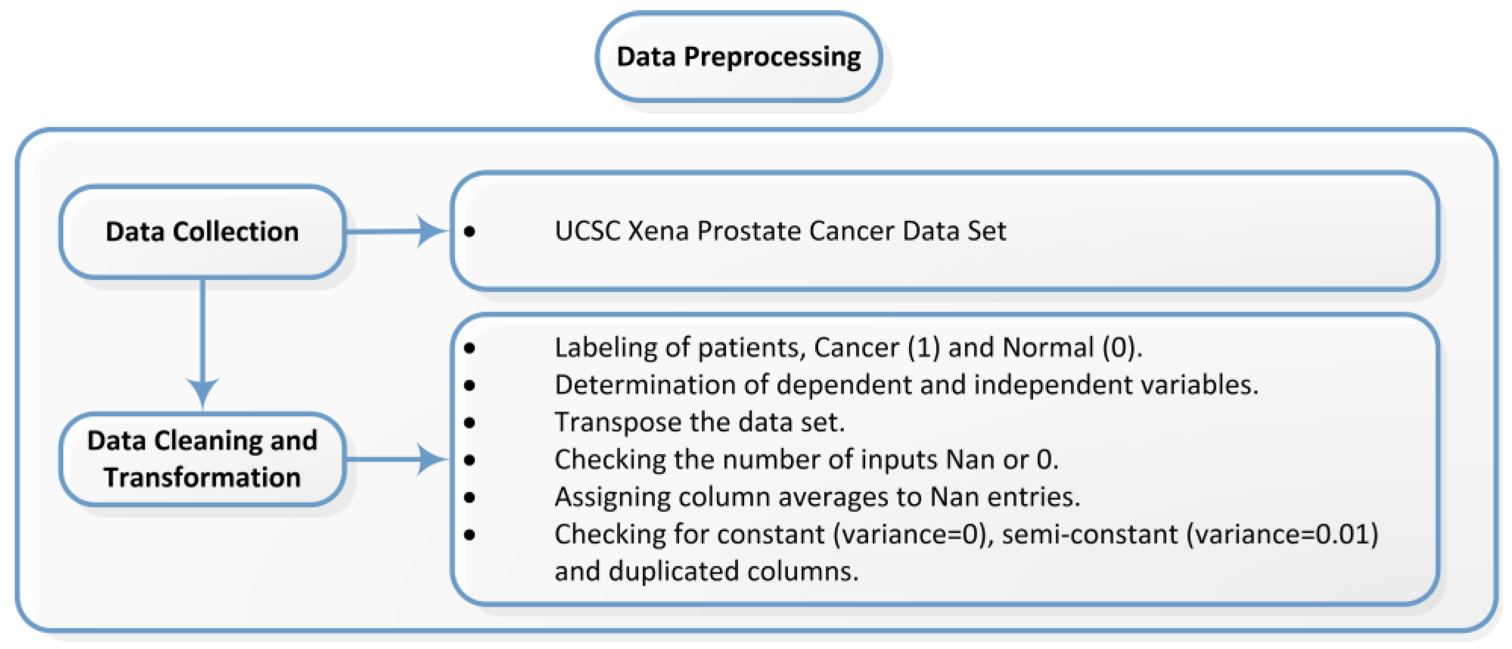
Data pre-processing must be carried out to resolve data issues that would prevent analysis from being performed on the dataset to be analyzed, to interpret the structure of the data, to achieve meaningful data analysis and to extract more meaningful information from the dataset to be applied [30]. Figure 2 shows the basic pre-processing steps performed on the datasets used in the study.

Figure 2. Data pre-processing steps.

For prostate cancer data, the TCGA Prostate Cancer gene expression RNAseq IlluminaHiSeq dataset was obtained from the TCGA Hub at “https://xenabrowser.net/hub/ (accessed on 15 September 2025)”. The RNA sequencing data obtained from UCSC Xena, comprising 498 prostate cancer patients, 52 normal samples (columns) and 20,530 genes (rows), must be labeled as cancer or normal. To obtain the dependent variable, the last two characters of the patient IDs were examined according to the label descriptions in the cancer genome atlas. If the ID fell within the range 01–09, it was labeled as cancer (1) and if within the range 10–19, it was labeled as normal (0). The column header was set to “output”. In the RNA sequencing data, genes are arranged in rows and patients in columns. In the RNA sequencing data, rows and columns were transposed. Subsequently, rows and columns that were unnecessary or not to be used were examined and filtered. The refined genomic dataset consists of 550 samples, one dependent variable indicating the condition of each sample and 17,263 genes.

RNA sequencing datasets were checked for variance, semi-variance and repeated columns. Variance is used to determine how far each number is from the mean and from the other numbers in the set. All observations with a variance less than 0.01 and repeated features have been removed.

The implementation was carried out using python as the programming language within the Anaconda Navigator Spyder development environment. Data analysis was performed with the pandas (2.1.4) library, mathematical and statistical methods were applied using numpy (1.26.3) and scikit-learn (1.6.1) and data visualization was achieved through matplotlib (3.8.2), seaborn (0.13.1), shap (0.48.0) and lime (0.2.0.1).

3.2. Feature Selection Methods

Microarray analysis relies heavily on feature selection, which is the process of finding and eliminating unimportant elements from training data [31]. Filters, wrappers, and embedded methods are the three feature selection techniques that are frequently employed. Filter models choose features without reference to any predictor by using the generic properties of the training data. As part of the selection process, wrapper models optimize a predictor. Embedded methods typically use machine learning models for classification and then the classifier algorithm creates an optimal subset of features [32].

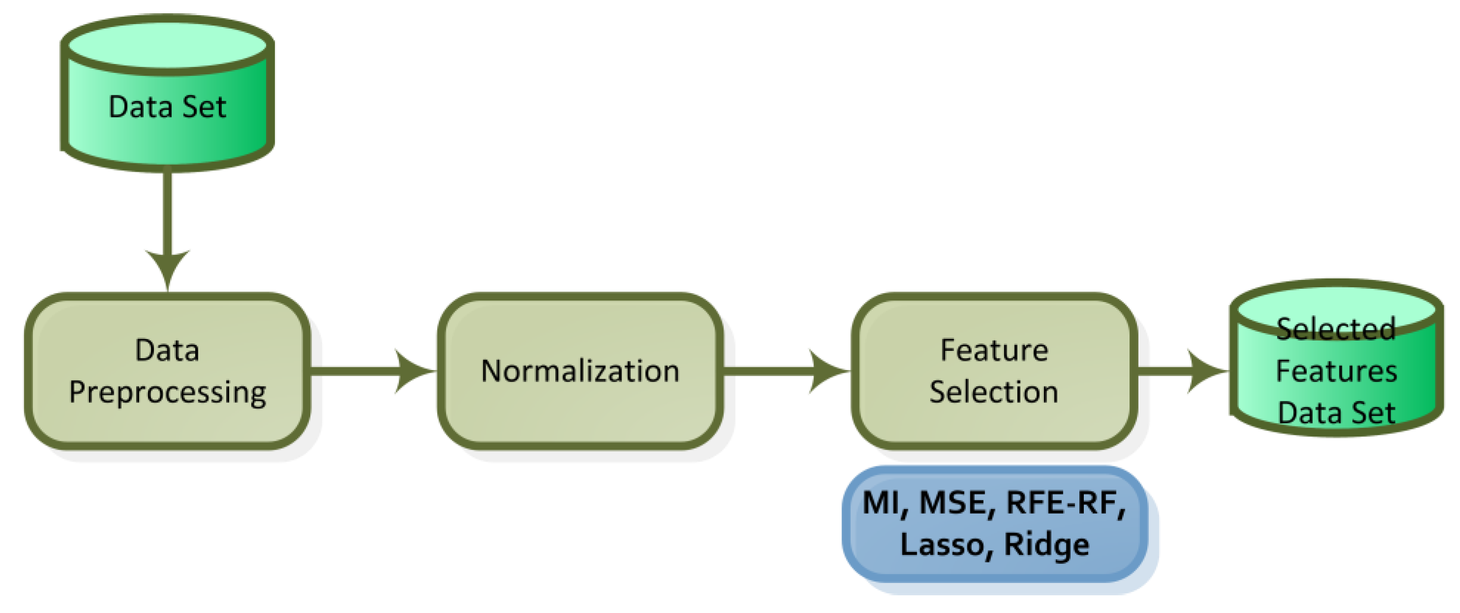
The characteristics in the dataset have a significant impact on a machine learning algorithm’s performance and training time. Redundant features have an impact on the algorithm’s performance in addition to slowing down its training time [33]. In high-dimensional data, feature selection is required to optimize the number of features in order to achieve faster and more accurate classification. The general flowchart of the feature selection performed is provided in Figure 3.

Figure 3. Feature selection flowchart.

By choosing the most significant and helpful characteristics for the problem of interest, feature selection seeks to minimize the number of features in the dataset. Filter, wrapper and embedded methods are commonly used in feature selection.

Five feature selection methods were applied to the datasets: mutual information and mean squared error from the filter methods; recursive feature elimination from the wrapper methods; and Lasso (L1 regularization) and ridge (L2 regularization) from the embedded methods.

Regardless of the model of the machine learning algorithm, filter techniques are a pre-processing step. An evaluation criterion or a score that gauges each feature’s level of relevance to the target variable is used to choose the feature set [34]. Mutual information is a measure of the extent to which knowledge of one variable reduces the uncertainty about another. It measures how much common information two variables share. The mutual information defined by I(X;Y) is expressed in Equation (1). X and Y are two random variables. x and y are the values that random variables can take. P(x, y) represents the joint probability distribution of X = x and Y = y, while p(x) and p(y) represent the marginal probability distributions of X and Y. The larger the result, the stronger the dependency between the two variables [35]. The average of the squares of the variations between actual and expected values is known as mean squared error. If the model contains no error, the MSE equals zero. Its mathematical expression is given by Equation (2). Here, n is the number of observations, ${\mathrm{Y}}_{\mathrm{i}}$ is the actual value, ${\widehat{\mathrm{Y}}}_{\mathrm{i}}$ is the estimated value, and $\left({\mathrm{Y}}_{\mathrm{i}} -{\widehat{\mathrm{Y}}}_{\mathrm{i}}\right)$ represents the estimation error. As the model error increases, the result value also increases.

$$\mathrm{I}\left(\mathrm{X};\mathrm{Y}\right)={\sum }_{\mathrm{x}\in \mathrm{X}}{\sum }_{\mathrm{y}\in \mathrm{Y}}\mathrm{P}\left(\mathrm{x},\mathrm{y}\right)\log {\displaystyle \frac{\mathrm{P}(\mathrm{x},\mathrm{y})}{\mathrm{P}\left(\mathrm{x}\right)\mathrm{P}\left(\mathrm{y}\right)}}$$

(1)

$$\mathrm{MSE}={\displaystyle \frac{1}{\mathrm{n}}} {\sum }_{\mathrm{i}=1}^{\mathrm{n}} {\left({\mathrm{Y}}_{\mathrm{i}} -{\widehat{\mathrm{Y}}}_{\mathrm{i}}\right)}^2$$

(2)

Wrapper methods are feature selection strategies that conduct search operations on the features and assess subsets of features according to the accuracy of a prediction model trained with them [36]. The optimal subset is found by including or excluding variables within the model. RFE aims to achieve high-performance results by eliminating variables of low importance. The elimination process is applied through a machine learning algorithm and by evaluating the results obtained. Based on the results obtained from the applied model, the importance coefficients of the features are calculated and ranked. In this way, the most relevant features can be selected.

Each iteration of the model training process is addressed by embedded methods, which are feature selection strategies and identify the variables that contribute most to training within a specific cycle. Lasso is used for both regularization and model selection. The coefficients of the input variables are penalized. The coefficients of penalized variables are reduced to zero [37]. The mathematical formulation of Lasso is expressed as Equation (3). By including a penalty element, Ridge applies a limit on the coefficients that is comparable to Lasso regression. Ridge regression, on the other hand, takes the square of the coefficients, whereas Lasso regression takes the absolute magnitude. The mathematical formulation of Ridge is expressed as Equation (4). In Equations (3) and (4), n is the number of observations, p is the number of independent variables, ${\mathrm{y}}_{\mathrm{i}}$ and ${ŷ}_{\mathrm{i}}$ are the actual and estimated values, $\left({\mathrm{y}}_{\mathrm{i}}- {ŷ}_{\mathrm{i}}\right)$ is the estimation error, β_j are the feature coefficients, and λ is the penalty coefficient.

$${\mathrm{L}}_{\mathrm{lasso}}\left(\widehat{\mathsf{\beta }}\right)={\sum }_{\mathrm{i}=1}^{\mathrm{n}} {\left({\mathrm{y}}_{\mathrm{i}}- {ŷ}_{\mathrm{i}}\right)}^2+\mathsf{\lambda } {\sum }_{\mathrm{j}=1}^{\mathrm{p}}|{\mathsf{\beta }}_{\mathrm{j}}|$$

(3)

$${\mathrm{L}}_{\mathrm{ridge}}\left(\widehat{\mathsf{\beta }}\right)={\sum }_{\mathrm{i}=1}^{\mathrm{n}} {\left({\mathrm{y}}_{\mathrm{i}}- {ŷ}_{\mathrm{i}}\right)}^2+\mathsf{\lambda } {\sum }_{\mathrm{j}=1}^{\mathrm{p}}{{\mathsf{\beta }}_{\mathrm{j}}}^2$$

(4)

3.3. Machine Learning Algorithms

Data-driven judgments can be made via technologies like deep learning, machine learning, and artificial intelligence. They can be used instead of programming logic in problems that cannot be programmed. Bioinformatic analysis can be performed on patient data using machine learning approaches, which involve data acquisition, pre-processing, normalization or standardization, feature selection or dimensionality reduction, classification, evaluation and survival analysis [38]. Machine learning uses various algorithms that employ iteratively from data to evolve, explain and estimate outcomes [39].

In this study we employed three supervised ML algorithms commonly used in machine learning. Classification was performed using ML algorithms. Subsequently, these algorithms were combined using an ensemble learning model to create a hybrid ensemble learning model.

3.3.1. Traditional Machine Learning Algorithms

In KNN, k neighboring points are examined to define a point. The method is founded on the assumption that nearby points are more likely to share the same label [40]. The most common class among the rows is used to assign a class to the test point and likewise, a class is assigned according to the most successful class among the columns. The optimal K value was determined using the Hamming distance metric with the GridSearchCV() method and calculated with 5-fold cross-validation. Equation (5) is used for the minkowski distance and Equation (6) is used for classification. In Equation (5), n is the vector size, x and y are data points, x_i and y_i are each coordinate, and p is the parameter determining the distance type. In Equation (6), ${\mathrm{y}}_{{\mathrm{k}}_1},{\mathrm{y}}_{{\mathrm{k}}_2},\dots , {\mathrm{y}}_{{\mathrm{k}}_{\mathrm{n}}}$ are the labels of the k nearest neighbors. Predictions are made based on the majority class of the neighbors.

$$\mathrm{D}\left(\mathrm{x}, \mathrm{y}\right)={\left({\sum }_{i=1}^n{{|\mathrm{x}}_{\mathrm{i}}-{\mathrm{y}}_{\mathrm{i}}|}^{\mathrm{p}}\right)}^{1/\mathrm{p}}$$

(5)

$$\widehat{\mathrm{y}}=\mathrm{mod}\left({\mathrm{y}}_{{\mathrm{k}}_1},{\mathrm{y}}_{{\mathrm{k}}_2},\dots , {\mathrm{y}}_{{\mathrm{k}}_{\mathrm{n}}}\right)$$

(6)

Random samples are chosen at random from the dataset in Random Forest. For every sample, a decision tree is constructed in order to produce a forecast outcome. Voting is performed for each predicted result. To determine the optimal option, the prediction result that receives the most votes is chosen as the final prediction result [41].

Samples are represented as points in space by the Support Vector Machine. The samples of distinct categories are mapped to be separated by the widest possible clear margin. The category of new samples is then anticipated by mapping them into the same space and determining which side of the margin they fall into [42]. For data classification, it is necessary to introduce an additional dimension into the feature space. Using Equation (7), the data were mapped into three dimensions for classification that x and y represent the horizontal and vertical dimensions in a two-dimensional plane. In polynomial SVM, the decision function is represented by Equation (8). Here, n is the number of observations, αi are the learned values for each data point, y_i are the labels of the data points, x is the data point, x_i are the training data points, b is the bias term, K(x, x_i) is the kernel function, c is the constant term, and d is the polynomial degree.

$$\mathrm{z}={\mathrm{x}}^2+{\mathrm{y}}^2$$

(7)

$$\mathrm{f}\left(\mathrm{x}\right)={\sum }_{\mathrm{i}=1}^{\mathrm{n}}{\propto }_{\mathrm{i}}{\mathrm{y}}_{\mathrm{i}}\mathrm{K}(\mathrm{x}, {\mathrm{x}}_{\mathrm{i}})+\mathrm{b}, \mathrm{K}(\mathrm{x}, {\mathrm{x}}_{\mathrm{i}})={(\mathrm{x}.{\mathrm{x}}_{\mathrm{i}}+\mathrm{c})}^{\mathrm{d}}$$

(8)

3.3.2. Ensemble Learning

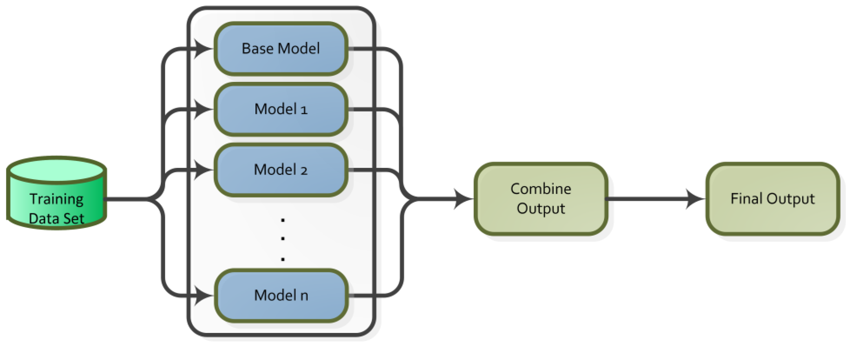
A machine learning technique is ensemble learning that can be applied to enhance classifier performance by combining predictions from multiple models. It is an effective meta-classification technique that increases the effectiveness of weak learners by combining them with strong learners [43]. Ensemble learning operates as a single model according to the working principle in Figure 4 [44].

Figure 4. Ensemble learning flowchart.

There are three fundamental ensemble learning methods: Boosting, Bagging and Stacking. Bagging involves creating multiple training subsets by drawing random samples from the training data. Each subset is used to train multiple models, and the outcomes are aggregated using regression averaging and majority voting for classification. It prevents overfitting and improves the model’s capability to generalize and lowers the variance of the outcomes [44]. Boosting uses subsets generated from the dataset to train models. Models are trained sequentially. New subsets are constructed from misclassified samples. Classification is performed based on the weighted averages of the models. The data is used as input to train several distinct models in stacking. The training results are fed into a meta-classifier, which estimates the weights and predicts the output of each model’s input. The models that perform the best are chosen, and the rest are eliminated [43].

In ensemble learning, several methods exist for selecting appropriate base learners. In the averaging method, the results of the models applied to the dataset are combined and their mean is calculated to determine the class label. In the weighted averaging method, importance weights are assigned to the results of the models. The outcomes are combined by calculating the weighted mean to determine the class label. In the majority voting method, the predictions of the models are listed, and the class label is defined based on the outcome with the highest number of votes. The class label is obtained using the formula ${\mathrm{d}}_{\mathrm{j}} = \mathrm{mode}\{{\mathrm{C}}_1,{\mathrm{C}}_2,\dots ,{\mathrm{C}}_3\}$ [45].

3.3.3. The Proposed Hybrid Ensemble Learning Model

Using the combined strength of ML models to address a learning problem, such a regression or classification matter, is referred to as ensemble learning. Several homogeneous ML models that are considered weak learners are grouped together using this technique. Every weak learner generates its own outcome on either the entire training set or a portion of it, when applied to the issue. Ultimately, the overall result was calculated by combining the outcomes of each weak learner and classification was performed using the majority voting method.

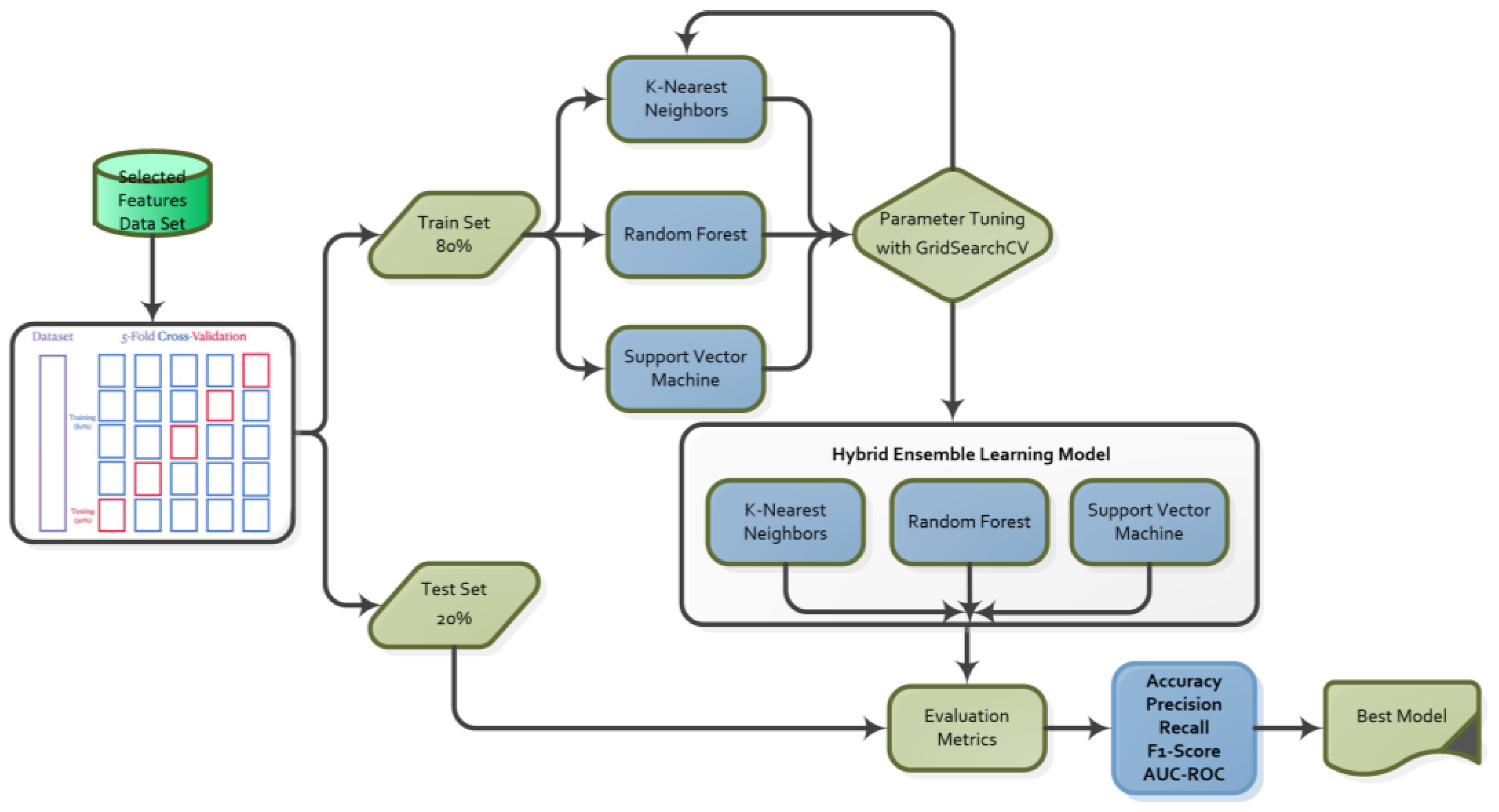
KNN, RF and SVM were used as weak learners to construct a hybrid ensemble learning model, utilizing three categories of models for machine learning. Ensemble models typically employ a homogeneous collection of weak learners. The machine learning algorithms KNN and SVM are not ensemble methods on their own, whereas RF is a bagging method. KNN is a simple yet effective method that can accurately capture local structures, SVM demonstrates strong classification performance on high-dimensional data, and RF prevents the model from overfitting when there are too many features. Furthermore, KNN, RF, and SVM have high performance rates. The combination of these algorithms enables the best modeling of different features, resulting in a robust and reliable hybrid ensemble model using the Majority Voting method. Figure 5 shows the classification and evaluation flowchart for the hybrid community learning model.

Figure 5. Classification and evaluation flowchart.

Filtering, wrapper and embedded methods were used in feature selection. The algorithms commonly used in the literature, namely Mutual Information (MI), Mean Square Error (MSE), Recursive Feature Elimination (RFE), Least Absolute Shrinkage and Selection Operator (Lasso) and Ridge FS, were studied. For each cancer dataset, five separate reduced datasets with 30 variables were obtained according to the parameters set.

Following feature selection, cross-validation was divided the dataset into five subgroups. The ML model’s performance was assessed with cross-validation technique. By performing cross-validation, we ensure that the model generalizes well to unseen data, providing a more reliable estimate of the performance. The primary purpose of cross-validation is to measure the model’s consistency across various data subsets and to reduce the likelihood of overfitting. Five subsets of the dataset are created for 5-fold cross-validation. Each subset is further divided into five parts. One part is used as the test set and the residuals are used as the training set. For each of the five subsets, the roles of training and test data are iteratively shifted, that each part is included in both the training and test data.

The ensemble learning approach in our study is used to combine the predictions of multiple base classifiers (KNN, RF, and SVM) in a majority-voting scheme, which helps to improve the robustness and accuracy of the model. This ensemble method is applied after the feature selection process, where the most relevant features are identified using techniques like Lasso, Ridge, and RFE. Each of the base classifiers is trained on the reduced feature set, and their predictions are aggregated to make the final classification decision. This process ensures that the strengths of each individual classifier are leveraged, enhancing the overall performance.

Cross-validation outputs were provided as input to the k-Nearest Neighbor, Random Forest and Support Vector Machine classifiers. The GridSearchCV method was used when selecting the parameters of the classification algorithms. The GridSearchCV method is a technique that enhances model performance by identifying the optimal hyperparameter combination from a given set of hyperparameter inputs. Hyperparameter optimization is a critical step in improving the performance of machine learning models. The goal of hyperparameter optimization is to identify the optimal combination of hyperparameters that maximizes the model’s accuracy, minimizes the error rate, and enhances the model’s generalizability [46]. Training was conducted using the parameters obtained through hyperparameter optimization with GridSearchCV. To ensure optimal performance, the hyperparameters of the machine learning algorithms used in this study were tuned using GridSearchCV with 5-fold cross-validation. Table 2 summarizes the hyperparameters and their respective values for the K-Nearest Neighbors (KNN), Random Forest (RF), and Support Vector Machine (SVM) models.

Table 2. Hyperparameters for Machine Learning Algorithms.

Classifier	Hyperparameter	Value
KNN	Number of neighbors (k)	7
	Distance metric	minkowski
	Weights	Uniform
RF	Number of trees (n_estimators)	15
	Quality measurement (criterion)	entropy
	Maximum depth (max_depth)	30
	Minimum samples split (min_samples_split)	2
	Minimum samples leaf (min_samples_leaf)	1
SVM	Kernel	poly
	C (regularization parameter)	1.0
	Gamma	Scale
	Probability	True
	Tolerance (tol)	0.001
	Maximum iterations (max_iter)	1000

This table outlines the most relevant hyperparameters for each algorithm, which were selected based on the performance of the model during cross-validation. These parameters were fine-tuned to ensure that each model was optimized for the dataset used in this study.

The outputs of the trained algorithms were combined using the VotingClassifier method to construct the Hybrid Ensemble Learning Model. Visualization was performed using a correlation matrix, which measures the linear relationships among the features in the dataset. Confusion matrices were obtained for the final class prediction results. Results were obtained using evaluation metrics. To validate the results in the prostate cancer dataset, liver, lung and thyroid cancer datasets obtained from the same database were employed. Similar results were obtained for the classification results of other cancer types.

3.4. Evaluation Metrics

One of the performance evaluation methods in classification problems is the confusion matrix. In this study, following the application of each feature selection method and each classification algorithm, the confusion matrix was employed to assess performance, and evaluation metrics specified in Equations (9)–(14) were computed.

Accuracy quantifies, in general, how well the model predicts the correct class across all classes. Precision denotes the success rate of positive predictions. Recall indicates how successfully actual positive cases are identified. The F1 score is the weighted average of precision and recall. AUC projected the model’s capacity to discriminate between classes; for AUC, 0.5 is the threshold value, whereas 1 is the highest value, indicating good classification performance. The Matthews Correlation Coefficient (MCC) provides a more balanced assessment than other metrics such as accuracy, particularly in imbalanced datasets, by utilizing confusion matrix data.

$$\mathrm{Accuracy}={\displaystyle \frac{\left(\mathrm{TP}+\mathrm{TN}\right)}{(\mathrm{TP}+\mathrm{TN}+\mathrm{FP}+\mathrm{FN})}}$$

(9)

$$\mathrm{Precision} ={\displaystyle \frac{\mathrm{TP}}{(\mathrm{TP}+\mathrm{FP})}}$$

(10)

$$\mathrm{Recall}={\displaystyle \frac{\mathrm{TP}}{(\mathrm{TP} +\mathrm{FN})}}$$

(11)

$$\mathrm{F}1 \mathrm{score}= 2 \ast {\displaystyle \frac{(\mathrm{Precision} \ast \mathrm{Recall})}{(\mathrm{Precision}+\mathrm{Recall})}}$$

(12)

$$\mathrm{AUC}={\int }_0^1\mathrm{ROC}\left(\mathrm{t}\right)\mathrm{dt}, \mathrm{ROC}\left(\mathrm{t}\right)={\mathrm{T}}_1\left({\mathrm{T}}_2^{-1}\left(\mathrm{t}\right)\right), \mathrm{t} \mathsf{ϵ} (0,1),$$

(13)

$$\mathrm{MCC}={\displaystyle \frac{\left(\mathrm{TP} \times \mathrm{TN}\right)-(\mathrm{F}\mathrm{P} \times \mathrm{FN})}{\sqrt{(\mathrm{TP}+\mathrm{FP})(\mathrm{TP}+\mathrm{FN})(\mathrm{TN}+\mathrm{FP})(\mathrm{TN}+\mathrm{FN})}}}$$

(14)

4. Results and Discussion

In this study, a hybrid ensemble learning model for feature selection and binary classification on high-dimensional, small-sample prostate cancer RNA-seq gene expression data is presented. The proposed hybrid model was further validated by applying it to lung, liver and thyroid cancer datasets. All RNA-Seq data were obtained from UCSC Xena. Fundamentally, for the prostate, lung, liver and thyroid cancer datasets, pre-processing, feature selection, classification and evaluation were conducted separately and in that order. The procedures described for prostate cancer were likewise applied to the other three cancer datasets. During pre-processing, cancerous and normal samples in the dataset were identified. Samples were labeled based on patient identifiers: if the last two digits were 01–09, the sample was labeled cancer (1); if 10–19, normal (0). The data were checked for the presence of NaN values. By filtering out 3267 genes across 498 prostate cancer and 52 normal samples, the number of genes was reduced from 20,530 to 17,263. Features with variance below 0.01 and duplicate features were removed from the dataset.

In the feature selection stage, five distinct reduced datasets, each comprising 30 variables, were obtained using filter, wrapper and embedded approaches specifically mutual information, mean squared error, recursive feature elimination, the least absolute shrinkage and Lasso and Ridge regression.

Hybrid ensemble learning was created by combining KNN, RF and SVM algorithms with appropriate parameters selected by performing 5-fold cross-validation on the datasets. Results were obtained for each dataset using the majority voting method. Confusion matrices were created for all predictions. Results were obtained using the evaluation metrics. The obtained prostate cancer results were also applied to liver, lung and thyroid cancer datasets, ensuring the accuracy of the proposed method.

The results obtained using four distinct classifiers and five different feature selection methods were presented comparatively in Table 3 and Figure 6. When the proposed hybrid ensemble method was employed with Lasso-based feature selection, the highest accuracy of 0.9782, F1-score of 0.9880 and AUC of 0.9865 were achieved.

Table 3. Prostate cancer classification results.

Classifier	Feature Selectors	Accuracy	Precision	Recall	F1-Score	AUC-ROC	MCC
KNN	MI	0.9636	0.9803	0.9799	0.9799	0.9340	0.7993
	MSE	0.9545	0.9707	0.9799	0.9752	0.9412	0.7773
	RFE by RF	0.9673	0.9768	0.9879	0.9822	0.9494	0.7941
	Lasso	0.9745	0.9844	0.9879	0.9861	0.9661	0.8130
	Ridge	0.9436	0.9467	0.9939	0.9697	0.8888	0.6736
RF	MI	0.9618	0.9692	0.9899	0.9793	0.9637	0.7738
	MSE	0.9545	0.9673	0.9839	0.9753	0.9654	0.7695
	RFE by RF	0.9582	0.9672	0.9879	0.9774	0.9605	0.7899
	Lasso	0.9673	0.9750	0.9899	0.9822	0.9652	0.8028
	Ridge	0.9309	0.9389	0.9880	0.9628	0.9261	0.6437
SVM	MI	0.9436	0.9702	0.9679	0.9690	0.9290	0.7320
	MSE	0.9545	0.9726	0.9778	0.9750	0.9579	0.7698
	RFE by RF	0.9600	0.9747	0.9818	0.9781	0.9707	0.7699
	Lasso	0.9727	0.9879	0.9818	0.9848	0.9897	0.8043
	Ridge	0.9109	0.9612	0.9397	0.9502	0.9206	0.6011
Proposed Hybrid Ensemble Method	MI	0.9655	0.9712	0.9920	0.9813	0.9735	0.8217
	MSE	0.9582	0.9711	0.9839	0.9772	0.9769	0.7775
	RFE by RF	0.9673	0.9732	0.9919	0.9823	0.9878	0.8030
	Lasso	0.9782	0.9862	0.9899	0.9880	0.9868	0.8589
	Ridge	0.9309	0.9356	0.9919	0.9629	0.9433	0.6983

Figure 6. Prostate cancer classification results according to feature selection methods.

When the base classifiers are examined, the SVM with Lasso-based feature selection achieved an accuracy of 0.9727 and an AUC of 0.9897. RF exhibited balanced performance across different feature selection methods, with its best results again obtained using Lasso. Although KNN has an interpretable operating mechanism, when combined with Lasso feature selection it delivered strong performance 0.9745 accuracy and an F1-score of 0.9861 yet it still fell short of the proposed hybrid ensemble method.

The Matthews Correlation Coefficient (MCC) values provide a more comprehensive measure of model performance, especially in the presence of imbalanced data. As seen in the table, the Hybrid Ensemble model consistently outperforms other classifiers across all feature selection methods, achieving the highest MCC values, particularly with Lasso (0.8589) and RFE (0.8031). This indicates that the ensemble method, by combining multiple classifiers, improves the model’s ability to handle both positive and negative class predictions effectively. In contrast, Ridge feature selection consistently yields the lowest MCC values across all models, suggesting that L2 regularization alone is less effective in selecting discriminative features in imbalanced datasets. KNN, RF, and SVM show comparable MCC values, with slight variations depending on the feature selection method used, demonstrating that while they perform well, they do not match the hybrid ensemble in terms of overall classification stability and balance. These MCC values confirm that ensemble methods, particularly with Lasso-based feature selection, offer significant advantages in terms of handling imbalanced data and improving model generalizability.

Evaluated in terms of feature selection methods, Lasso yielded the best results across all classifiers. By imposing an L1 regularization penalty, less significant characteristics’ coefficients were reduced to zero by Lasso, thereby removing irrelevant or redundant variables from the dataset and improving the model’s generalizability. It was observed that the MI based feature selection method did not provide sufficiently strong discrimination with some classifiers. Using MSE criterion, the best result 0.9582 was obtained with the proposed method; however, overall, it exhibited relatively weak performance in distinguishing among different models. RFE approach achieved high performance with both the proposed hybrid ensemble learner and SVM, emerging as a viable alternative to Lasso. By contrast, Ridge displayed the weakest performance across all classifiers, indicating that L2 regularization alone is insufficient for selecting discriminative features.

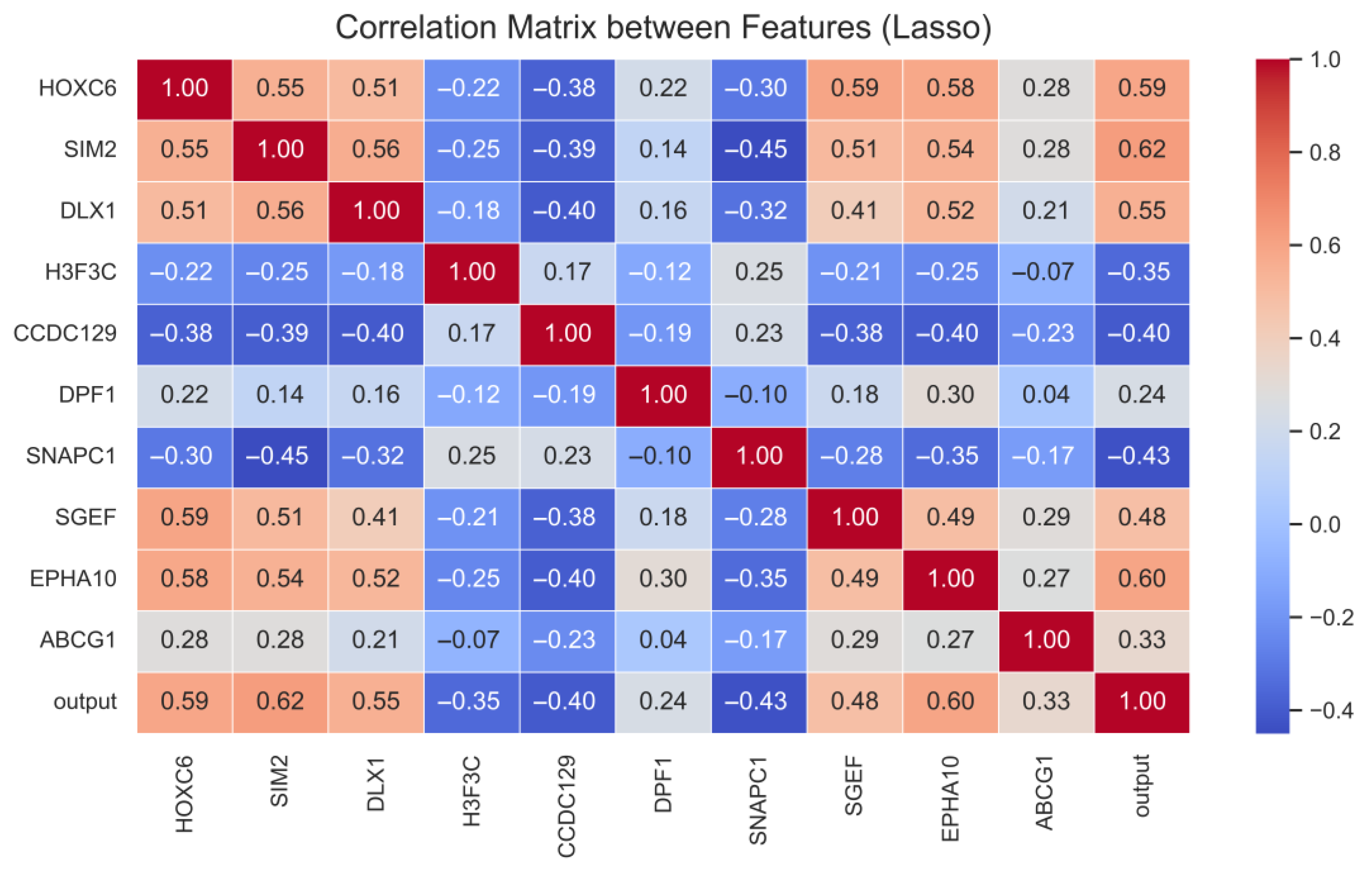
Figure 7 illustrates the linear relationships among the expression values of genes identified via Lasso-based feature selection. Only the more important features have been used in the visual to make the correlation matrix understandable. In the matrix, red tones denote positive correlations, whereas blue tones indicate negative correlations. Moderate-to-high correlations were observed for the gene pairs HOXC6–SIM2, HOXC6–DLX1 and EPHA10–HOXC6, suggesting that these pairs may share similar regulatory mechanisms in biological processes. For most genes, the correlation structure indicates that the features carry largely independent information, minimizing the risk of exceedingly strong associations between any two variables. Significant positive correlations were observed between the independent variable and the genes HOXC6 (r = 0.59), SIM2 (r = 0.62), DLX1 (r = 0.55) and EPHA10 (r = 0.60). These genes emerge as candidate biomarkers contributing most to classification performance.

Figure 7. Prostate cancer Lasso correlation results.

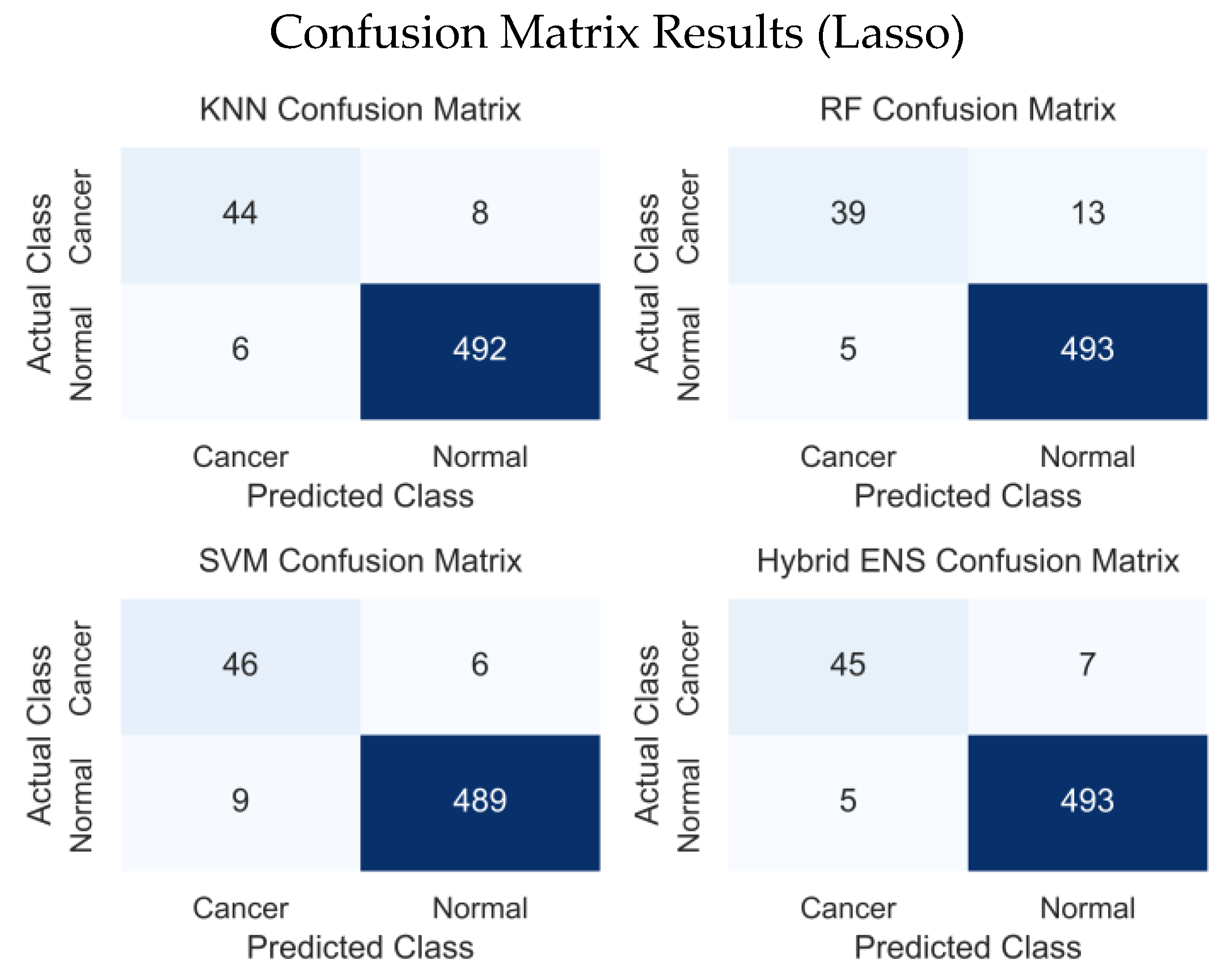
Figure 8 presents the confusion-matrix results for KNN, RF, SVM and Hybrid Ensemble models. In comparison, KNN made 6 misclassifications among normal samples and 8 among cancerous samples, yielding a balanced performance but with sensitivity that was relatively lower than SVM. RF misclassified 5 normal and 13 cancerous samples, performing slightly worse than KNN and SVM in correctly identifying cancer cases. SVM misclassified 9 normal and 6 cancerous samples, achieving the highest sensitivity for the cancer class. The proposed hybrid ensemble misclassified 5 normal and 7 cancerous samples 12 in total thus providing the most balanced performance overall. These results indicate that the proposed hybrid model offers more stable predictions and stronger generalization capability than the individual models.

Figure 8. Prostate cancer Lasso confusion matrix results.

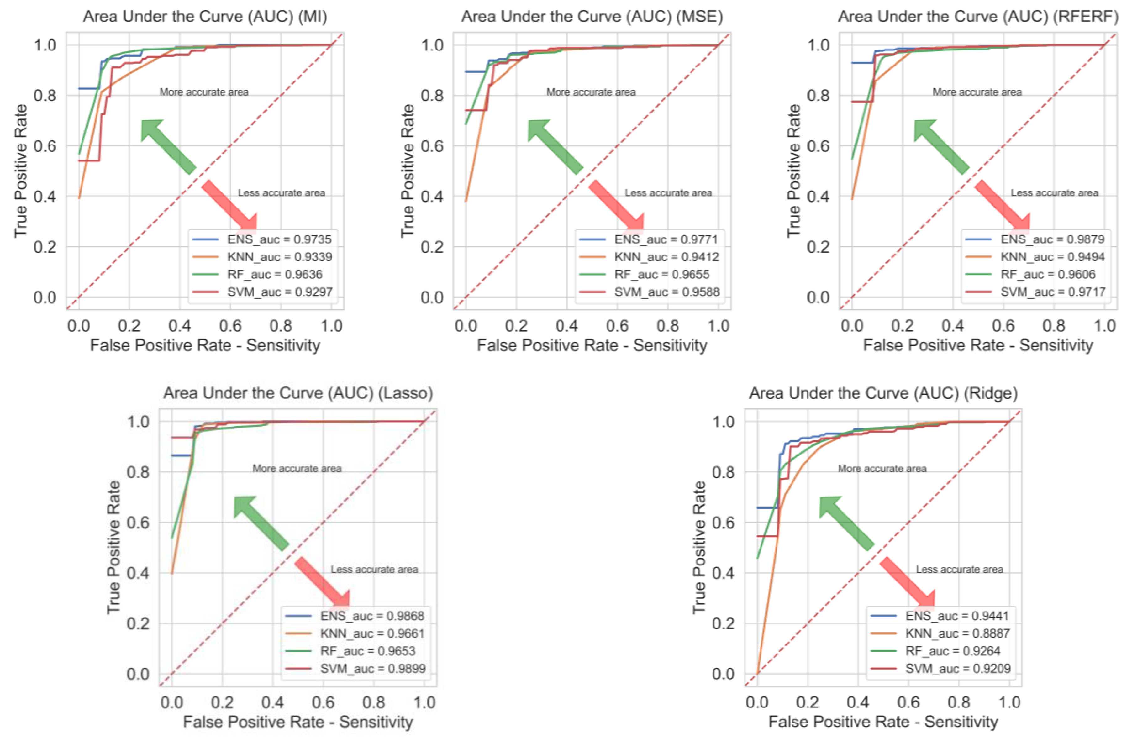
The impact of feature selection methods on classification outcomes is depicted in Figure 9 through ROC curves and their corresponding AUC values. AUC quantifies the classifier’s ability to discriminate between classes: values approaching 1 indicate stable and reliable classification, whereas an AUC of 0.5 denotes an uninformative classifier (no better than chance). Overall, the proposed hybrid model achieved the highest AUC across the four feature selection methods. Moreover, it delivered consistent and strong performance in minimizing generalization error among different feature selection methods.

Figure 9. Prostate cancer area under the curve results.

XAI techniques are used to prevent the negative effects of automated decision-making processes in feature selection, to help make more informed choices and to reveal and protect potential security vulnerabilities [47]. SHAP and LIME are two widely used XAI methods. These two methods propose a framework for interpreting the outputs, highlighting their strengths and weaknesses.

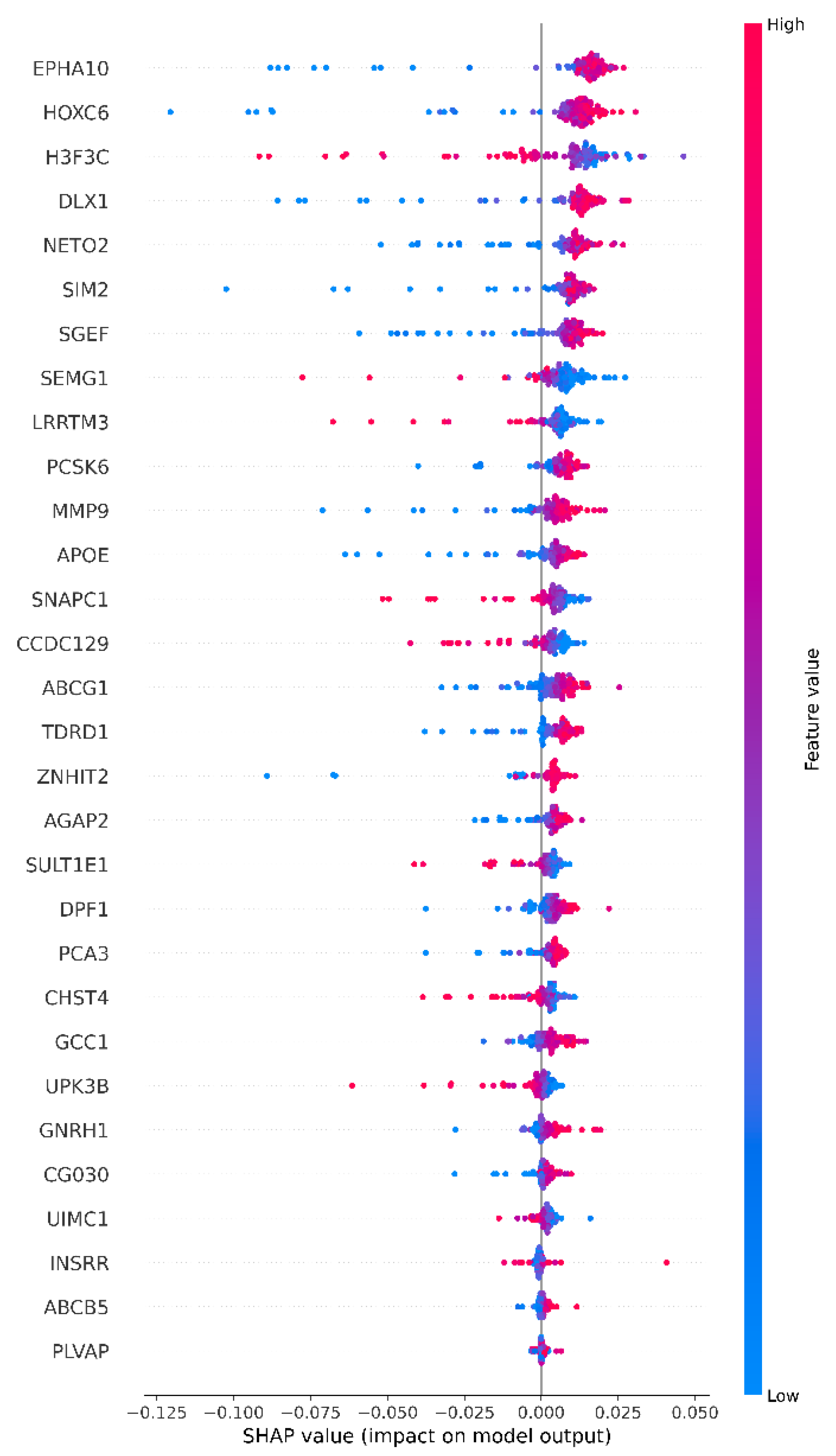
The SHAP beeswarm plot summarizes the variables that influence model output at a global level. Features are ranked from top to bottom according to the average SHAP value, with the horizontal axis representing the marginal contribution for each sample. Colors encode feature values; dark pink represents high, blue represents low. A SHAP plot summarizing which variables influence the model’s Class-1 decision, in what direction and to what extent, is shown in Figure 10.

Figure 10. Prostate cancer Lasso XAI SHAP results.

EPHA10 and HOXC6 are the most dominant predictors in selecting cancerous samples. High values mostly shift to the right, increasing model output, while low values shift to the left, decreasing it. The reverse pattern is observed for H3F3C. In other words, it is decisive in choosing normal examples. High values are heavily weighted to the left, suppressing output, while low values partially shift it to the right. While high values in SEMG1, PCSK6, MMP9 and partially in APOE, SNAPC1 and CCDC129 produce a positive effect, high values in some variables, such as ABCG1 and DPF1, tend to have a negative effect For some features, such as NETO2 and LRRTM3, the scattering of points both to the right and left suggests that the effect may be sensitive to context and interactions. In general, longer tails on the left indicate that the negative effect may be stronger in some samples, while the top variables drive the model decision in terms of both effect size and between-sample variability [48,49].

LIME is a model-agnostic method developed to generate local explanations for individual predictions of machine learning models. LIME generates synthetic perturbations in the vicinity of the sample studied and forces the main model to predict these examples. It then trains an interpretable surrogate model on data weighted by distance from the sample, extracting the feature contributions that best explain the prediction [50]. The model-agnostic nature of the LIME method enables it to be applied to various machine learning models, making it flexible across a wide range of use cases. LIME can help increase trust in AI systems by transparently explaining the decision-making process behind predictions, particularly in critical areas such as healthcare [51].

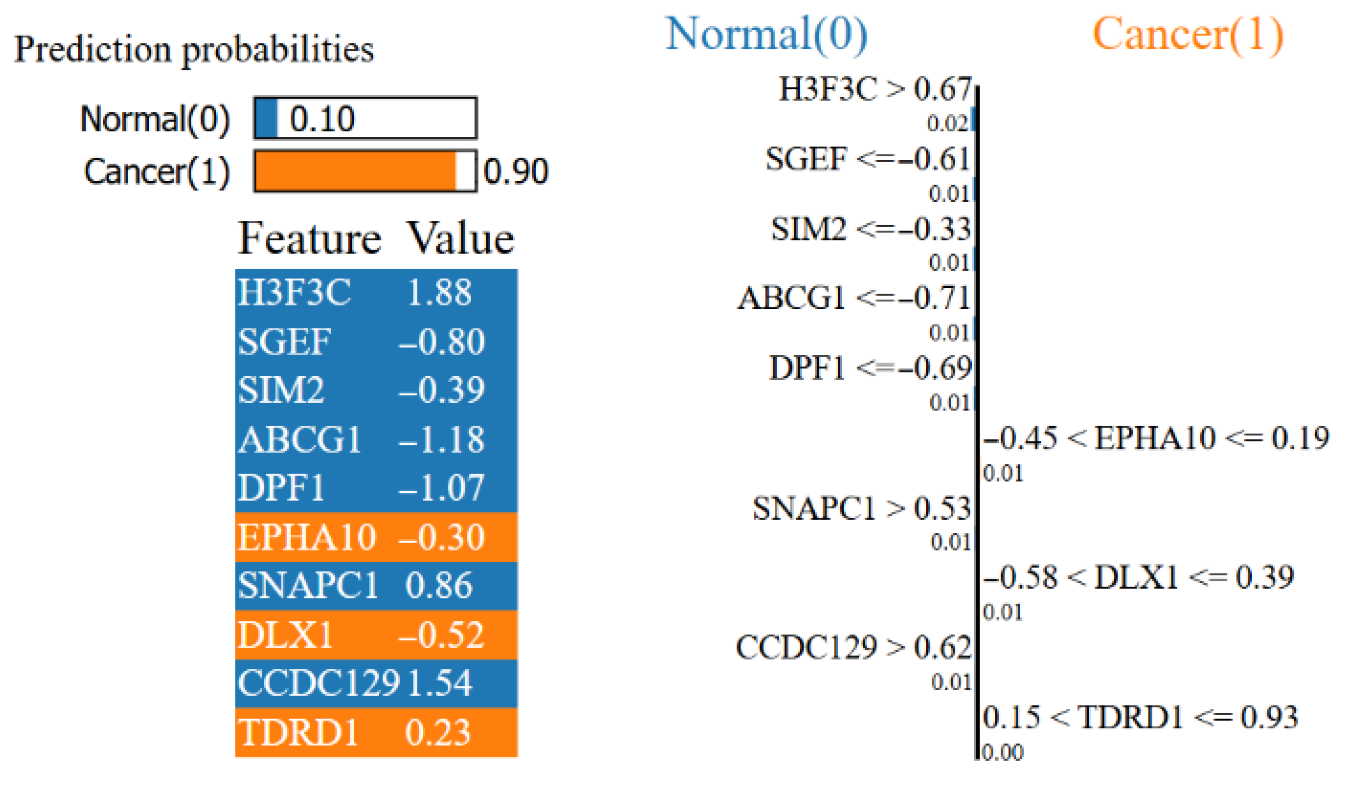
Figure 11 shows that the model gives a 90% probability of cancer and a 10% probability of Normal and which features drove this decision. The orange features on the right represent local contributions supporting the cancer classification. The high values of SNAPC1 and CCDC129, along with the range of EPHA10 and DLX1, push this sample toward cancer. The blue features on the left, H3F3C, SGEF, SIM2, ABCG1 and DPF1, favor normal classification. While the relatively high H3F3C and low levels of SGEF, ABCG1 and DPF1 favor normal, their combined contributions are insufficient to offset the opposite. The direction of the bars indicates the class to which the contribution is directed, and the length indicates its local weight. The numbers in the table represent the standardized values of the relevant feature in this example. As a result, although there are signals supporting normal, the model classifies this sample as cancer due to the dominant local indicators in favor of cancer.

Figure 11. Prostate cancer Lasso XAI LIME results.

According to the results derived from the correlation matrix and the XAI methods SHAP and LIME, the genes EPHA10, HOXC6, DLX1, H3F3C, ABCG1 and DPF1 were effective in discriminating cancerous from normal samples. Among the genes proposed by the model that are particularly effective for classifying cancer cases, EPHA10 is a element of the Eph receptor tyrosine kinase family. It is emerging as a functionally important pseudokinase that contributes to cellular signaling and multiple aspects of tumor biology. Aberrant expression of EPHA10 is also implicated in prostate, breast and colon cancers. Consequently, targeting EPHA10 may confer therapeutic benefits across multiple tumor types [52]. All multicellular organisms’ morphogenesis depends on the highly conserved transcription factors encoded by the homeobox family, of which HOXC6 is a member [53]. DLX1 plays an important role during neurodevelopment. The encoded protein might be involved in the differentiation and survival of inhibitory neurons in the forebrain as well as the regulation of craniofacial patterning [54]. Chromatin incorporation of H3F3C histone variants, which are effective in classifying normal samples, also plays an important role in establishing specific chromatin states [55]. ABCG1 is a regulator of macrophage cholesterol and phospholipid transport [56]. DPF1 is associated with both chromatin remodeling and essential regulatory processes in early embryonic development and enhanced chemoreception [57].

The effectiveness of the suggested approach on the prostate cancer dataset was validated using liver, lung and thyroid cancer datasets from the same database. The classification performance achieved by the proposed model for four different cancer datasets is reported in Table 4 and the results are examined.

Table 4. Comparison of classification results.

Classifier	Feature Selection	Dataset	Accuracy	Precision	Recall	F1-Score	AUC-ROC
Proposed Hybrid Ensemble Method	Lasso	LIHC	0.9976	1.0000	0.9972	0.9986	1.000
		LUNG	0.9965	0.9981	0.9981	0.9981	0.9997
		THCA	0.9948	0.9980	0.9961	0.9971	0.9990
		PRAD	0.9782	0.9862	0.9899	0.9880	0.9868

The results of our study indicate that Lasso (L1 regularization) is a more effective feature selector than Ridge (L2 regularization). This can be explained by the differing properties of L1 and L2 regularization. Lasso regularization induces sparsity in the model by shrinking some feature coefficients to exactly zero, effectively excluding irrelevant or redundant features from the model. This characteristic makes Lasso particularly advantageous in high-dimensional datasets, such as genomic data, where many features (genes) may not contribute significantly to the classification task. In contrast, Ridge regularization only reduces the magnitude of coefficients but does not set any coefficients to zero, meaning that all features are retained, albeit with smaller coefficients. As a result, Ridge is less effective in feature selection, especially when the dataset contains a large number of irrelevant features. This theoretical distinction between Lasso and Ridge helps explain why Lasso outperforms Ridge in our experiments.

While this study presents promising results, several limitations should be acknowledged. The dataset used is relatively small and imbalanced, which may affect the generalizability of the results. Additionally, while we employed multiple feature selection techniques, there are other advanced methods that could potentially improve model performance. Although external validation was performed on datasets from different cancer types, further validation with more diverse real-world clinical data is needed. The interpretability of ensemble methods, especially those combining multiple classifiers, remains a challenge, and the computational cost of training these models can be high. These limitations highlight areas for future work, including expanding the dataset, exploring additional feature selection methods, and improving scalability and interpretability.

An examination of the results reveals minor differences; nevertheless, they are important for evaluating the generalizability of the proposed model across different datasets. The fact that all metrics obtained in the prostate dataset are above 97% reveals that the model generally demonstrates high success and has strong classification ability. Although the performance values are slightly lower than other datasets, these differences do not indicate a significant weakness in the success of the model. On the contrary, the distribution of performance on different datasets confirms that the generalizability of the model is high. This demonstrates that the model operates robustly and reliably even on datasets with differing biological and molecular characteristics.

5. Conclusions

Our aim in this study is to provide an effective model for classifying high-dimensional, small-sample prostate cancer RNA sequencing gene expression data. We suggest a framework for hybrid ensemble learning that incorporates several feature selection techniques with machine learning algorithms. Specifically, the model employs hybrid ensembles formed by combining feature selection methods MI, MSE, RFE, Lasso and Ridge with KNN, RF and SVM classifiers.

The results indicate that the proposed hybrid ensemble learning model outperforms conventional classifiers. Among the feature selection methods, Lasso generally emerged as the most effective, whereas Ridge was the weakest. With Lasso-based feature selection, the proposed hybrid ensemble model achieved strong performance across the primary metrics, attaining an accuracy of 0.9782, precision of 0.9862, recall of 0.9899, F1 score of 0.9880 and an AUC of 0.9868.

To interpret the selected features, SHAP and LIME methods within explainable AI, along with correlation analyses, were employed. The resulting visualizations reveal that high expression levels of EPHA10, HOXC6 and DLX1 directly contribute to the successful classification of cancerous samples, whereas high H3F3C and low ABCG1 and DPF1 expression levels directly aid in the classification of normal samples.

In conclusion, by integrating the strengths of diverse classifiers, the proposed hybrid ensemble learning model yields a more stable, reliable and generalizable framework that delivers high classification performance across multiple cancer types. The findings obtained substantiate this claim. Based on the findings of this study, one focus area for future research could be a more in-depth examination of the interactions between genes identified using XAI methods. Investigating multi-stage feature selection strategies to further optimize gene selection processes may be beneficial for improving the model’s accuracy and generalization ability. Such studies may contribute to a better understanding of biologically meaningful genes and make the model more suitable for clinical applications. Moreover, the approach makes notable contributions to both bioinformatics and machine learning. The proposed method offers a robust alternative for analyzing small sample sizes and high-dimensional gene expression data and is considered an extensible strategy that can be expanded to support early cancer diagnosis. Future work may further enhance its generalizability by applying the model to additional cancer types and real-world clinical datasets.

References

1. Sung, H.; Ferlay, J.; Siegel, R.L.; Laversanne, M.; Soerjomataram, I.; Jemal, A.; Bray, F. Global Cancer Statistics 2020: GLOBOCAN Estimates of Incidence and Mortality Worldwide for 36 Cancers in 185 Countries. CA Cancer J. Clin. 2021, 71, 209–249. [Google Scholar] [CrossRef]
2. James, N.D.; Tannock, I.; N’Dow, J.; Feng, F.; Gillessen, S.; Ali, S.A.; Trujillo, B.; Al-Lazikani, B.; Attard, G.; Bray, F.; et al. The Lancet Commission on Prostate Cancer: Planning for the Surge in Cases. Lancet 2024, 403, 1683–1722. [Google Scholar] [CrossRef]
3. Hong, M.; Tao, S.; Zhang, L.; Diao, L.T.; Huang, X.; Huang, S.; Xie, S.J.; Xiao, Z.D.; Zhang, H. RNA Sequencing: New Technologies and Applications in Cancer Research. J. Hematol. Oncol. 2020, 13, 166. [Google Scholar] [CrossRef]
4. Giganti, F.; Moreira da Silva, N.; Yeung, M.; Davies, L.; Frary, A.; Ferrer Rodriguez, M.; Sushentsev, N.; Ashley, N.; Andreou, A.; Bradley, A.; et al. AI-Powered Prostate Cancer Detection: A Multi-Centre, Multi-Scanner Validation Study. Eur. Radiol. 2025, 35, 4915–4924. [Google Scholar] [CrossRef]
5. Saha, A.; Bosma, J.S.; Twilt, J.J.; van Ginneken, B.; Bjartell, A.; Padhani, A.R.; Bonekamp, D.; Villeirs, G.; Salomon, G.; Giannarini, G.; et al. Artificial Intelligence and Radiologists in Prostate Cancer Detection on MRI (PI-CAI): An International, Paired, Non-Inferiority, Confirmatory Study. Lancet Oncol. 2024, 25, 879–887. [Google Scholar] [CrossRef]
6. Teke, M.; Etem, T. Cascading GLCM and T-SNE for Detecting Tumor on Kidney CT Images with Lightweight Machine Learning Design. Eur. Phys. J. Spec. Top. 2025, 1–16. [Google Scholar] [CrossRef]
7. Goldenberg, S.L.; Nir, G.; Salcudean, S.E. A New Era: Artificial Intelligence and Machine Learning in Prostate Cancer. Nat. Rev. Urol. 2019, 16, 391–403. [Google Scholar] [CrossRef] [PubMed]
8. Jain, A. Feature Selection: Evaluation, Application, and Small Sample Performance. IEEE Trans. Pattern Anal. Mach. Intell. 1997, 19, 153–158. [Google Scholar] [CrossRef]
9. Golub, T.R.; Slonim, D.K.; Tamayo, P.; Huard, C.; Gaasenbeek, M.; Mesirov, J.P.; Coller, H.; Loh, M.L.; Downing, J.R.; Caligiuri, M.A.; et al. Molecular Classification of Cancer: Class Discovery and Class Prediction by Gene Expression Monitoring. Science 1999, 286, 531–537. [Google Scholar] [CrossRef]
10. Berrar, D.; Bradbury, I.; Dubitzky, W. Avoiding Model Selection Bias in Small-Sample Genomic Datasets. Bioinformatics 2006, 22, 1245–1250. [Google Scholar] [CrossRef] [PubMed]
11. Goldman, M.; Craft, B.; Hastie, M.; Repečka, K.; McDade, F.; Kamath, A.; Banerjee, A.; Luo, Y.; Rogers, D.; Brooks, A.N.; et al. The UCSC Xena Platform for Public and Private Cancer Genomics Data Visualization and Interpretation. bioRxiv 2019. bioRxiv:326470. [Google Scholar] [CrossRef]
12. Dhumkekar, A.A.; Ghorpade, S.; Awale, R.N. Performance Analysis of Various Cancers Using Genetic Data with Variance Threshold. In Proceedings of the 2022 OITS International Conference on Information Technology (OCIT), Bhubaneswar, India, 14–16 December 2022; IEEE: New York, NY, USA, 2022; pp. 67–72. [Google Scholar] [CrossRef]
13. Shamsara, E.; Shamsara, J. Bioinformatics Analysis of the Genes Involved in the Extension of Prostate Cancer to Adjacent Lymph Nodes by Supervised and Unsupervised Machine Learning Methods: The Role of SPAG1 and PLEKHF2. Genomics 2020, 112, 3871–3882. [Google Scholar] [CrossRef]
14. Begum, S.; Sarkar, R.; Chakraborty, D.; Sen, S.; Maulik, U. Application of Active Learning in DNA Microarray Data for Cancerous Gene Identification. Expert Syst. Appl. 2021, 177, 114914. [Google Scholar] [CrossRef]
15. Gumaei, A.; Sammouda, R.; Al-Rakhami, M.; AlSalman, H.; El-Zaart, A. Feature Selection with Ensemble Learning for Prostate Cancer Diagnosis from Microarray Gene Expression. Health Inform. J. 2021, 27, 1460458221989402. [Google Scholar] [CrossRef]
16. Fathi, H.; AlSalman, H.; Gumaei, A.; Manhrawy, I.I.M.; Hussien, A.G.; El-Kafrawy, P. An Efficient Cancer Classification Model Using Microarray and High-Dimensional Data. Comput. Intell. Neurosci. 2021, 2021, 7231126. [Google Scholar] [CrossRef]
17. He, B.; Zhang, Y.; Zhou, Z.; Wang, B.; Liang, Y.; Lang, J.; Lin, H.; Bing, P.; Yu, L.; Sun, D.; et al. A Neural Network Framework for Predicting the Tissue-of-Origin of 15 Common Cancer Types Based on RNA-Seq Data. Front. Bioeng. Biotechnol. 2020, 8, 737. [Google Scholar] [CrossRef]
18. Santo, G.D.; Frasca, M.; Bertoli, G.; Castiglioni, I.; Cava, C. Identification of Key MiRNAs in Prostate Cancer Progression Based on MiRNA-MRNA Network Construction. Comput. Struct. Biotechnol. J. 2022, 20, 864–873. [Google Scholar] [CrossRef] [PubMed]
19. Senbagamalar, L.; Logeswari, S. Genetic Clustering Algorithm-Based Feature Selection and Divergent Random Forest for Multiclass Cancer Classification Using Gene Expression Data. Int. J. Comput. Intell. Syst. 2024, 17, 23. [Google Scholar] [CrossRef]
20. Razzaque, A.; Badholia, D.A. PCA Based Feature Extraction and MPSO Based Feature Selection for Gene Expression Microarray Medical Data Classification. Meas. Sens. 2024, 31, 100945. [Google Scholar] [CrossRef]
21. Venkataramana, L.; Jacob, S.G.; Saraswathi, S.; Venkata Vara Prasad, D. Identification of Common and Dissimilar Biomarkers for Different Cancer Types from Gene Expressions of RNA-Sequencing Data. Gene Rep. 2020, 19, 100654. [Google Scholar] [CrossRef]
22. Yaping, Z.; Changyin, Z. Gene Feature Selection Method Based on ReliefF and Pearson Correlation. In Proceedings of the 2021 3rd International Conference on Applied Machine Learning (ICAML), Changsha, China, 23–25 July 2021; IEEE: New York, NY, USA, 2021; pp. 15–19. [Google Scholar] [CrossRef]
23. Ali, N.M.; Hanafi, A.N.; Karis, M.S.; Shamsudin, N.H.; Shair, E.F.; Abdul Aziz, N.H. Hybrid Feature Selection of Microarray Prostate Cancer Diagnostic System. Indones. J. Electr. Eng. Comput. Sci. 2024, 36, 1884. [Google Scholar] [CrossRef]
24. Bhonde, S.B.; Wagh, S.K.; Prasad, J.R. Identification of Cancer Types from Gene Expressions Using Learning Techniques. Comput. Methods Biomech. Biomed. Eng. 2023, 26, 1951–1965. [Google Scholar] [CrossRef]
25. Mostavi, M.; Chiu, Y.C.; Huang, Y.; Chen, Y. Convolutional Neural Network Models for Cancer Type Prediction Based on Gene Expression. BMC Med. Genomics 2020, 13, 44. [Google Scholar] [CrossRef]
26. Petinrin, O.O.; Saeed, F.; Salim, N.; Toseef, M.; Liu, Z.; Muyide, I.O. Dimension Reduction and Classifier-Based Feature Selection for Oversampled Gene Expression Data and Cancer Classification. Processes 2023, 11, 1940. [Google Scholar] [CrossRef]
27. Alkhanbouli, R.; Matar Abdulla Almadhaani, H.; Alhosani, F.; Simsekler, M.C.E. The Role of Explainable Artificial Intelligence in Disease Prediction: A Systematic Literature Review and Future Research Directions. BMC Med. Inform. Decis. Mak. 2025, 25, 110. [Google Scholar] [CrossRef]
28. Antunes, M.E.; Araújo, T.G.; Till, T.M.; Pantaleão, E.; Mancera, P.F.A.; de Oliveira, M.H. Machine Learning Models for Predicting Prostate Cancer Recurrence and Identifying Potential Molecular Biomarkers. Front. Oncol. 2025, 15, 1535091. [Google Scholar] [CrossRef]
29. The Cancer Genome Atlas Program (TCGA)—NCI. Available online: https://www.cancer.gov/ccg/research/genome-sequencing/tcga (accessed on 6 September 2025).
30. Oğuzlar, A. Veri Ön İşleme. Erciyes Üniv. İktisadi ve İdari Bilim. Fakültesi Derg. 2003, 21, 67–76. Available online: https://dergipark.org.tr/tr/pub/erciyesiibd/issue/5878/77794 (accessed on 8 October 2025).
31. Feature Extraction: Foundations and Applications—Google Kitaplar. Available online: https://books.google.com.tr/books?hl=tr&lr=&id=FOTzBwAAQBAJ&oi=fnd&pg=PA1&dq=Feature+Extraction:+Foundations+and+Applications&ots=5Vj9N4aokV&sig=oialtKbQKDqW869D9Ts2LrH7DvA&redir_esc=y#v=onepage&q=Feature%20Extraction%3A%20Foundations%20and%20Applications&f=false (accessed on 7 January 2025).
32. Bolón-Canedo, V.; Sánchez-Maroño, N.; Alonso-Betanzos, A.; Benítez, J.M.; Herrera, F. A Review of Microarray Datasets and Applied Feature Selection Methods. Inf. Sci. 2014, 282, 111–135. [Google Scholar] [CrossRef]
33. Applying Filter Methods in Python for Feature Selection. Available online: https://stackabuse.com/applying-filter-methods-in-python-for-feature-selection/ (accessed on 7 January 2025).
34. Landset, S.; Khoshgoftaar, T.M.; Richter, A.N.; Hasanin, T. A Survey of Open Source Tools for Machine Learning with Big Data in the Hadoop Ecosystem. J. Big Data 2015, 2, 24. [Google Scholar] [CrossRef]
35. Novaković, J.; Strbac, P.; Bulatović, D. Toward Optimal Feature Selection Using Ranking Methods and Classification Algorithms. Yugosl. J. Oper. Res. 2011, 21, 119–135. [Google Scholar] [CrossRef]
36. Kushmerick, N.; Weld, D.S.; Doorenbos, R.B. Wrapper Induction for Information Extraction. Int. Jt. Conf. Artif. Intell. 1997, 1, 729–735. Available online: https://api.semanticscholar.org/CorpusID:5119155 (accessed on 8 October 2025).
37. Makine Öğrenmesinde Değişken Seçimi (Feature Selection) Yazı Serisi: Gömülü (Embedded) Yöntemler ve Python Kodları by Yiğit Şener Medium. Available online: https://yigitsener.medium.com/makine-%C3%B6%C4%9Frenmesinde-de%C4%9Fi%C5%9Fken-se%C3%A7imi-feature-selection-yaz%C4%B1-serisi-g%C3%B6m%C3%BCl%C3%BC-embedded-y%C3%B6ntemler-c23293915b39 (accessed on 7 January 2025).
38. Aydın Atasoy, N.; Demiröz, A. Makine Öğrenmesi Algoritmaları Kullanılarak Prostat Kanseri Tümör Oluşumunun İncelenmesi. Avrupa Bilim Ve Teknol. Derg. 2021, 29, 87–92. [Google Scholar] [CrossRef]
39. Machine Learning for Dummies: IBM Limited Edition: Free Download, Borrow, and Streaming: Internet Archive. Available online: https://archive.org/details/machine-learning-for-dummies/page/19/mode/2up (accessed on 7 January 2025).
40. Understanding Machine Learning: From Theory to Algorithms—Shai Shalev-Shwartz, Shai Ben-David—Google Kitaplar. Available online: https://books.google.com.tr/books?hl=tr&lr=&id=ttJkAwAAQBAJ&oi=fnd&pg=PR15&dq=Understanding+machine+learning:+From+theory+to+algorithms&ots=PIOaYFPaS1&sig=8WXRKn3VjR6_LRxAjCrO0NihxDs&redir_esc=y#v=onepage&q=Understanding%20machine%20learning%3A%20From%20theory%20to%20algorithms&f=false (accessed on 7 January 2025).
41. Machine Learning Tutorial: Learn ML for Free. Available online: https://www.tutorialspoint.com/machine_learning/index.htm (accessed on 7 January 2025).
42. Introduction to Machine Learning—Wikipedia PDF Statistics Mathematical Analysis. Available online: https://www.scribd.com/document/340091580/Introduction-to-Machine-Learning-Wikipedia (accessed on 7 January 2025).
43. Latha, C.B.C.; Jeeva, S.C. Improving the Accuracy of Prediction of Heart Disease Risk Based on Ensemble Classification Techniques. Inform. Med. Unlocked 2019, 16, 100203. [Google Scholar] [CrossRef]
44. Mahajan, P.; Uddin, S.; Hajati, F.; Moni, M.A. Ensemble Learning for Disease Prediction: A Review. Healthcare 2023, 11, 1808. [Google Scholar] [CrossRef]
45. Huang, F.; Xie, G.; Xiao, R. Research on Ensemble Learning. In Proceedings of the 2009 International Conference on Artificial Intelligence and Computational Intelligence, AICI 2009, Shanghai, China, 7–8 November 2009; pp. 249–252. [Google Scholar] [CrossRef]
46. Moldovanu, S.; Munteanu, D.; Sîrbu, C. Impact on Classification Process Generated by Corrupted Features. Big Data Cogn. Comput. 2025, 9, 45. [Google Scholar] [CrossRef]
47. Ali, S.; Abuhmed, T.; El-Sappagh, S.; Muhammad, K.; Alonso-Moral, J.M.; Confalonieri, R.; Guidotti, R.; Del Ser, J.; Díaz-Rodríguez, N.; Herrera, F. Explainable Artificial Intelligence (XAI): What We Know and What Is Left to Attain Trustworthy Artificial Intelligence. Inf. Fusion 2023, 99, 101805. [Google Scholar] [CrossRef]
48. Etem, T. Interpretable Machine Learning for Battery Health Insights: A LIME and SHAP-Based Study on EIS-Derived Features. Bull. Pol. Acad. Sci. Tech. Sci. 2025, 73, e155033. [Google Scholar] [CrossRef]
49. Salih, A.M.; Raisi-Estabragh, Z.; Galazzo, I.B.; Radeva, P.; Petersen, S.E.; Lekadir, K.; Menegaz, G. A Perspective on Explainable Artificial Intelligence Methods: SHAP and LIME. Adv. Intell. Syst. 2025, 7, 2400304. [Google Scholar] [CrossRef]
50. Ribeiro, M.T.; Singh, S.; Guestrin, C. “Why Should i Trust You?” Explaining the Predictions of Any Classifier. In KDD ’16: Proceedings of the 22nd ACM SIGKDD International Conference on Knowledge Discovery and Data Mining 2016, San Francisco, CA, USA, 13–17 August 2016; Association for Computing Machinery: New York, NY, USA, 2016; pp. 1135–1144. [Google Scholar] [CrossRef]
51. Munteanu, D.; Moldovanu, S.; Miron, M. The Explanation and Sensitivity of AI Algorithms Supplied with Synthetic Medical Data. Electronics 2025, 14, 1270. [Google Scholar] [CrossRef]
52. Nagano, K.; Maeda, Y.; Kanasaki, S.I.; Watanabe, T.; Yamashita, T.; Inoue, M.; Higashisaka, K.; Yoshioka, Y.; Abe, Y.; Mukai, Y.; et al. Ephrin Receptor A10 Is a Promising Drug Target Potentially Useful for Breast Cancers Including Triple Negative Breast Cancers. J. Control. Release 2014, 189, 72–79. [Google Scholar] [CrossRef]
53. Hughes, C.M.; Rozenblatt-Rosen, O.; Milne, T.A.; Copeland, T.D.; Levine, S.S.; Lee, J.C.; Hayes, D.N.; Shanmugam, K.S.; Bhattacharjee, A.; Biondi, C.A.; et al. Menin Associates with a Trithorax Family Histone Methyltransferase Complex and with the Hoxc8 Locus. Mol. Cell 2004, 13, 587–597. [Google Scholar] [CrossRef] [PubMed]
54. Yun, K.; Fischman, S.; Johnson, J.; Hrabe de Angelis, M.; Weinsmaster, G.; Rubenstein, J.L.R. Modulation of the Notch Signalling by Mash1 and Dlx1/2 Regulates Sequential Specification and Differentiation of Progenitor Cell Types in the Subcortical Telencephalon. Development 2002, 129, 5029–5040. [Google Scholar] [CrossRef]
55. Schenk, R.; Jenke, A.; Zilbauer, M.; Wirth, S.; Postberg, J. H3.5 Is a Novel Hominid-Specific Histone H3 Variant That Is Specifically Expressed in the Seminiferous Tubules of Human Testes. Chromosoma 2011, 120, 275–285. [Google Scholar] [CrossRef]
56. Klucken, J.; Büchler, C.; Orsó, E.; Kaminski, W.E.; Porsch-Özcürümez, M.; Liebisch, G.; Kapinsky, M.; Diederich, W.; Drobnik, W.; Dean, M.; et al. ABCG1 (ABC8), the Human Homolog of the Drosophila White Gene, Is a Regulator of Macrophage Cholesterol and Phospholipid Transport. Proc. Natl. Acad. Sci. USA 2000, 97, 817–822. [Google Scholar] [CrossRef] [PubMed]
57. Luo, J.P.; Yan, G.J.; Gu, Z.; Tso, J.K. Localization of EGFP-DPF-1 Expressed and Secreted by HeLa Cells in Oocytes. Shi Yan Sheng Wu Xue Bao 2003, 36, 307–313. [Google Scholar] [PubMed]
Disclaimer/Publisher’s Note: The statements, opinions and data contained in all publications are solely those of the individual author(s) and contributor(s) and not of MDPI and/or the editor(s). MDPI and/or the editor(s) disclaim responsibility for any injury to people or property resulting from any ideas, methods, instructions or products referred to in the content.
Article Metrics
Citations
Article Access Statistics
Multiple requests from the same IP address are counted as one view.