Contrastive Steering Vectors for Autoencoder Explainability

Abstract

Generative models, particularly autoencoders, often function as black boxes, making it challenging for non-expert users to effectively control the generation process and understand how inputs affect outputs. Existing methods for improving interpretability and control frequently require specific model training regimes or labeled data, limiting their applicability. This work introduces a novel approach to enhance the controllability and explainability of generative models, specifically tested on autoencoders with entangled latent spaces. We propose using a semi-supervised contrastive learning setup to learn steering vectors. These vectors, when added to an input’s latent representation, effectively manipulate specific attributes in the generated output without conditional training of the model or attribute classifiers, thus being applicable to pretrained models and avoiding compound classification errors. Furthermore, we leverage these learned steering vectors to interpret and explain the decoding process of a target attribute, allowing for efficient exploration of feature dimension interactions and the construction of an interpretable plot of the generative process, while lowering scalability limitations of perturbation-based Explainable AI (XAI) methods by reducing the search space. Our method provides an efficient pathway to controllable generation, offers an interpretable result of the model’s internal mechanisms, and relates the interpretations to human-understandable explanation questions.

1. Introduction

Due to the complex characteristics and architecture of generative models, a certain degree of understanding regarding their underlying mechanisms is often necessary for users to use them effectively. This complexity poses a significant challenge, particularly for individuals that might lack technical expertise but do possess domain knowledge, making comprehension and practical application difficult. Much of the generation process is like a black box for the user, and typically there is no explanation provided of how their interactions with the system affect the attributes of the generated sample.

The interpretability and explainability of these models aim to re-frame generative systems as controllable tools that aid the user in the creation of material; by giving more context of internal mechanisms, the user gains back control of the generative process and can tune inputs to achieve effective attribute manipulation [1,2].

In particular, the interpretability of autoencoder models and their latent vector spaces remains an open problem, as the ability to disentangle factors within the latent representation to specific attributes in the generated output is often approached from a training perspective. The work of Dhurandhar et al. [3] showed promise with Fader Networks by incorporating attribute labels into the latent representation; one could impose attributes as feature dimensions during training. Approaches like this are limited by the fact that they require a specific training pattern to learn a disentangled latent space.

In this work, we present a method to provide explanations of image generative models, specifically tested in an autoencoder model, leveraging learned steering vectors of a target attribute as an interpretable mapping of the latent space. We approach the problem from the perspective of dealing with an entangled latent space in which, through a semi-supervised contrastive learning task, we learn effective steering vectors.

Our method uses a contrastive learning setup to train a steering vector that, when added to the latent space projection of an image transformed through the mapping function of an autoencoder model, can effectively alter a target attribute of the generated sample. We show the training process of the tested generative model, the setup of the contrastive learning task, and the learning process of the steering vector. Then, we show how the learned vectors converge to similar solutions in multiple experiments. We refine the learned vectors by selecting the statistically significant non-zero dimensions, followed by threshold filtering of vector component size. The refined result is presented in an interpretable plot, which is finally used to answer the proposed explainability postulates.

Our contribution to the controllable generation field is a novel method for attribute editing that does not require a conditional training setup, broadening its applicability to generative models that were trained without these characteristics. The presented solution does not require training a complex proxy model, making its implementation more efficient, and, through image attribute contrast, it removes the need for attribute classifiers, eliminating the effect of compound classification errors. Moreover, it offers an interpretable result plot for attribute-specific modifications that is beneficial to model developers and designers.

Perturbation-based techniques in the field of Explainable Artificial Intelligence (XAI) are not common and often do not scale well to high-dimensional problems, since the parametrization of controlled interventions becomes more complex [4]. Our contributions to the XAI field are, firstly, a method to find steering vectors to reduce the perturbation solution space, lowering the scaling requirements for techniques based on perturbation explorations. Our method can also be seen as a first step to enabling causal interventions on latent variables, thus also enabling model interpretability and auditing. We also contribute a basis to unify feature attributions and explanations, emphasizing which feature dimensions should be modified and which ones should remain the same to achieve a certain effect. Lastly, we contribute to the field by relating the interpretations provided to human-understandable explanation questions.

In this work, we test the proposed methodology in a case study based on watermelon images, in which our aim is to interpret and explain the dimensions of latent features that modify a target attribute, fruitfreshness. We showcase the process of building contrastive image pairs, data preprocessing, autoencoder training, steering vector validation and refinement, interpretable plot discussion, and answering specific explainability questions.

The rest of the article is organized as follows: In Section 2, we present related work and relevant background in controllable generation and Explainable Artificial Intelligence. In Section 3, we go over the methodology of our proposal in detail, including the general workflow and formal mathematical formulation of the method, and we continue to Section 3.1, where we present the case study, covering data collection, training, experimental setups, and results. Then, in Section 5, we offer our conclusions and the main ethical concerns that follow our proposal; we also go over the current limitations of the methodology and future work to address them and further improve our proposal.

2. Related Work

2.1. Controllable Generation

Controllable generation in generative models is a research field that is concerned with the active manipulation of characteristics that describe a generated sample [5]. It remains an open problem for generative models trained in audio, image, text, and multimodal generation, since it is not a domain-specific problem, as seen in applications for audio and image generation [1,6].

Feature disentanglement is the core challenge to achieving effective control of individual characteristics. This is the identification of feature vectors in the lower-dimensional latent space learned by a generative model that can map directly to one, or a few, characteristics in the original space [5,7].

The study of controllable generation in image applications is centered around two main architectures: autoencoders and Generative Adversarial Networks [5]. The most explored approach to this problem is conditional training, from which models like Conditional Variational Autoencoders and Conditional Generative Adversarial Networks have appeared [8].

In 2017, Lample, G. et al. [3] showed, in their framework using Fader Networks, how by introducing a conditional label into the latent space during the training loop of a generative model, one could influence learned regions to roughly map them to sample attributes. Then, later that same year, the AttGAN model [9] showed how attribute-independent constraints on the latent representation can restrict the solution space and may lead to distorted sample generation. In the same paper, they proposed using attribute classification as a constraint in the loss function. Attribute classification made with trained attribute classifiers is effective in introducing modifications into the output but neglect the influence of compound classification errors when making sequential modifications or when very entangled attributes are present. This approach is also dependent on example bias in the training dataset of the model.

Alternative techniques, such as CAGlow [10], utilize Glow for generating images conditionally through joint probabilistic density modeling. Nonetheless, they remain vulnerable to data dimensionality, thus restricting their use to less complex datasets and latent spaces.

InterFaceGAN [11] in 2020 explored using linear models to traverse the latent space and make modifications to manipulate facial semantics. A similar approach was proposed by Wang et al. in Hijack-GAN [12], where he used a proxy model to perform latent space traversal. These studies also presented the idea of using latent space traversal as an unintended model extraction method and, while not directly linked to model attacks, they do present an ethical concern.

More recently, methods like GANAnalyzer [13] involved using off-the-shelf classifiers to label synthesized images, analyzing the latent space using the eigenvectors of the covariance matrix and applying transformation functions to achieve desired attribute modifications. Another recent approach, StyleAE [14], proposes using an autoencoder to learn an attribute-to-latent map. The architecture of StyleAE consists of an encoder and decoder, which map the style vector to a target space where each attribute is encoded separately. A decoder recovers the original image from this representation. Then a training process minimizes a cost function comprising attribute loss and image loss. While promising, this method is not as effective when compared to previous approaches in dealing with attributes with high image impact, such as gender. Another limitation is the need for careful tuning of an autoencoder as a proxy model, which is not easily performed and might require constant experimentation, which, depending on the complexity of the architecture, can be computationally expensive.

Other recent applications in artistic design have aimed to solve challenges in style controllability and emotion consistency. Tao Yu et al. [15] propose using tools like ControlNet and T2I-Adapter to give users fine control over the final image based on text, style labels, and even visual references. These are conditioning-based approaches that can be integrated into the Stable Diffusion pipeline, modifying the generation process itself to align the output with various external inputs (text, style, emotion), with similar applications in 3D texture generation [16] and multimodal music control [17].

Until this point, most related work has been focused on conditional training of the space or using attribute classifiers to inform the learning task and impose a certain order constraint on the latent space. Other approaches train complex proxy models, also informed by attribute and style vectors, to traverse the entangled space. The crucial difference in our proposal is its applicability to models trained without conditional information, without using attribute classifiers, and without a direct complex proxy model, since the learned steering vectors conform to the latent space dimensionality. The methods presented in this section are fundamentally different from our proposal. We believe that controllable generation research is relevant to provide context about attribute manipulation, but we do not propose a method that is inherently superior to these control techniques or models. Our proposal focuses on using a direct attribute control technique within the learned latent space to achieve model interpretations based on actions, ultimately producing a method that enables other perturbation-based explanation techniques and interpretable plots.

In few-shot image classification applications, recent work has focused on enhancing the feature extraction capabilities of neural networks to overcome data scarcity [18]. To achieve this, researchers have employed self-supervised auxiliary losses, such as predicting image rotations, to help the network learn deep semantic information without requiring additional annotations. Their work focuses on manipulations directly within the model’s latent space, utilizing feature space regularization techniques. Although these methods are intended to improve classification accuracy, they leverage self-supervision and direct feature space manipulation to find meaningful latent representations.

2.2. Explainable Artificial Intelligence

The primary goal of the field of Explainable Artificial Intelligence (XAI) is to obtain human-interpretable representations or examples of models and datasets that assist individuals in making informed choices regarding model uses and behavior. According to Sajid Ali et al. [4], the field of XAI can encompass both data explainability methods and model explainability methods. Data explainability is focused on obtaining interpretable metrics, visualizations, and examples of datasets, involving methods like exploratory data analysis, which are not within the scope of this study.

There have been numerous proposals for a taxonomy of the field [4,19,20,21,22,23], categorizing each XAI method and research work according to different dimensions. Speith [19] proposed classifying model explainability methods according to the following: stage and applicability, result, scope, function, and output format.

The following taxonomic characterization of our method, taken from the taxonomy categories proposed by Speith T. [19], is useful for narrowing down previous related research:

• Stage: Post hoc—Our proposal is designed to be applied to models that have already been trained, without requiring conditional training or modified training sequences.

  −

  Applicability: Model-specific—While our proposal could be applicable to most vision-based generative models, it relies on latent projection to be accessible and has only been tested on autoencoder architectures. The presented setup would require modifications to work on denoising-type models.

• Result: Feature relevance—We provide a specific relevance score per characterized latent dimension.
• Scope: Global—The solution aims to explore the underlying relationship between sample attributes and the dimensions of a latent projection of an input.
• Function: Perturbations—We use steering vectors as perturbations to the latent representation of an observation.
• Output Format: Numerical, visual, and model—The solution ranks feature dimensions according to its component magnitude. It also provides a visually interpretable plot of the dimension relevance. Lastly, learned vectors can be manipulated and explored to achieve effective attribute manipulation and thus a model.

A subsequent characterization of the explanation goal is still necessary to correctly frame the scope of our work in human-understandable terms. To this end, Ali S. [4] proposed a list of research questions that address different dimensions of this explanation. From this list, we designed our solution focused on two postulates:

• By model explainability:

  (a)

  Question M3: What are the consequences of making a different decision or adjusting a parameter?

• By post hoc explainability:

  (a)

  Question P6: Is there anything that can be done to have a different outcome?

Explainability research focused on Deep Neural Networks applied to image tasks has been growing in recent years [4,24,25,26,27]. Most of the research into image-based Deep Learning model explainability is centered around classification, either attribute classification or the image category as a whole, while explainability in generative models is scarce when it comes to image models, as language processing models dominate the field.

Explanations in image-based Deep Learning models focus on techniques offering explanations through the usage of saliency maps. Saliency refers to a collection of unique image features, like pixels, that in the context of image processing, depict visually alluring regions in an image [28].

We start with gradient-based approaches like Integrated Gradients [29], which generate a saliency map tailored to the image by evaluating the gradient of a specific output neuron in relation to the input. Later methods like DeepLIFT [30] used the obtained gradients to build an enhanced saliency map by multiplying the gradient and the input.

Zhou B. et al. [31] introduced the concept of Class Activation Maps, which constitute an interpretability method for Convolutional Neural Networks that aims to identify the discriminative regions in an image that, according to the CNN, determine the category of the input image. This is achieved by calculating the average activations of the final layers of the network. Other research directions have pointed to explaining intermediate layers by using De-convolutional Networks [32] as a way to offer post hoc insights into the relationships between learned features in the layer and the original input space. One problem with saliency maps is that, while they do provide interpretable results in terms of the pixel regions of an image, they are unable to provide explanations at a conceptual level. In an effort to tackle this issue, Concept Activation Vectors (CAVs) [33] use directional derivatives to measure how significantly a user-specified concept influences a classification outcome. The CAV is defined as the normal vector to the hyperplane separating two groups of observations; perturbations along the CAV reveal concept sensitivity. CAVs are, in principle, similar to efforts made in controllable generation feature disentanglement, but they have emerged from image classification tasks.

One of the first approaches utlilizing the concept of induced perturbations as an explainability method in Deep Learning was the RISE algorithm [34]. Each input image undergoes element-wise multiplication with stochastic masks, and the altered image is then input into the model for classification. The model assigns probability scores to these masked images for each class and generates a saliency map for the original image by linearly combining the masks. This technique showcased how controlled perturbations can be used in explanations, framing the problem with causal metrics. In general, perturbation techniques determine the contribution of a feature from a training instance by either removing, masking, or altering the input instance. Subsequently, a forward pass is conducted using this modified input, after which the resultant output is contrasted with the initial output [4]. While these methods are able to measure each feature’s marginal influence, they do not scale well to many feature dimensions. Our method’s steering vectors can be reused as a basis to generate informed perturbations, limiting the search space and the direction of the perturbations. First introduced in [35], the Locally Interpretable Model-Agnostic Explainer (LIME) is also a popular perturbation framework but works by creating an explainable surrogate model based on observations of the perturbation results, and it is still used in classification tasks.

The Contrastive Explanation Method (CEM) presented in [36] proposes an approach using any given input and its corresponding prediction to identify which features should be sufficiently present for that specific prediction to be produced. In addition, as a contrastive task, it also identifies which features should be minimal or necessarily absent for that prediction to happen. The original work showed the use of this technique in healthcare and criminology applications.

LIME and SHAP are the most widely known model-agnostic techniques designed for feature attribution; they explain a model’s prediction by assigning importance scores to input features, typically by observing output changes from input perturbations [37,38,39]. In contrast, our method is model-specific, operating directly within the latent space to provide not just an explanation but interventional control over the model’s generative mechanism. While LIME and SHAP can tell which pixels influence a classification decision, our learned steering vectors explain how a semantic attribute is constructed within the model and provide a direct lever to manipulate it. This moves beyond passive observation of feature importance to active, targeted intervention in the generation process, a capability not offered by attribution-based methods.

In this section, we explore related explainability methods and propose a taxonomic classification for our proposal. Notably, causality-based explainability methods could benefit from prior knowledge to guide perturbations and limit their search space, which relates to the contribution of our proposal in the field.

Ethics and Privacy of Generative AI Explainability

The widespread adoption of generative artificial intelligence has revolutionized multiple research fields and industries but simultaneously introduced significant challenges in data privacy, ethical uses, and regulatory frameworks.

In this section, we review the generative AI privacy and ethics landscape, particularly in regard to generative model explainability and how it relates to the different perspectives when designing a generative AI system. Then, we explore the regulatory foundations that frame the ethical and privacy implications of our proposal in terms of unintended use cases.

Golda, A. et al. [40] proposed five perspectives to frame privacy concerns for generative AI: user, ethical, regulatory, technological, and institutional. Each of them is concerned with different vulnerability aspects of generative AI use cases. Explainability is in fact closely related to four of them, as it looks to provide internal context about a certain decision or attribute of a generated sample; it can be framed from an ethical, user, regulatory, or technological perspective.

From the ethical perspective, which is concerned with the fact that generative models can perpetuate societal biases, model explainability solutions can positively contribute to mitigating them. By providing internal contextual information about the model and feature importance, developers can infer learned biases and modify training data distributions, modify the training sequences, or enforce effective conditional training. This makes explainability an essential aspect of ethical model usage.

From a user perspective, when considering the present position of AI-assisted creativity, particularly generative AI, a role that is more collaborative will demand greater explanation, requiring increased interaction and grounding [1]. Explainable AI methods allow users with limited artificial intelligence expertise to effectively maintain control of creative AI-assisted tasks by giving them oversight over decisions taken by the model given their inputs, and thus, giving them the possibility to edit only the relevant portions of an input to modify a desired attribute. This type of control is essential to position generative models as co-creator tools.

Then, from a technological standpoint, the main concern is the vulnerability of generative AI models to adversarial attacks. Adversarial attacks can be divided into model extraction and model inversion attacks.

Extraction attacks are designed to deduce model parameters, including weights and hyperparameters, by executing a controlled set of queries to the model [41]. Through the collection and analysis of model outputs and their probability distributions, an attacker can develop a closely approximated shadow model that mimics the behavior of the original [41,42]. Such attacks are particularly concerning for generative models, as they pose significant challenges to the intellectual property assumptions surrounding the samples produced by the original model [40]. There is a precedent in the model Hijack-GAN [12], where the unintended use of a latent space traversal strategy led to an effective method for making model extractions.

Inversion attacks look for ways to identify training data samples by exploiting the model output. In particular, gradient-based inversion attacks provide information about how to change the input to increase the model’s confidence, effectively “guiding” the attacker towards the original training data [41,42]. There have been generative models used as tools to create realistic-looking data samples. These generative models can be trained to produce outputs that are likely to be classified as the target class by the victim model, potentially revealing characteristics of the training data [43].

Finally, the regulatory and law perspective emphasizes the need to balance innovation with user protections. The main concern is that current data protection laws may struggle to keep up with rapidly evolving generative AI technologies, leading to regulatory gaps and uncertainties regarding data handling, cross-border data flows, and intellectual property rights [40]. In particular, we identified that, according to the risk-based assessment approach proposed in the European AI Act [44], high-risk use cases are subject to strict decision traceability controls, bias mitigation requirements, documentation, and human oversight, all of which could be positively impacted by a robust explainability method.

3. Methodology

In this section, we describe in detail each step of the methodology, as shown in the flowchart in Figure 1.

Our methodology begins with the preprocessing of an initial image dataset, $\mathcal{D}$. Each raw image in $\mathcal{D}$ is in fact a tensor $I\in {\mathbb{R}}^{H\times W\times C}$, where the dimensions $H,W,$ and C should align with the input requirements of the target encoder. The main goal is to compose a set of contrastive pairs, $\mathcal{P}$, based on a single attribute of interest a, where attribute a is defined by a binary labeling function, $A:{\mathbb{R}}^{H\times W\times C}\to \{0,1\}$, where $A\left(I\right)=1$ indicates the presence of attribute a and $A\left(I\right)=0$ signifies its absence. The set $\mathcal{P}$ is then composed of pairs $(I_i,I_j)$ that are contrastive with respect to this attribute, noted as $I_i.a=1$ and $I_j.a=0$, respectively.

The second step is to either train or load a pretrained autoencoder model that can effectively reconstruct images with the presence and absence of the attribute a. The formulation of the autoencoder model is beyond the scope of this work, so we will refer to the encoder or mapping function as $m\left(I\right)$, which is defined as $m:{\mathbb{R}}^{H\times W\times C}\to W$, where $W\subset {\mathbb{R}}^d$, and the decoder function as $g\left(\omega \right)$, which is defined as a function $g:{\mathbb{R}}^d\to {\mathbb{R}}^{H\times W\times C}$, in which d refers to the total number of dimensions of the latent space.

The next step is the Steering Vector training. These are vectors in the learned latent space that, when added to a transformed latent projection, reliably alter a particular attribute of the image, text, or audio generated when transformed back into the original domain [45]. The task of finding these vectors is often solved by using classifiers and exploring a potential solution space through gradient optimization [13,45] or using a conditional parameter introduced into the latent space training sequence [3,9].

We propose a problem setting where we approach this as an optimization problem, the central task being to identify a unique vector $E\in W$ that encapsulates the semantic attribute a. The process is initialized with a contrastive pair of latent vectors $({\omega }_1,{\omega }_0)$ obtained by encoding a pair of input tensors $(I_1,I_0)$, where $A\left(I_1\right)=1$ and $A\left(I_0\right)=0$. The vector ${\omega }_1$ serves as our target, representing the desired output state. The vector ${\omega }_0$ serves as our base, to which we apply a latent space intervention through the addition of an optimizable vector E, as $\overline{{\omega }_0}={\omega }_0+E$.

Then, the objective is to find an optimal vector, $E^{*}$, such that the decoded output of the modified base, $g({\omega }_0+E)$, is perceptually indistinguishable from the decoded target, $g\left({\omega }_1\right)$. This is formally expressed as the minimization of a similarity loss function, ${\mathcal{L}}_{perceptual}$:

$$E^{*}=arg\underset{E}{min}{\mathcal{L}}_{perceptual}(g\left({\omega }_1\right),g({\omega }_0+E))$$

(1)

The components of E are adjusted iteratively using gradient descent until the loss is minimized. The final vector, $E^{*}$, represents the isolated attribute a in the latent space W. It is effectively a learned steering vector capable of modifying images to make a certain attribute a emerge after being added to the latent projection of observations without attribute a.

The computed attribute vector $E^{*}$ is a single-sample estimate. To derive a generalized representation, we introduce a statistical refinement procedure. The process involves generating a collection of N attribute vectors, $\mathcal{E}={\left\{E_i^{*}\right\}}_{i=1}^N$, by repeatedly solving the optimization problem in Equation (1). This collection comprises a value distribution for each of the d vector components. We then test for statistical significance: for each dimension, we test the null hypothesis, specifically that its mean value across $\mathcal{E}$ is zero. Dimensions for which we cannot reject this hypothesis are discarded by setting their value to zero in the output refined attribute vector ${\overline{E}}^{*}$, which is constructed by calculating the per-component mean for the statistically non-zero dimensions. This vector serves as the first interpretable canonical representation of the attribute a. Note that a vector value of zero might be relevant for another attribute of the reconstruction, or it may be non-zero in the opposite steering vector.

Another filter proposed comes after finding opposite steering vectors. Since these come from a binary class, feature dimensions that run in the same direction according to their sign should not be significant for a binary attribute transformation. We propose discarding the same-sign vector dimensions from both opposite steering vectors.

Finally, we apply two more refinement steps to the vector ${\overline{E}}^{*}$: saliency-based filtering and magnitude scaling. First, we apply a filter to isolate the most salient dimensions. Because the components with the largest absolute values have the most significant perceptual impact, we construct a sparse vector, ${\tilde{E}}^{*}$, by retaining only the top k dimensions from ${\overline{E}}^{*}$ and setting all others to zero. k is a sensitive hyperparameter, so for now its selection requires empirical evaluation to find an optimal balance between attribute representation and vector sparsity. The resulting sparse vector can be scaled by a factor $c\in \mathbb{R}$. This allows for the amplification ($c>1$) or attenuation ($0<c<1$) of the attribute’s emergence. The final interpretable attribute vector is given by $c{\tilde{E}}^{*}$.

3.1. Case Study—Watermelon Freshness

3.1.1. Data Collection and Image Processing

We used a simplified version of the dataset FruitQ [46], which consists of frames taken from videos of fruits that start ripe or “good” and over time “rot” away. The dataset is labeled with the tags “rotten”, “mild’,’ and “good”. We simplified the problem to focus on watermelon images.

All the original watermelon images have three color channels and a 1280 by 720 pixel resolution. Figure 2 shows three examples of the original images selected. The distribution of label categories includes 150 rotten images, 53 mild images, and 51 good images.

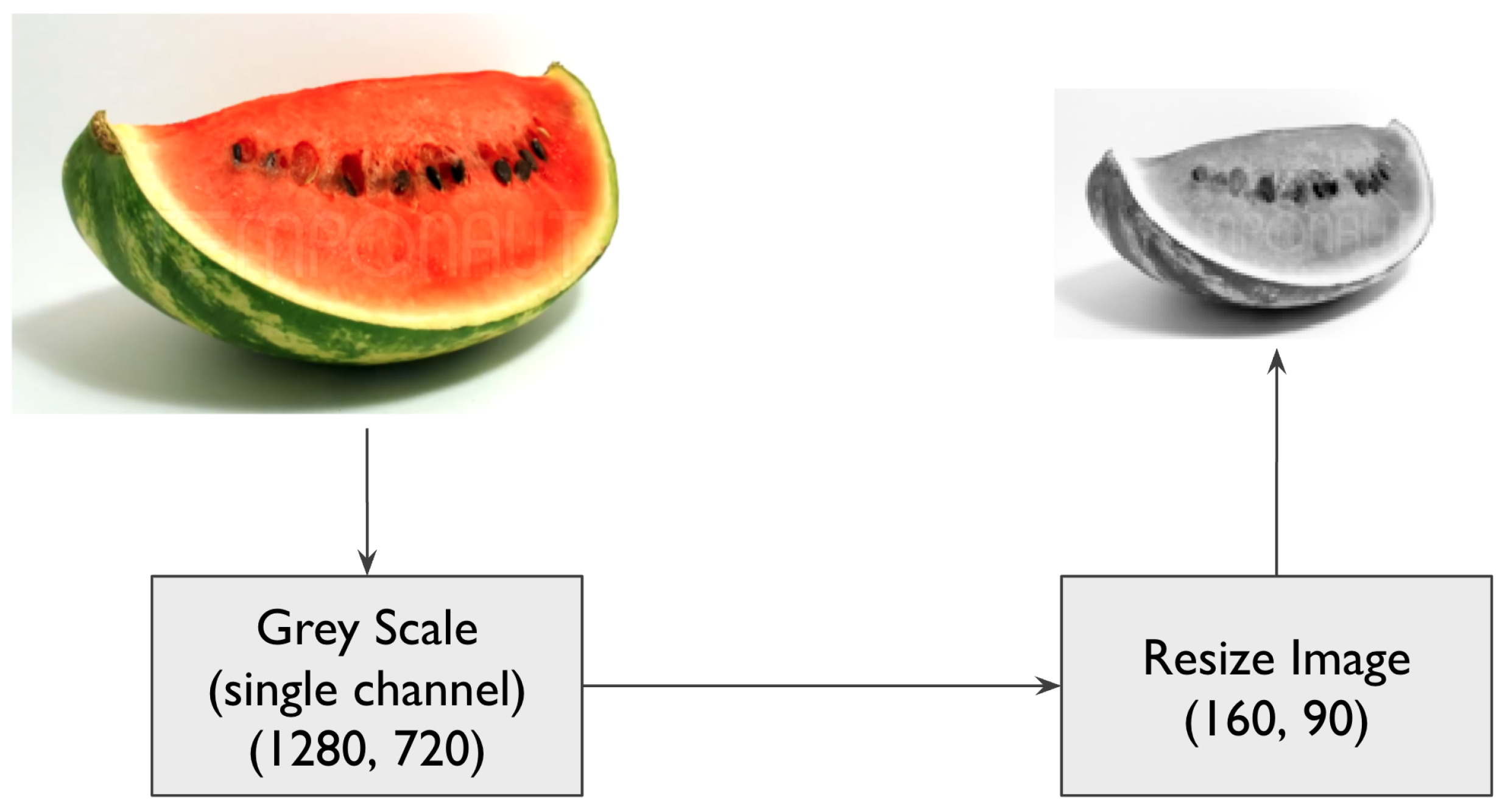
The experiment data was simplified to evaluate the most fundamental non-trivial version of the problem. Images were converted to a single grayscale channel and resized to 160 by 90 pixels. A diagram showing the two processing steps is shown in Figure 3.

3.1.2. Autoencoder Training and Validation

Autoencoders are a type of neural network architecture designed to learn efficient representations of input data in an unsupervised manner. They consist of two main components: an encoder and a decoder.

The encoder takes an input image and maps it to a lower-dimensional latent vector, effectively compressing the information into a more compact form. This latent vector is intended to capture the essential features and variations present in the input data. The decoder then takes this latent vector as input and attempts to reconstruct the original image.

In Figure 4, we show the autoencoder architecture used. Note that both the encoder and decoder structures are built with a set of convolutional layers and a fully connected layer of perceptrons, used to map the images into a latent space with 1000 dimensions. All activation functions are ReLUs.

The autoencoder is trained by minimizing the reconstruction error between the input image and the output, forcing the latent vector to retain the information necessary for accurate reconstruction. In consequence, the latent space becomes a learned representation, where different regions correspond to different characteristics of the input data.

We trained our autoencoder with a random split of the original dataset, where we used 80% of the data for training, 10% for validation, and 10% for testing, resulting in an overall split of 203 elements in the training set, 25 in the validation set, and 26 in the test set.

Additionally, we configured the training experiments with batches of 10 images each and 70 training epochs. See Figure 5 for an example batch.

Inspired by the work of Johnson J. et al. [47], we decided to use the pretrained VGG network to compute the perceptual loss, using VGG16 as a static feature extractor to compare images based on high-level semantic features rather than direct pixel differences.

Let ${\varphi }_j\left(x\right)$ denote the feature map activation from the j-th layer of the VGG16 network for an input image x. The perceptual loss, ${\mathcal{L}}_{perceptual}$, between a target image $x_a$ and a reconstructed image $x_b$ is defined as the sum of the squared Euclidean distances (L2 norm) between their feature maps at a set of pre-selected layers, J:

$${\mathcal{L}}_{perceptual}(x_a,x_b)=\sum _{j\in J}{\parallel {\varphi }_j\left(x_a\right)-{\varphi }_j\left(x_b\right)\parallel }_2^2$$

(2)

Furthermore, we explored a pixel-wise hybrid loss function, ${\mathcal{L}}_h$, which integrates a pixel-level constraint by adding a Mean Squared Error (MSE) term:

$${\mathcal{L}}_h(x_a,x_b)={\mathcal{L}}_{perceptual}(x_a,x_b)+\mathrm{MSE}(x_a,x_b)$$

(3)

In this case, the set of layers J was constructed from four VGG16 blocks:

• Block 1: Layers 0–3;
• Block 2: Layers 4–8;
• Block 3: Layers 9–15;
• Block 4: Layers 16–22.

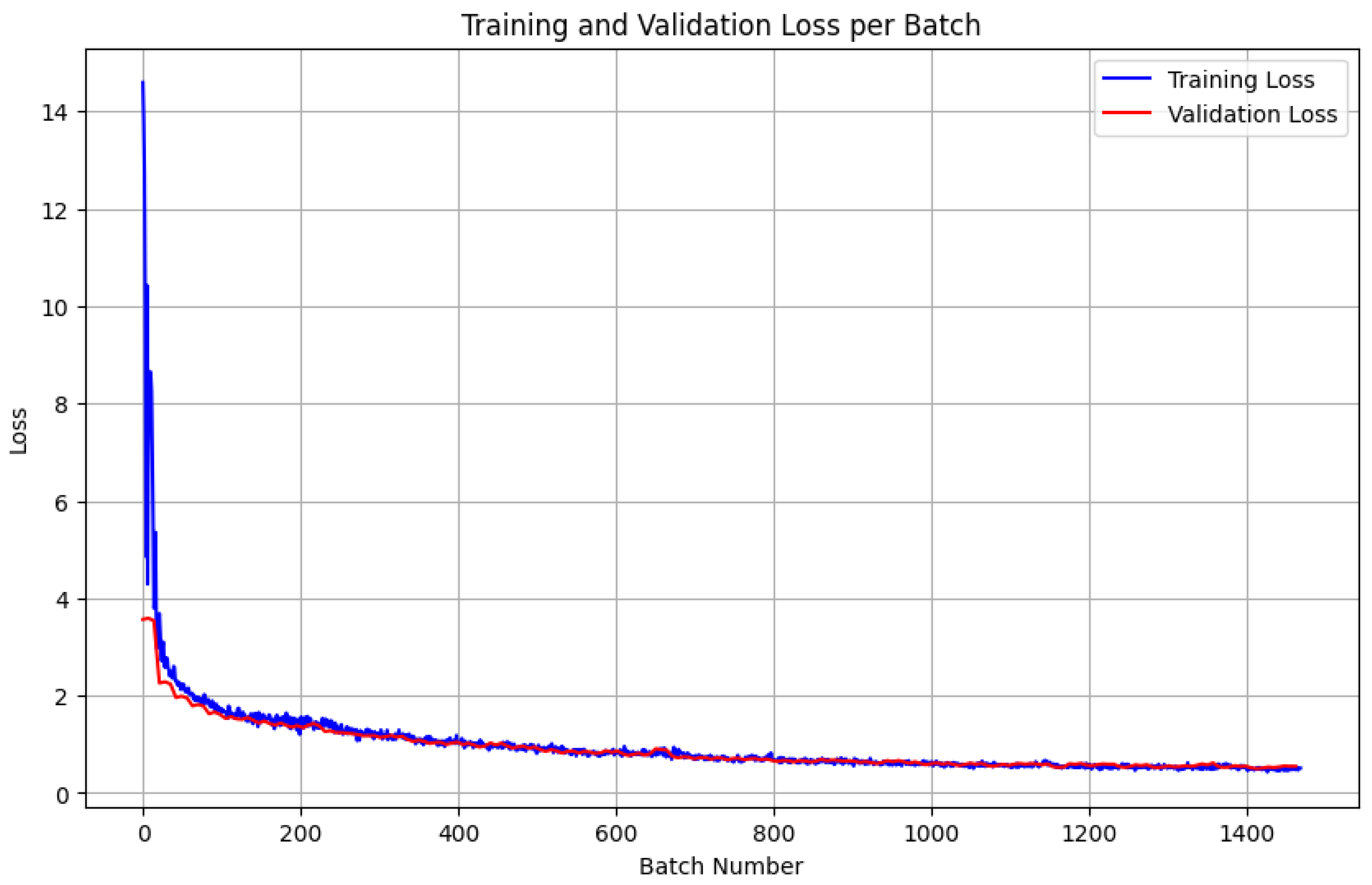
We selected the model trained with the sum of perceptual loss and MSE, as qualitatively we observed a better reconstruction of the correct gray shading and overall detail. Figure 6 shows some reconstruction examples taken during training, and in Figure 7 we present a plot of the training and validation loss. Finally, in Figure 8 we show the reconstruction results of the fully trained model.

3.1.3. Steering Vector Learning

We use the image labels in the dataset as the single attribute to edit, in which case, there should exist a steering vector to move from an image labeled as good to its corresponding state as rotten. Figure 9 shows a simplification of the steering vector’s effect. Note that we decided to relabel the images tagged as mild to good in order to frame the attribute editing process as a binary characteristic.

Figure 10 illustrates the learning process for this case study, in which we use the previously presented encoder m to transform image $I_1$ and image $I_0$ into their latent representations ${\omega }_1$ and ${\omega }_0$. Note that the rotten attribute a is present in $I_1$ but not in $I_0$, noted by $a=1$ for a rotten image and $a=0$ for a non-rotten or fresh image. The embedding ${\omega }_1$ is reconstructed using decoder g in image x, while ${\omega }_0$ is modified by adding vector E to it, resulting in a new latent projection $\overline{{\omega }_0}$ that, when decoded with g, results in the intervened version of the input image, $\overline{x}$. After obtaining the pair $(x,\overline{x})$, we can calculate a perceptual similarity error and use it as a loss metric. It is important to mention that, during the optimization of E, both $I_1$ and $I_0$ are not single images but batches of image pairs with the rotten binary attribute. We use the pretrained VGG16-based perceptual loss in Equation (2) as the loss function. Finally, we iteratively optimize vector E using an Adam optimizer with a learning rate of $5\times {10}^{-3}$ until it effectively minimizes the similarity error between the pair $(x,\overline{x})$.

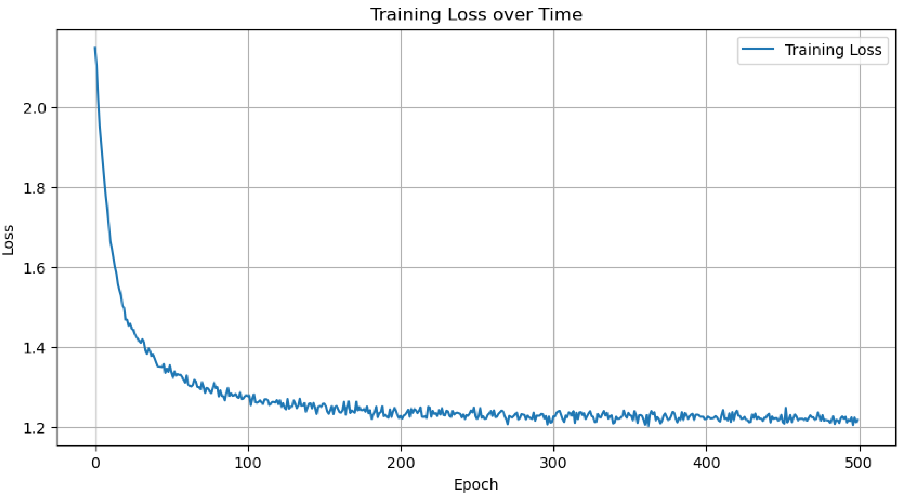
Figure 11 shows the training loss for the 500 epochs configured in the training sequence for the steering vector going from good to rotten, while Figure 12 shows the training experiment of the opposite steering vector, going from rotten to good.

Figure 13 and Figure 14 show the effects of applying a steering vector to image reconstructions. The “good-to-rotten” training was less stable and resulted in a higher final loss, despite significantly more training epochs (Figure 11), indicating that a lower learning rate could be beneficial. In the “good-to-rotten” transformation (Figure 13), the steered reconstruction exhibits artifacts associated with the target “rotten” label, such as molding, volume reduction, and overall darker tones. In the “rotten-to-good” transformation (Figure 14), these artifacts are reduced, but an entangled attribute emerges as a darkening of the background. To mitigate this, we hypothesize that replacing the standard perceptual loss (Equation (2)) with a hybrid loss function that adds a pixel-wise MSE component (Equation (3)) could further improve the disentanglement of this specific darkening.

We decided to repeat the training loop with slight random seed variations in order to test how reliable this training process is and to intuitively explore if there exists convergence between the experiment results. By repeating the training experiment, we expect to find steering vectors that converge in the solution space. To this end, we repeated the training sequence for both steering vectors 50 times each. We then used t-SNE to visualize the resulting vector sets in a lower-dimensional projection. Figure 15 and Figure 16 show the t-SNE projections of the good-to-rotten and rotten-to-good steering vectors, respectively. We use the default configuration of the TSNE implementation from the sklearn library [48], where perplexity is set to $30.0$, the maximum iteration parameter is set to 1000, and the learning rate is set to “auto” and calculated according to its documentation using the sample size and early exaggeration, which is automatically calculated.

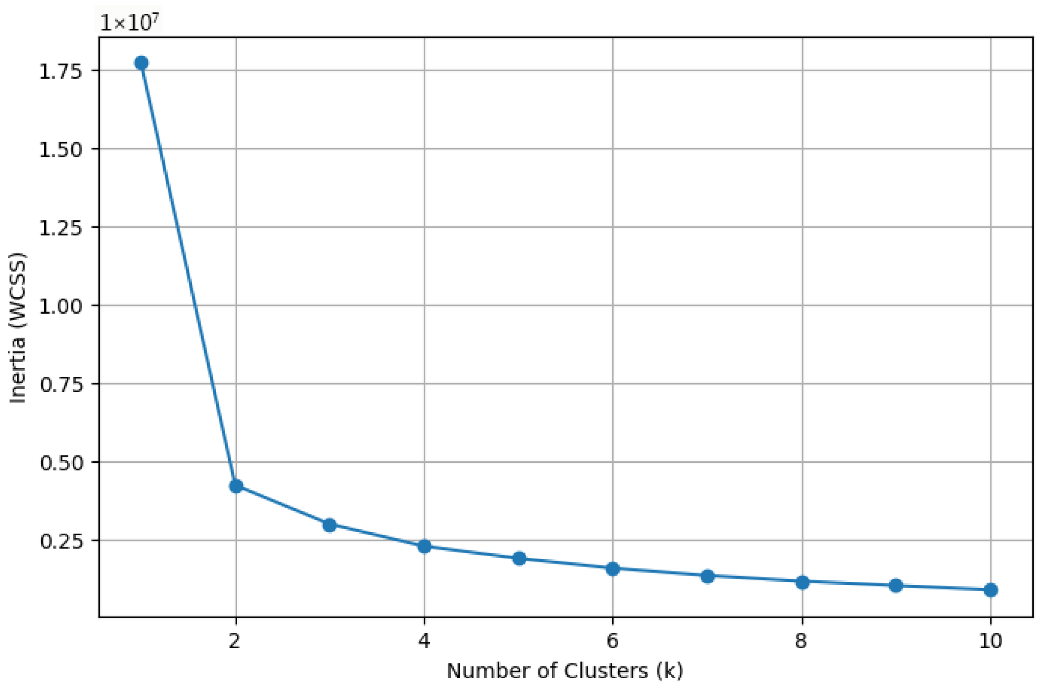
The color of elements in the plot comes from using the resulting t-SNE vector sets to fit a k-means clustering algorithm, finding clusters of similar vectors, with the expectation of finding convergence between the results. Intuitively we propose that there should exist one steering vector in the search space that achieves effective attribute manipulations. We show the corresponding k-means inertia plots in Figure 17 and Figure 18.

3.1.4. Interpretability Through Steering Vectors

We have shown how, using steering vectors, one can effectively manipulate the target attribute and how they converge to similar solutions across multiple experiments. In this section, we will explore how we can refine these vectors and progressively select relevant dimensions that achieve the target transformation, disentangling the space and providing an interpretable visualization.

We first perform statistical filtering to calculate a single representative vector of all 50 experimental observations. The core idea is to identify if each dimension is statistically different from 0, since this would mean that that particular vector feature is not relevant for the target transformation because it does not modify the latent projection. To perform this test, we use a one-sample t-test, where the null hypothesis H0 is that the mean value of the vector dimension tested is 0 and the alternative hypothesis H1 is that the mean is not 0. A one-sample t-test is appropriate for this type of filtering because, for each vector dimension tested, we have a single sample of 50 observations. We are not comparing two different sample groups; the test compares one group of observations to a fixed known number. Additionally, the standard deviation of the underlying population is not known; the t-test uses the t-distribution and is designed for these cases. The t-test assumes normality, as long as the sample size is large enough; even if the original population is not normally distributed, the distribution of the sample means will be approximately normal.

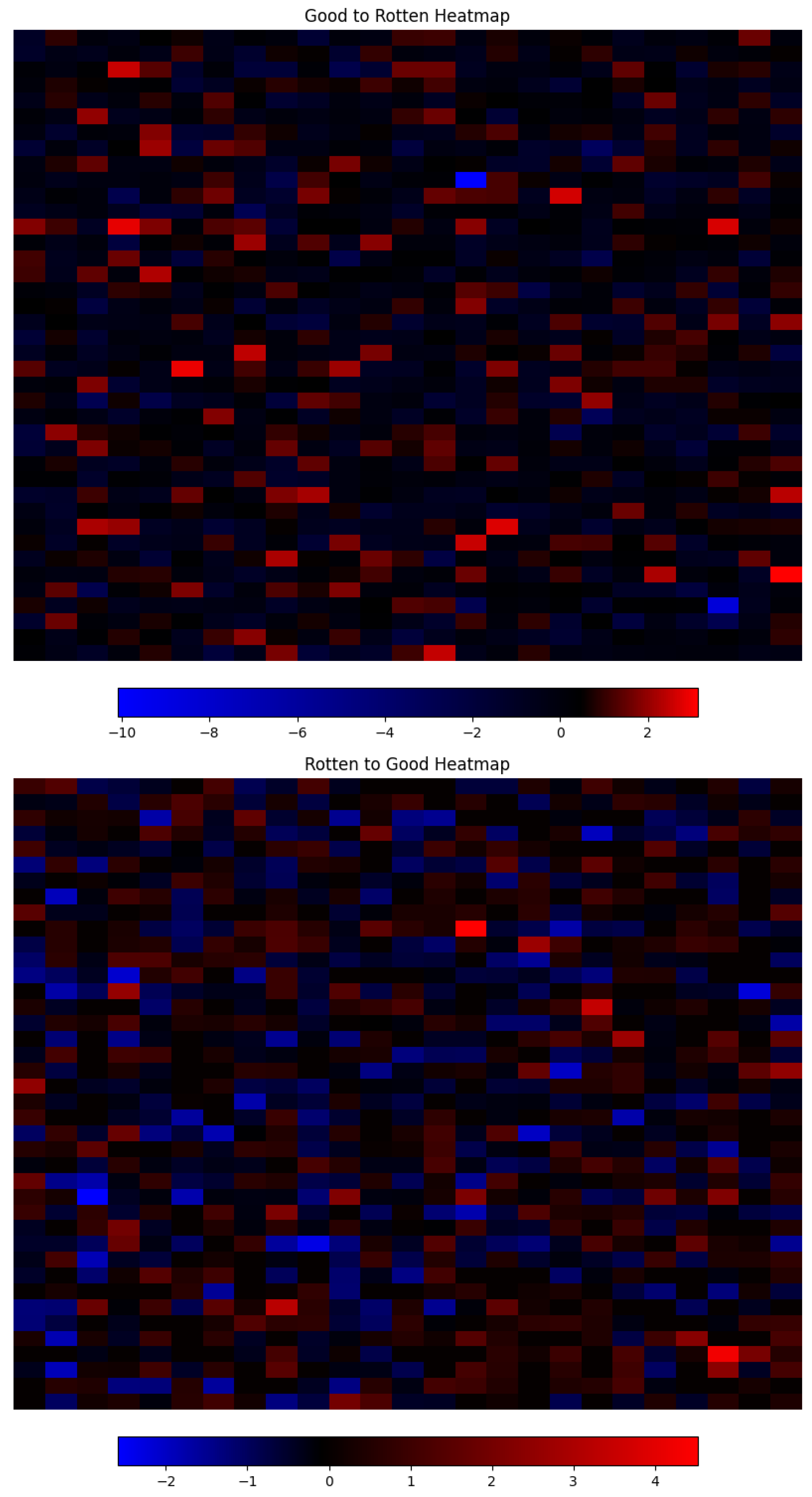
To build the representative vector, if the null hypothesis is accepted, we set the corresponding vector element to 0; if it is rejected, the observed mean is set. We use the scipy [49] python package implementation of the one-sample t-test to automate the testing process. Figure 19 shows a heatmap visualization of the resulting vectors.

Next we apply a directional filter, where we compare both vectors, good-to-rotten and rotten-to-good, element by element; if the values are of equal sign, then the feature is set to 0; otherwise, their respective values are maintained. This filter assumes that the learning process will find opposite vector elements for opposite attribute transformations and that the magnitude difference is only relevant if the directions are, in fact, opposite. It is important to note that it could be the case that for some attribute manipulations, the rate at which a certain dimension grows, represented by the magnitude of equal-signed vector values, relates to a relevant lesser characteristic, for example, the color intensity of a shadow. For now, this is beyond the scope of this exploration. 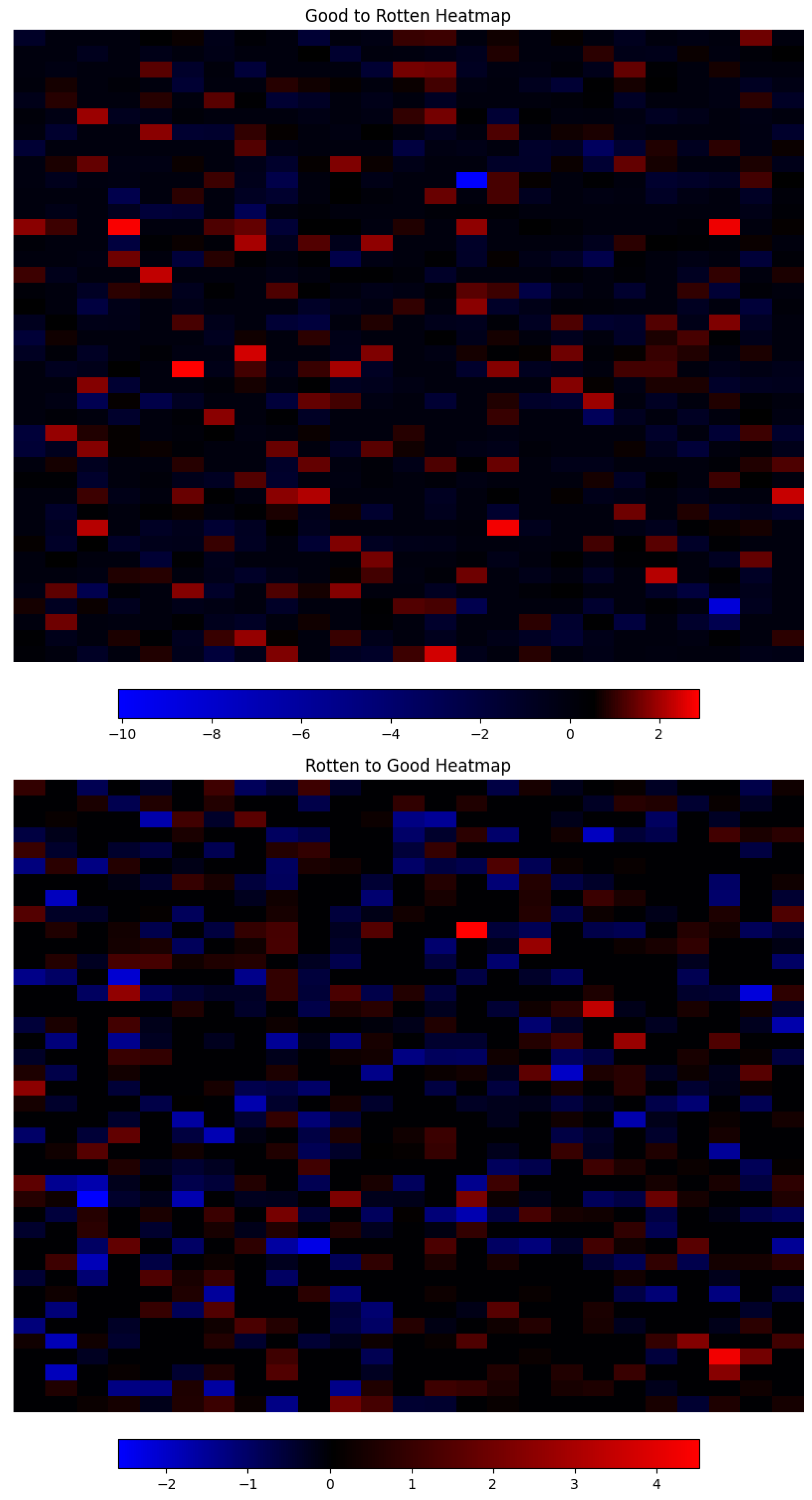Figure 20 shows the resulting vectors; it is observed that the overall number of features set to 0 increased when compared to the previous statistical filter.

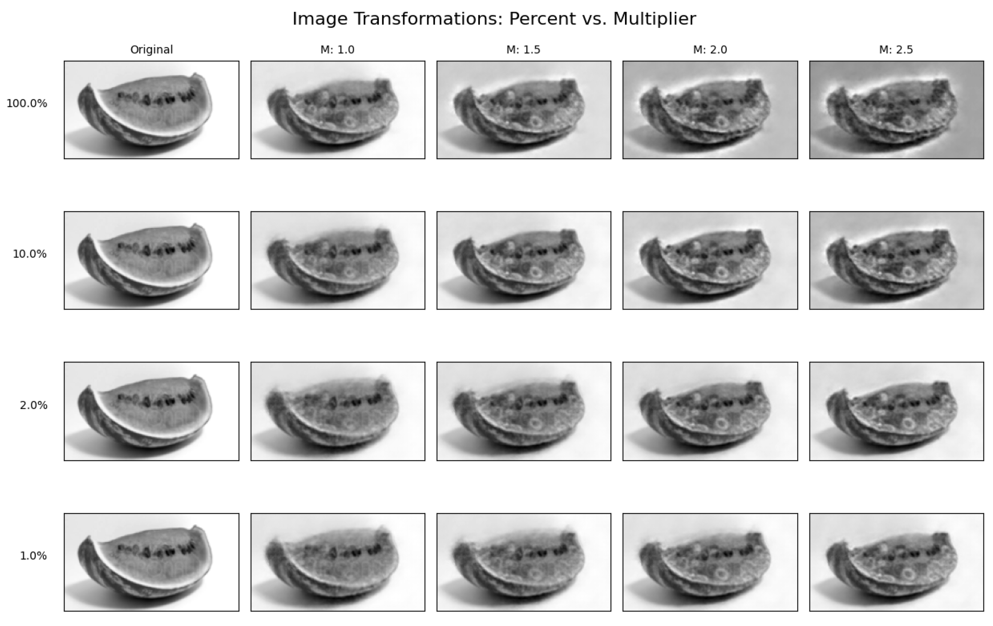
Using these refined vectors, we set up a new series of experiments. We test the effects of two types of manipulations, a saliency-based filter and a scalar multiplier. In this case, the saliency filter selects the feature dimensions whose vector element is within the largest specified percentage threshold, setting the vector value to 0 if it is not selected. This means that only the largest $x\%$ dimensions remain. For example, selecting 100% will leave all feature dimensions, while in this case, selecting 10% would leave the 100 most salient dimensions.

The scalar multiplier is a factor that is multiplied to all elements of the filtered sparse vector, scaling the effect of the non-zero dimensions. In

Table 1. good-to-rotten experimental values for magnitude filter and scalar multiplier.

Good to Rotten
	Symbol	Values
Magnitude filter percentage	x	[100.0, 10.0, 2.0, 1.0]
Multiplier	m	[1.0, 1.5, 2.0, 2.5]

and

Table 2. rotten-to-good experimental values for magnitude filter and scalar multiplier.

Rotten to Good
	Symbol	Values
Magnitude filter percentage	x	[100.0, 10.0, 2.0, 1.0]
Multiplier	m	[1.0, 1.5, 2.0, 2.5]

, we list the discrete values of multiplier m and magnitude filter x used in the experiment. We explore the effect of these combinations using a grid, where we reconstruct the input image after each modified perturbation is added to its latent projection; we show this grid in Figure 21 and Figure 22.

In Figure 22, we show the reconstruction grid of good-to-rotten images. Note how by using the values $x=2\%$ and $m=2.0$ the decoder is able to reconstruct an image $I_{2,2}$ that is qualitatively close to the original reconstruction, which used all 1000 dimensions. Image $I_{2,2}$ exhibits a less blurry reconstruction, little to no effect on background shades, and the presence of mold in the right places. 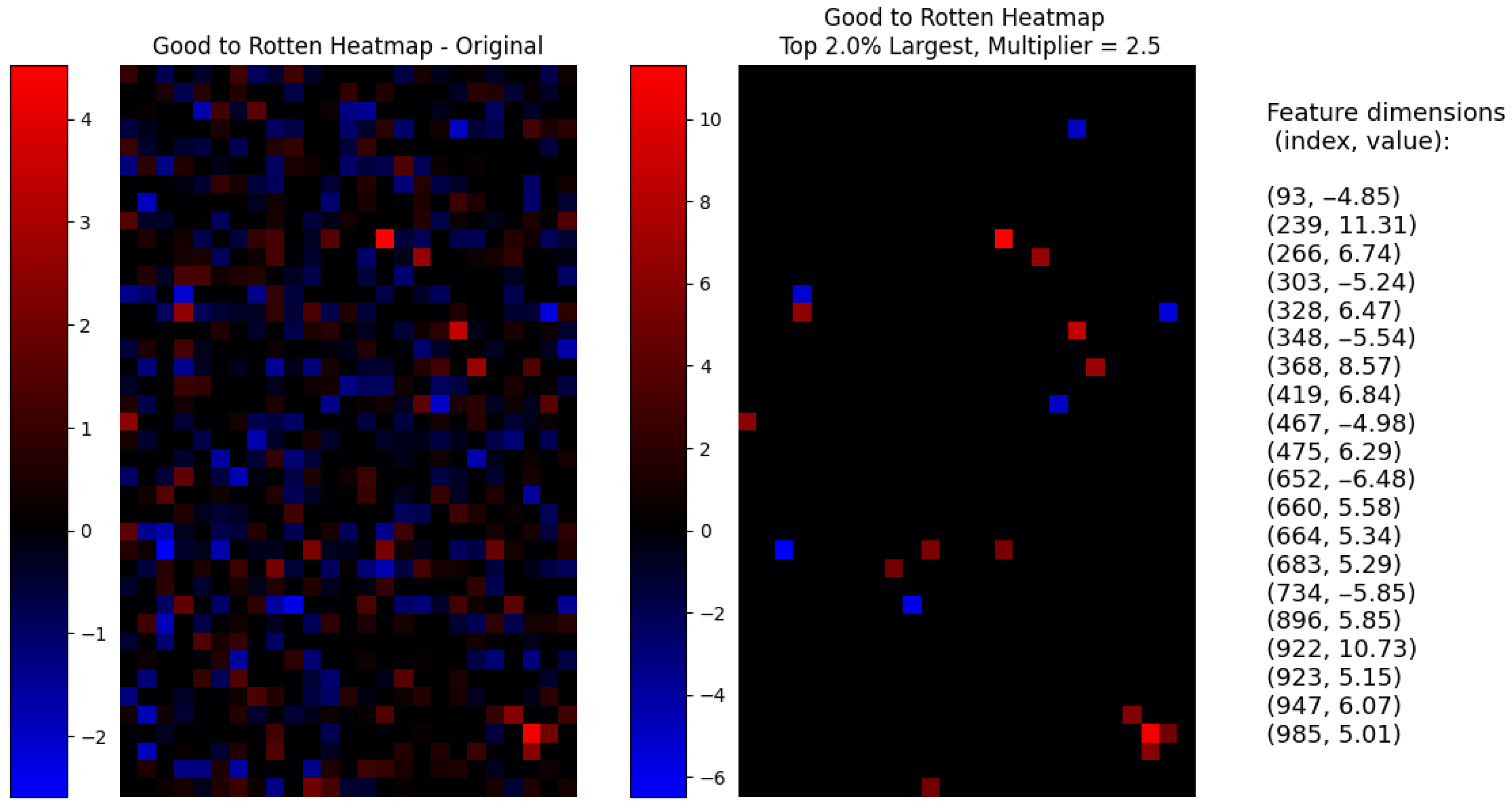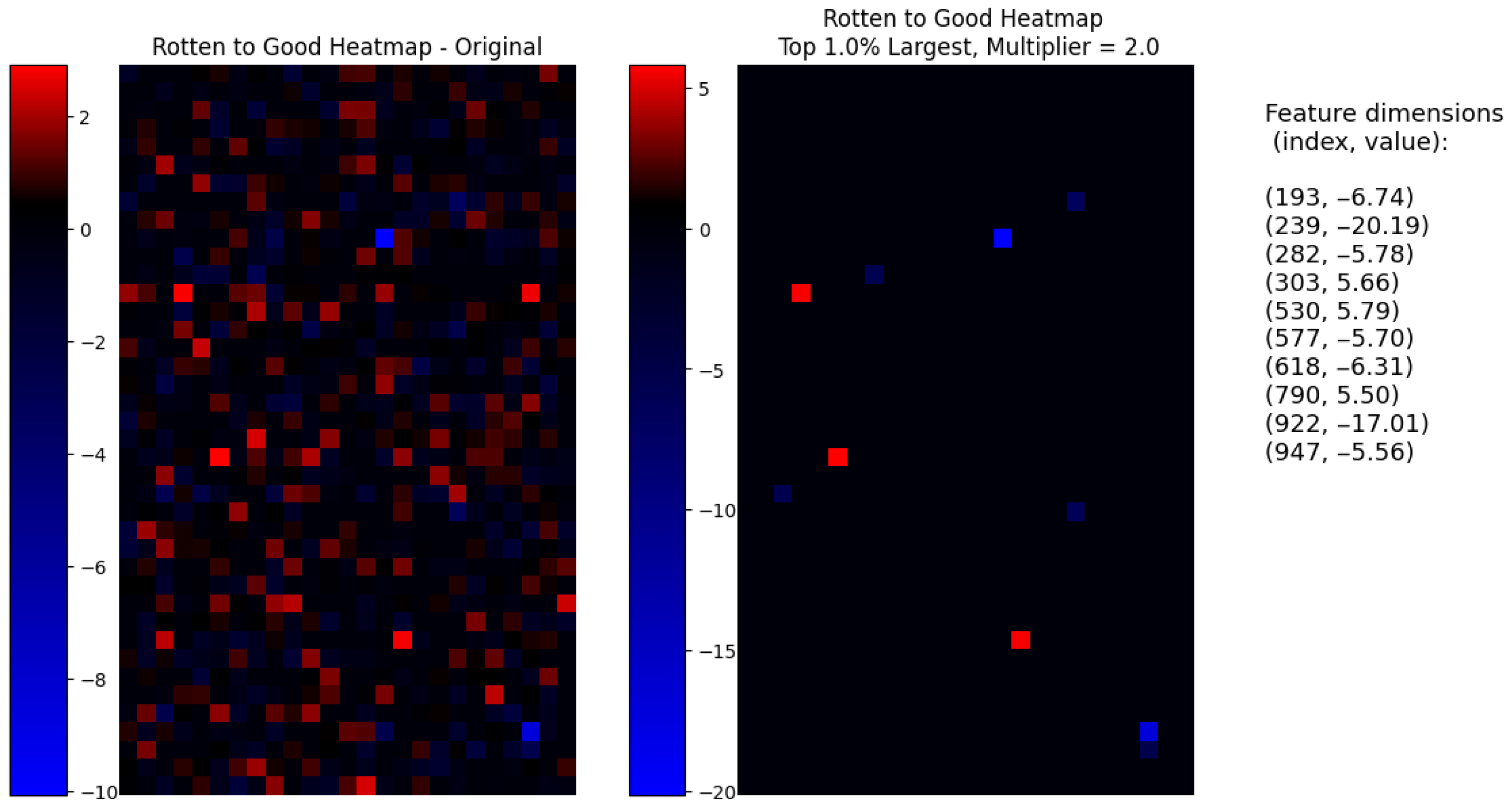This means that by selecting only $2\%$ or only 20 dimensions out of 1000 and multiplying the corresponding steering vector elements by $m=2$, the model is able to generate effective attribute-manipulated images, showing how the rotten attribute on a healthy image depends on these 20 dimensions. In the heatmap shown in Figure 23, we present an interpretable visualization of the resulting selection, along with a list of the dimension indices and their corresponding steering vector magnitudes.

A similar result is shown in the opposite transformation in Figure 22, going from the rotten to the good attribute. In this case, by selecting $x=1\%$ and $m=2.0$, only 10 out of 1000 dimensions, we achieve an even better reconstruction than the original parameters achieved. It can be observed how the volume of the subject is better integrated into the rest of the image, and there are fewer coloration artifacts where mold marks used to be and the reconstruction is less blurry. There is, however, a negative effect on the background color, which is noticeably darker. If we inspect the rest of the images, we can see how the background becomes darker as the multiplier and dimensions grow, suggesting that this is, in fact, an entangled attribute that was not fully disentangled during the learning process. In Figure 24, we visualize the corresponding interpretable selection heatmap along with the dimension–value pairs of the steering vector elements that achieved this manipulation.

Finally, we identified that there is an overlap in the selected dimensions for the opposite transformations; the dimensions in

Table 3. Overlapping dimensions for both transformation directions.

Dimension Index	Good-to-Rotten Value	Rotten-to-Good Value
239	11.31	−20.19
303	−5.24	5.66
922	10.73	−17.01
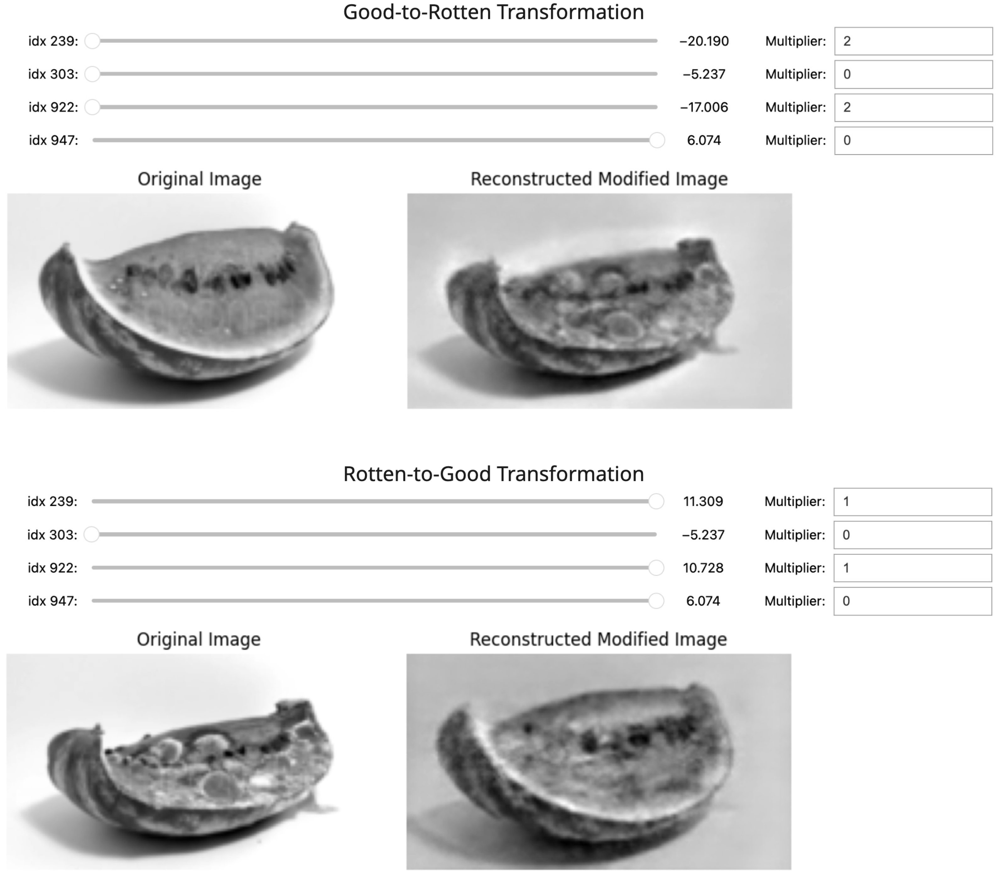
947	6.07	−5.56

appear on both filtered steering vectors with opposite directions based on their sign. Following this selection, we explored the effect of introducing manipulations only on these four feature dimensions and qualitatively evaluating their effect on the target attribute in the reconstructed image. From these experiments, we further identified that by manipulating dimensions 239 and 922 in opposite directions, one can effectively transform the target attribute. We show this effect in Figure 25, where we disable dimensions 303 and 947 by multiplying them by 0. In the same figure, we include the sliders used in the experimentation to modify the value of the steering vector in its respective dimension. The maximum and minimum values of each slider correspond to the values identified in each direction of the refined steering vectors shown in Table 3. In the rotten-to-good transformation, selecting dimensions 303 and 947 and using the original positive steering values are sufficient to achieve an effective manipulation, while in the good-to-rotten transformation, we need to multiply the selected dimensions by a factor of 2 and slide them to negative values.

3.1.5. Model Explainability

In this section, we will answer the initially selected explainability questions M3 and P6 from Section 2.2.

Question M3 states: “What are the consequences of making a different decision or adjusting a parameter?” We have shown how, by adjusting the magnitude and sign of a select few feature dimensions in the latent projection, the model is able to reconstruct images with an altered attribute. The consequence of adjusting them produces an identifiable effect on the model output, and thus we are now able to interpret what a certain adjustment in a parameter will produce in regard to the target attribute. So we can answer this question: by modifying dimensions 239 and 922, one can effectively say that the consequence will be a manipulation of the rotten attribute. Furthermore, we have identified not only which dimensions need to change but also which ones need to remain undisturbed to achieve the desired result, advancing the goal of unifying feature attributions and explanations.

Question P6 states: “Is there anything that can be done to have a different outcome?” We have in fact identified which manipulations should be carried out to produce opposite image attributes. By adding the identified element values to their respective features and by adjusting their magnitude, we have shown multiple different outcomes with varying effects. And so, a different outcome is achievable through these controlled manipulations.

4. Discussion

In this section we interpret the previous results, discuss advantages, and limitations of our proposal.

The main results are the visualizations in Figure 23 and Figure 24, where we show how, after the refinement process, we’re able to identify a minimal set of dimensions, their magnitude and sign to achieve effective control of the target attribute. This visualization enables interpretations of the generative mechanism of the model. This level of interpretability is a crucial advantage as it not only displays which latent dimensions should be modified, the rate of these modifications, but also makes it clear which ones should remain unchanged. This is an indirect separation of content and style dimensions, a central concept in latent space disentanglement [5,7].

The next noteworthy results are the dimension overlaps in Table 3 and their exploration in Figure 25, where we show how, by manipulating only 2 feature dimensions, the model is able to produce modified reconstructions that control the target attribute. This result showcases the effectiveness of the steering vectors learned as disentanglement tools for pretrained generative models, presenting an advantage over models that require conditional training or other trained proxy models [11,12].

One secondary result that is important to highlight is the presence of two clusters found in the clustering exploration shown in Figure 15 and Figure 17. This suggests that there were two equally valid solutions for the correspondent steering vector. The proposed methodology, as explained in the previous Section 3, is at its core an optimization problem to minimize the selected loss function. This means that the selected loss function could in fact have several local minima and the observed outlier solution is most likely found in one of them. This implies that the method will find effective steering vectors but depends on the optimization method to navigate the loss function topology. The refinement process with statistical tests is a robust way to protect the method against these types of outlier solutions that, while valid in terms of the targeted loss, might not be the the global minimum since experiments initialized with different random states, or a different optimizer, do not converge to it. This highlights the importance of repeating the vector training experiment enough times to gather a sufficient number of observations.

Regarding the limitations of our method, we identified the first one from its applicability. As we mentioned in the taxonomy presented in Section 2.2, this method is Model-specific in the sense that it would not be applicable to denoising-type vision generative models, as these models rely on integrating noise on the latent projection and learning effective sequential transformations to remove it [50]. This means that in order to utilize the presented contrast technique to learn steering vectors, we would need to modify the framework to train multiple steering vectors between denoising steps or change the mask-like addition of the vector and append it instead to the latent projection vector, an approach similar to how diffusion models aggregate multimodal inputs [50]. This current limitation requires further research.

Another important limitation is the fact that this method is not generalizable to fully explain multiclass attributes. For example, the mild status is not a target of the steering vector learned during the contrast learning sequence. This is because only binary attributes provide the complete absence or presence of a certain characteristic, which is necessary to learn the proposed steering vector. Multiclass states could or could not appear during the incremental application of the steering vector, but classification of these types of state requires an external attribute classifier that is beyond the scope of this work.

The specific framework to utilize this method as a potential attacking technique is not explored in this paper, but it does remain a concern and limitation worth noting. The method itself could be used as a form of extraction attack, used to infer parameters of the generative model or the mapping function. By observing how multiple feature maps manipulate image attributes, an attacker might be able to reconstruct model weights or train a proxy model that emulates the behavior of the original. This form of attack would need to be performed with access to the latent space embedding, which can be protected as a countermeasure.

By mapping features in the latent space to specific image attributes, the method could reveal correlations between seemingly unrelated attributes, which are entangled feature vectors present in the training data; this could expose sensitive attributes of the observations used to train the original generative model. This is the same capability that a developer would use to identify training biases. If the generative model was trained on a dataset containing images with protected attributes (like age or gender), manipulating certain features might reveal information about these protected attributes. Like a training bias that correlates attributes with certain racial groups, age groups, or other sensitive categories. It may also be possible to infer whether specific observations were part of the original generative model training dataset. Suppose we introduce a known image to be edited by applying the steering vector in its latent projection; analyzing how effective the feature map is at modifying the output could reveal whether these specific observations were used during the training phase of the generative model, which is another ethic and privacy limitation of our solution.

5. Conclusions and Future Work

We have shown how our proposed method effectively learns steering vectors that can manipulate a target attribute without using pretrained classifiers. We showcased how the contrastive learning setup is effective at avoiding the effect of classification errors and how it can be utilized to disentangle a target attribute from a pretrained autoencoder. This is especially relevant since it avoids the need for conditional training and broadens its applicability. We explored an intuitive approach to show the convergence of trained steering vectors towards a single solution, but further formal exploration of this characteristic will be explored in future work. We contribute an innovative approach in the controllable generation domain that eliminates the need for a conditional training setup through a contrastive learning setup, enabling its use with pretrained generative models.

We also showcased how the learned vectors can be filtered and refined to serve as interpretations of the generative mechanism of a model and can offer a way to simplify the solution space to achieve attribute explanations. This method reduced the total set of intervened dimensions to only $2\%$ and $1\%$ of the initial 1000 dimensions in each case and then further reduced the selection to only 2 dimensions, first by exploring the intersection of the rotten-to-good and good-to-rotten sets and then qualitatively evaluating the transformation effects of modifications in the intersection. We were able to identify the magnitude and direction of the manipulation necessary to achieve attribute control, relating these findings to interpretable visualizations and, in the second step, to human-readable explainability questions. We contribute an XAI method that uses steering vectors as knowledge to interpret the generative mechanism of the model. Additionally, we provide a first step toward unifying feature attributions and explanations, highlighting dimensions that require modifications and those that should stay unchanged to produce a target outcome. This capacity for precise, minimal intervention positions our work as a powerful tool to empower causal discovery. While LIME and SHAP reveal correlations between inputs and outputs, our method provides a more structured, causal lever. By identifying the minimal set of dimensions required to enact a change while leaving others untouched, our technique facilitates controlled experiments within the latent space. This is a crucial step towards understanding the causal relationships the model has learned. Rather than relying on random perturbations, our steering vectors enable informed, directional interventions that drastically reduce the variable space, as shown by our ability to shrink a 1000-dimensional problem. This presents a significant opportunity to overcome the scalability barriers of current causal discovery techniques, using the generative model itself to uncover the functional relationships it has encoded. In fact, this is the most important future research direction that we will pursue, extending this method to Causal Explanations

The next promising future research avenue is the introduction of different optimization algorithms to improve dimension filtering. This would require an objective function that could be based on the same contrastive similarity function presented but could also be based on a pretrained classification method that is more suitable for few-shot applications or a fine-tuned vision model to help mitigate the compound error effect. Additionally, we will work on further testing the steering vector learning process so as to mitigate the effect of entangled background attributes in the case study presented. We will also explore the modification of the proposed perceptual loss to the hybrid pixel-wise version and other hyperparameter combinations in various applications.

We also aim to increase the complexity of the problem to test the method on multiple-channel images, a more diverse set of subject types that exhibit variations in the target attribute, and other types of vision generative models. This will necessarily need to be supported by quantitative metrics, especially if we aim to benchmark the proposed control method against conditional training approaches, perhaps using attribute classification accuracy.

Lastly, regarding the applicability of the technique, there is an opportunity to adapt the contrastive learning setup to diffusion-based models by adapting it to a step-by-step denoising pattern to achieve effective manipulations and to utilize the mask-like addition of the steering vector to achieve latent dimension explanations. This potential application would require significant research to adapt the method in its current state.

Our work builds a link between controllability and explainability. By showing that steering vectors can be learned without attribute classifiers and subsequently refined into concise interpretations, we provide a unified framework that not only directs a model’s output but interprets its internal logic, going beyond simple manipulations. Our method offers a scalable pathway to transform the opaque latent space of pretrained generative models into a structured and understandable system. We believe that our work advances our ability to direct, comprehend, and ultimately trust the creative mechanisms of generative models.