Comprehensive Assessment of Wind Energy Potential with a Hybrid GRU–Weibull Prediction Model

Abstract

Wind energy is a critical renewable resource in the global effort toward sustainable development and climate change mitigation. This paper introduces a hybrid forecasting framework that integrates multistep gated recurrent unit (GRU) modeling with Weibull distribution analysis to assess wind energy potential and predict long-term wind speed dynamics. The approach combines deterministic and probabilistic components, improving robustness against seasonal variability and uncertainties. To demonstrate its effectiveness, the framework was applied to hourly wind data collected from multiple stations across diverse geographical regions in Turkey. Weibull parameters, wind power density, capacity factor, and annual energy production were estimated, while five machine learning models were compared for forecasting accuracy. The GRU model outperformed alternative methods, and the hybrid GRU–Weibull approach produced highly consistent forecasts aligned with historical patterns. Results highlight that the proposed framework offers a reliable and transferable methodology for evaluating wind energy resources, with applicability beyond the case study region.

1. Introduction

Global energy consumption is steadily increasing in tandem with population growth, urbanization, and rapid technological advancements. This trend has prompted nations to seek sustainable energy solutions that aim to mitigate environmental impacts and minimize dependence on fossil fuels [1]. Within this context, renewable energy sources have gained increasing prominence worldwide and have become central to energy policies. Wind energy stands out as a renewable and environmentally friendly resource [2]. Considering the environmental damage and limited reserves associated with fossil fuels, wind energy offers a sustainable alternative for the production of clean energy. It contributes to combating climate change by reducing carbon emissions, minimizes air pollution, and promotes the utilization of local resources, thereby decreasing foreign dependency. Additionally, it supports economic development. Advancements in technology have made wind turbines more efficient and cost-effective, making them a viable solution for both small-scale and large-scale energy needs [3,4].

The widespread adoption of wind energy is regarded as one of the foundational pillars of future clean and sustainable energy policies. According to the 2025 Global Wind Report [5], based on data from all regions of the world, global wind energy capacity grew significantly in 2024. With 109 GW of onshore wind and 8 GW of offshore wind installations, the global cumulative wind energy capacity reached 1136 GW. This capacity is distributed across all continents, and a total of 55 countries installed wind turbines throughout 2024. In terms of new installations, China led the world in added wind energy capacity in 2024, followed by the United States, Germany, India, and Brazil. These same countries occupied the top five positions in terms of total installed wind energy capacity at the end of 2024. The report forecasts a compound annual growth rate of 8.8% for the wind sector, implying the addition of 981 GW of wind energy capacity worldwide by 2030. Turkey’s wind energy potential is estimated at 48 GW onshore and 32 GW offshore, with the total installed capacity reaching 13.8 GW by the end of 2024. In the same year, 1.3 GW of new installations increased wind power’s contribution to 11.3% of national electricity production, underscoring the sector’s strong growth trajectory.

Accurate estimation of wind energy potential requires statistical modeling of wind speed. The Weibull distribution is one of the most effective models for representing the probability density of wind speed data. The two-parameter Weibull model provides a high-accuracy representation of wind speed frequency distributions [6]. Numerous researchers have conducted studies on various methods for determining the parameters of this distribution to enable precise calculation of wind energy potential. Rüstemli et al. [7] applied the two-parameter Weibull distribution with the maximum likelihood estimation method to assess wind energy potential, and their GIS-based analysis identified the study area as favorable for wind power development. Nymphas and Teliat [6] utilized five numerical methods—Weibull-two (W), Mixture Weibull (MW), Gamma (G), lognormal (LN), and normal (N) distributions—to estimate Weibull parameters for wind speed characterization in assessing Nigeria’s wind energy potential. The methods’ effectiveness was evaluated using Kolmogorov–Smirnov (K-S) maximum error, root mean square error ($RMSE$), and chi-square ($X^2$) goodness-of-fit tests. The MW method was concluded to be the most suitable for accurately estimating Nigeria’s wind energy potential. El Kihel et al. [8] assessed the wind energy potential in five different regions of Taza Province, Morocco. A comprehensive statistical analysis was conducted using the MLE, Jestus method, Lysen method, Moroccan method, and graphical method (GM). According to the results, Region 3 (Taza) emerged as the area with the highest wind energy potential, exhibiting a capacity factor ($CF$) of 30.84% and an annual energy production ($AEP$) of 9.18 GWh/year. Yadav et al. [9] conducted a comparative analysis of various numerical methods to determine wind power potential in different regions of Andhra Pradesh, India. The methods included method of moments (MoM), energy pattern factor method (EPFM), maximum likelihood method (MLM), energy density method (EDM), energy pattern factor method of Sathyajith (EPFMS), Rayleigh distribution, and a novel method, novel energy pattern factor method (NEPFM). NEPFM yielded the most successful results for Visakhapatnam, Amaravati, and Tirupati, while MLM performed best for Rajamahendravaram. The Rayleigh distribution was identified as the most suitable model for cumulative density estimation, particularly in Visakhapatnam and Amaravati. Aziz et al. [10] compared 14 different methods for estimating Weibull distribution parameters (k, the Weibull shape parameter, and c, the Weibull scale parameter) using 10 years of hourly wind data from three distinct wind fields. The results indicated that the EPFM was the most suitable across all wind speeds. The wind variability method (WVM) and Moroccan method (MoroM) were deemed inadequate. Other methods generally provided acceptable results. Furthermore, as elevation increases, the k parameter decreases, while the c parameter increases. These findings highlight the importance of method selection for accurate wind energy potential estimation. Wadi and Elmasry [11] analyzed the wind energy potential in Istanbul’s Çatalca region using the two-parameter Weibull distribution. Weibull parameters were calculated via six methods (GM, MoM, EPFM, mean standard deviation, power density, and genetic algorithm) and compared using statistical metrics. The genetic algorithm provided the most accurate estimates, whereas the energy pattern factor method yielded the weakest results. Overall, all methods demonstrated acceptable performance levels. Although the Weibull distribution is effective for modeling historical data, machine learning (ML) techniques have become indispensable for future projections due to climate change and long-term trends. In wind energy production, particularly for short- and long-term forecasting, these methods are widely employed, providing insights from complex and variable meteorological data. Demolli et al. [12] performed long-term wind power forecasting based on daily wind speed data using five ML algorithms: least absolute shrinkage and selection operator (LASSO), k-nearest neighbors (kNN), extreme gradient boosting (XGBoost), random forest (RF), and support vector regression (SVR). The results demonstrated that ML algorithms can be utilized to predict long-term wind power values based on historical wind speed data. Alkesaiberi et al. [13] optimized the hyperparameters of Gaussian process regression (GPR), SVR, and ensemble learning models (boosted trees and bagged trees) using Bayesian optimization (BO) to forecast wind power. Dynamic information structures were incorporated to further enhance the predictive performance of the examined models. The results indicated that the optimized GPR and ensemble models outperformed other ML models. Zhang et al. [14] developed a hybrid model named EWP-CS-RELM to improve the accuracy of wind speed forecasting. The model employed a secondary decomposition method combining ensemble empirical mode decomposition (EEMD) and wavelet packet transform (WPT) to prevent pattern overlaps and reduce inter-component interactions. Tested on data from four seasons at two wind farms in Shandong, China, the model was compared against seven alternative methods and achieved the lowest statistical errors, yielding the most successful outcomes. Ti et al. [15] developed a novel ML-based wake model to enhance power forecasting performance in wind farms. The study revealed that the artificial neural network (ANN) model could predict wind power at a reasonable level, demonstrating superior performance compared to analytical models due to its flexibility in modeling nonlinear structures in the process. Mokarram and Pham [16] utilized advanced deep learning techniques and GIS to predict the energy output of wind turbines. The study focused on estimating the energy production of horizontal- and vertical-axis wind turbines using Markov and Cellular Automata–Markov (CA-Markov) models in conjunction with deep learning methods such as long short-term memory (LSTM), LSTM–wavelet, and SVR. The LSTM–wavelet hybrid model exhibited superior performance with an accuracy rate exceeding 90%, owing to its effective management of data instability and noise reduction. Bouabdallaoui et al. [17] explored the application of four artificial intelligence approaches—support vector machines (SVMs), decision trees, adaptive neuro-fuzzy inference systems (ANFIS), and ANNs—to forecast wind energy production at a wind farm in Yalova, Turkey. After comparison to actual values, SVM provided superior performance, while ANFIS proved less effective in this context. dos Santos et al. [18] analyzed hourly wind speed data from 575 meteorological stations in Brazil. A mixture of Weibull–Weibull distributions was applied to the measured wind speed series. The expectation–maximization (EM) algorithm was used to estimate the Weibull–Weibull distribution parameters. Based on results from each meteorological station and use of the inverse distance weighting (IDW) method, wind energy production was estimated for locations without wind speed data. The results indicated that the model successfully predicted wind energy density over large areas and is applicable in other countries. Malakouti [19] predicted power generation from a SCADA system using ML methods such as extra trees, light gradient boosting machine (LightGBM), gradient boosting regressor, decision tree, AdaBoost, and ridge. The extra trees algorithm demonstrated the best performance in accurately predicting turbine power output, while the ridge algorithm exhibited the lowest performance. Rutherford et al. [20] presented a novel ML-based method that transforms variations in a local numerical weather prediction (NWP) model’s wind speed output at 10 m height into ensemble-based energy forecasts at 100 m height. The developed method improved forecast accuracy by up to 9% compared to deterministic models and also provided valuable insights into forecast uncertainty.

Compared to ensemble methods such as RF, XGBoost, and gradient boosting, deep learning techniques have demonstrated enhanced capabilities to model complex temporal dependencies within time series data, particularly for applications such as wind speed prediction [21]. The recurrent architecture of the gated recurrent unit (GRU), an efficient extension of the recurrent neural network (RNN), excels in processing sequential information by addressing challenges such as long-term memory retention and computational efficiency through simplified gating structures [22]. In the context of wind forecasting, GRU models have shown superior performance in capturing dynamic patterns, such as diurnal variations and stochastic fluctuations, outperforming tree-based ensembles in metrics such as $RMSE$ for multistep predictions [23,24]. Given these strengths, integrating the GRU with the Weibull distribution in a hybrid framework offers a promising and underexplored strategy for the accurate assessment of wind energy resources. Recent advances in wind power forecasting have explored innovative approaches, including federated learning and recurrent neural networks (RNNs). For instance, federated learning techniques, as demonstrated in studies such as [25], enable decentralized training across multiple sites while preserving data privacy, offering scalability but at higher computational cost. Similarly, RNN-based methods, such as those employing LSTM or stacked LSTM architectures [26], have shown improved accuracy in offshore wind forecasting, particularly for short-term predictions. However, these approaches often rely on complex preprocessing or lack integrated probabilistic modeling for uncertainty management. The integration of machine learning with statistical models for wind forecasting has implemented in a diversity of approaches, including LSTM–Weibull and EEMD–GRU hybrids. LSTM–Weibull typically employs static Weibull parameter estimation, while EEMD–GRU relies on data decomposition techniques to enhance prediction accuracy. Our proposed GRU–Weibull framework introduces a novel approach by dynamically combining GRU’s time-series capabilities with Weibull modeling, aiming to address limitations in scalability and adaptability across multiple sites. This positions our method to potentially offer distinct advantages over existing hybrids, which will be explored in the context of Turkey’s diverse wind regimes. In time-series forecasting studies, hybrid GRU models formed by combining GRU with other architectures are frequently used to improve predictive accuracy and handle complex patterns. Gao et al. [27] proposed a hybrid GRU framework integrating CEEMDAN decomposition, convolutional layers, and attention mechanisms for improved prediction of energy consumption, demonstrating superior performance over traditional methods in real-world datasets.

Turkey’s geographical diversity, including its extensive coastlines, varied topography, and regions exposed to maritime influences, provides substantial wind energy potential. The Marmara and Aegean regions exhibit the highest theoretical capacity, supported by favorable wind regimes and developed infrastructure, while the Mediterranean region offers localized opportunities despite generally lower wind speeds. Central Anatolia is more limited due to its enclosed terrain, although certain areas remain suitable for investment. The Black Sea, Eastern Anatolia, and Southeastern Anatolia contribute less overall yet still present localized wind energy potential that can be harnessed under suitable conditions. This study aimed to contribute to the evidence-based elucidation of Turkey’s wind energy potential and to guide investment planning. Within the scope of this paper, the term “wind energy potential” denotes the theoretical energy output obtainable from a wind turbine, determined by the statistical properties of wind speeds in a given region, such as mean velocity, directional distribution, and frequency.

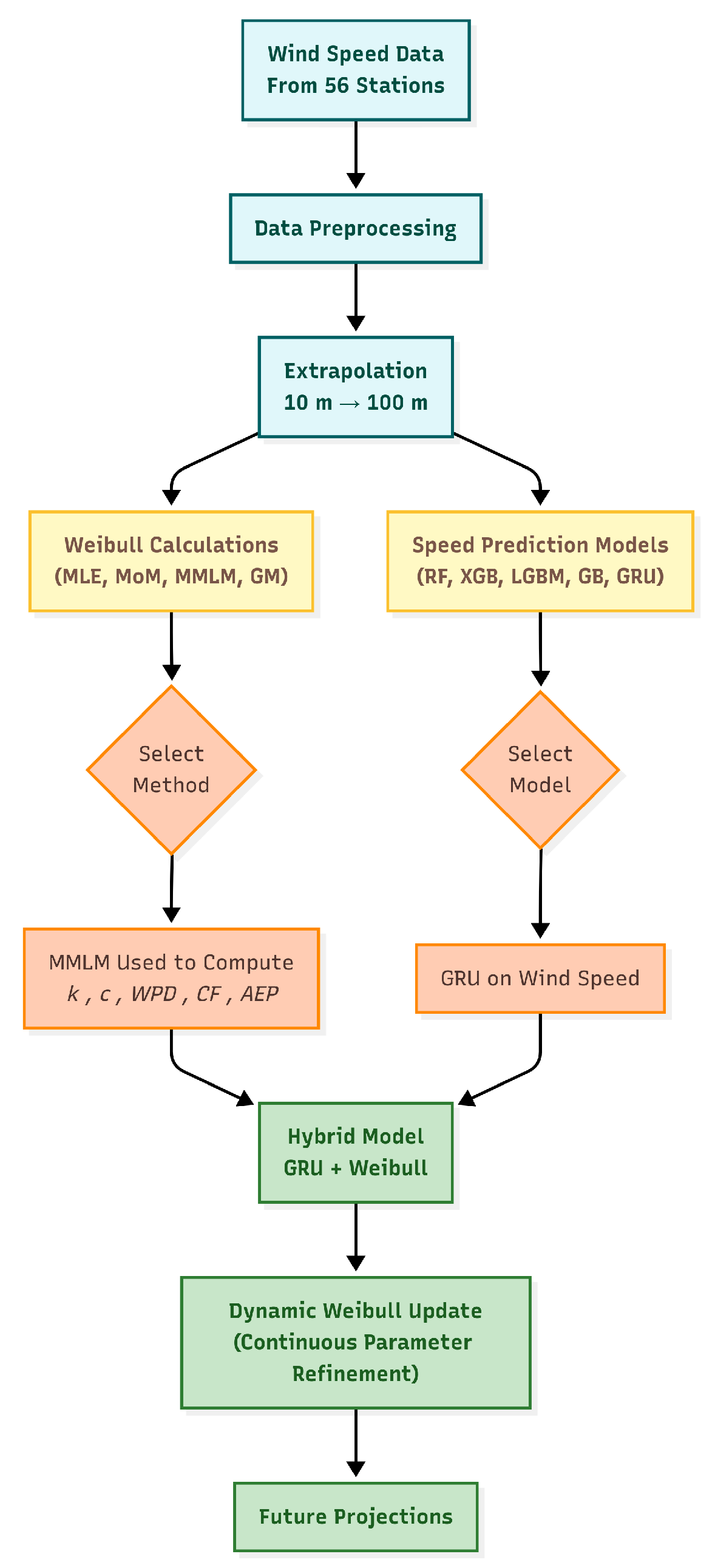
In this study, statistical analysis of wind speeds at 56 locations representing Turkey’s seven geographical regions was conducted using the Weibull distribution. Wind speed data measured at 10 m height over a five-year period spanning from 2020 top 2024 were obtained from the Turkish State Meteorological Service. These data were extrapolated to 100 m height, with the operational height of wind turbines being taken into account. During the analysis process, Weibull distribution parameters were estimated for each location using various statistical methods. These methods included MLE, MoM, modified maximum likelihood method (MMLM), and GM. Following comparisons, the MMLM was identified as the approach providing the highest fit. Utilizing the Weibull parameters calculated via this method, we derived the wind power density ($WPD$) and characteristic wind speeds. Additionally, performance indicators such as $CF$ and $AEP$ were computed for all locations using three selected wind turbine models. For future-oriented forecasts, wind speed predictions were generated with five ML models (LightGBM, XGBoost, RF, gradient boosting, and GRU); their performances were assessed through $RMSE$, mean absolute error ($MAE$), and mean absolute percentage error ($MAPE$) metrics. The GRU model, which demonstrated superior performance by effectively capturing time series dynamics, was hybridized with the Weibull distribution to produce projections for 2025, and the accuracy of this hybrid approach was analyzed. $WPD$ values based on hybrid model predictions were compared with existing Weibull-based $WPD$ results. The diagram visualizing the methodological flow of the study is presented in Figure 1. This flowchart systematically illustrates the stages encompassing data collection, preprocessing, statistical modeling, and ML integration undertaken to evaluate Turkey’s onshore wind energy potential.

2. Materials and Methods

2.1. Collection and Preprocessing of Wind Data

The accurate and effective evaluation of wind energy potential necessitates, as the most fundamental and priority step, the identification of suitable regions for collecting meteorological data such as wind speed and direction. In this study, location selection was conducted to reflect Turkey’s diverse geographical, topographical, and climatic conditions, particularly for determining Weibull parameters. During the location selection process, to more robustly represent the regional distribution of wind energy potential in Turkey, data from the Wind Energy Potential Atlas (REPA) were considered as preliminary information [28]. In the selection process, emphasis was placed on encompassing all seven geographical regions of Turkey, balancing coastal and inland areas, incorporating varying elevation levels, and including regions with high wind potential or those exhibiting promising potential. Consequently, the acquired data more accurately represented Turkey’s overall wind regime and enhanced the national generalizability of the results. Simultaneously, the objective was to elucidate key characteristics such as the spatial distribution, continuity, and variability of wind energy resources.

Within the scope of this study, hourly wind speed data measured over a five-year period from 1 January 2020 to 31 December 2024, at selected land stations were analyzed. The data were provided by the General Directorate of Meteorology, with all measurements conducted using anemometers positioned at a height of 10 m above ground level. This height is the standard level accepted in meteorological observations. The accuracy and reliability of the measurement instruments employed are critical factors directly influencing data quality. Accordingly, calibrations of all anemometers at the Meteorological Service are performed at regular intervals by the Turkish Accreditation Institution (TÜRKAK) in compliance with the TS EN ISO/IEC 17025 standard [29]. This practice ensures the data’s adherence to international quality standards [30]. The names of the stations selected for the study, along with their cities and regional locations, are presented in

Table 1. Stations with city and region information.

No	Station	City	Region
1	Gelibolu	Canakkale	Marmara
2	Kepsut	Balikesir	Marmara
3	Gokceada	Canakkale	Marmara
4	Bandırma	Balikesir	Marmara
5	Silivri	Istanbul	Marmara
6	Catalca	Istanbul	Marmara
7	Lalapasa	Edirne	Marmara
8	Sarkoy	Tekirdag	Marmara
9	Canakkale	Canakkale	Marmara
10	Karacabey	Bursa	Marmara
11	Vize	Kirklareli	Marmara
12	Armutlu	Yalova	Marmara
13	Geyve	Sakarya	Marmara
14	Sile	Istanbul	Marmara
15	Kandira	Kocaeli	Marmara
16	Kirklareli	Kirklareli	Marmara
17	Bozuyuk	Bilecik	Marmara
18	Mesudiye	Ordu	Black Sea
19	Tokat	Tokat	Black Sea
20	Ladik	Samsun	Black Sea
21	Gerze	Sinop	Black Sea
22	Bafra	Samsun	Black Sea
23	Merzifon	Amasya	Black Sea
24	Cerkes	Cankiri	Black Sea
25	Mucur	Kirsehir	C. Anatolia
26	Gurun	Sivas	C. Anatolia
27	Yahyali	Kayseri	C. Anatolia
28	Keskin	Kirikkale	C. Anatolia
29	Uluborlu	Isparta	C. Anatolia
30	Karaman	Karaman	C. Anatolia
31	Sincik	Adiyaman	S.E. Anatolia
32	Karaburun	Izmir	Aegean
33	Soke	Aydin	Aegean
34	Alasehir	Manisa	Aegean
35	Soma	Manisa	Aegean
36	Cesme	Izmir	Aegean
37	Bodrum	Mugla	Aegean
38	Dinar	Afyonkarahisar	Aegean
39	Banaz	Usak	Aegean
40	Ayvalik	Balikesir	Aegean
41	Bergama	Izmir	Aegean
42	Akhisar	Manisa	Aegean
43	Babadag	Denizli	Aegean
44	Arapgir	Malatya	E. Anatolia
45	Guroymak	Bitlis	E. Anatolia
46	Taslicay	Agri	E. Anatolia
47	Aydintepe	Bayburt	E. Anatolia
48	Karliova	Bingol	E. Anatolia
49	Gevas	Van	E. Anatolia
50	Caglayancerit	K.Maras	Mediterranean
51	Samandag	Hatay	Mediterranean
52	Nurdagi	Gaziantep	Mediterranean
53	Mut	Mersin	Mediterranean
54	Iskenderun	Hatay	Mediterranean
55	Feke	Adana	Mediterranean
56	Bahce	Osmaniye	Mediterranean

.

Datasets collected from 56 meteorological stations were subjected to comprehensive preprocessing procedures. Missing values were handled contextually based on subsequent analytical requirements; they were either preserved as “not a number” (NaN) or filled via linear interpolation. Duplicate records and erroneous data points were systematically removed to ensure data integrity. For the integration of ML models, wind direction data were transformed into angular representation formats. Time data were converted to timestamp formats, and sine and cosine transformations were applied to capture periodic patterns. Additionally, a custom location dataset was compiled, containing information on the region, province, latitude, longitude, and elevation for the stations.

2.2. Extrapolation of Wind Speeds

In wind energy potential analyses, due to the variability of wind speeds with height from the ground, the measured data must be adapted to the turbine hub height. This adaptation process is performed using the power law approach, which defines the relationship between wind speed and height. This method enables parametric modeling of how wind speed changes with height, taking into account friction effects [31,32]. In the power law model, the friction coefficient, also known as the Hellman exponent ($\alpha$), is an empirical constant determined based on terrain roughness. This coefficient typically ranges between 0.10 and 0.40 [7,33]. In this study, wind speed extrapolation from the measurement height to the turbine hub height was conducted using $\alpha$ = 0.25. The power law approach is expressed by the following mathematical formula:

$$v=v_0{\left({\displaystyle \frac{h}{h_0}}\right)}^{\alpha }$$

(1)

where v and $v_0$ are the wind speeds at heights h and $h_0$, respectively, and $\alpha$ is the power-law coefficient.

2.3. Weibull Parameters

The Weibull function is one of the most accurate and widely used distribution functions for describing wind speed data. The Weibull distribution is typically employed with two parameters: the scale and shape parameters [34]. The scale parameter provides information about the site’s characteristic average wind speeds, while the shape parameter indicates the sharpness of the distribution. However, in some cases, a three-parameter Weibull distribution is also utilized; this model includes an additional location parameter [35]. The two-parameter model yields good results with a limited number of parameters, whereas the three-parameter model can better capture shifts in the dataset [36]. The definition of the two-parameter Weibull distribution is as follows [7,37,38]:

$$f\left(v\right)={\displaystyle \frac{k}{c}}{\left({\displaystyle \frac{v}{c}}\right)}^{k-1}exp\left[-{\left({\displaystyle \frac{v}{c}}\right)}^k\right]$$

(2)

Here, $f\left(v\right)$ represents the probability of observing wind speed v, c is the Weibull scale parameter, and k is the Weibull shape parameter. To determine the energy potential, the Weibull parameters must be identified, and these parameters can be obtained using various methods.

2.3.1. Maximum Likelihood Estimation—MLE

MLE is a statistical approach that maximizes the likelihood function to find the parameters best fitting the dataset [39]. For n observations $v_1,v_2,\dots ,v_n$, the likelihood function is defined as the product of the density functions mentioned above. The parameters are found at the point where the derivatives of the log-likelihood function equal zero [10,40]. The equations used for this method are as follows:

$$k={\left({\displaystyle \frac{{\displaystyle \sum _{i=1}^n{v}_i^{k}ln\left(v_i\right)}}{{\displaystyle \sum _{i=1}^n{v}_i^k}}}-{\displaystyle \frac{{\displaystyle \sum _{i=1}^{n}ln\left(v_i\right)}}{n}}\right)}^{-1}$$

(3)

In this equation, $v_i$ represents the observations, and the shape parameter k is estimated using iterative methods (e.g., Newton–Raphson). The equation is derived by setting the derivative of the log-likelihood function with respect to k to zero, enabling parametric estimation. The scale parameter c is estimated using the following formula:

$$c={\left({\displaystyle \frac{1}{n}}\sum _{i=1}^n{v}_i^k\right)}^{{\displaystyle \frac{1}{k}}}$$

(4)

This equation calculates c by taking the k-th root of the average of the k-th powers of the observations. The set of equations is typically solved using numerical methods.

2.3.2. Method of Moments—MoM

MoM is a commonly used parametric method for estimating Weibull distribution parameters. In this approach, the theoretical moments of the distribution are equated to the sample moments to estimate the shape (k) and scale (c) parameters [41,42]. The theoretical mean of the Weibull distribution is expressed as follows:

$$\overline{v}=c\Gamma \left(1+{\displaystyle \frac{1}{k}}\right)$$

(5)

In this equation, $\Gamma (·)$ denotes the Gamma function. After the shape and scale parameters are estimated, the theoretical standard deviation (S) of the distribution is calculated as follows:

$$S=c\sqrt{\Gamma \left(1+{\displaystyle \frac{2}{k}}\right)-{\left[\Gamma \left(1+{\displaystyle \frac{1}{k}}\right)\right]}^2}$$

(6)

This formula is obtained as the square root of the variance and reflects the spread of the distribution. Additionally, the following equations are used to calculate the sample moments. The sample mean is calculated as follows:

$$\overline{v}={\displaystyle \frac{1}{n}}\sum _{i=1}^n{v}_i$$

(7)

The sample standard deviation is calculated as follows:

$$S=\sqrt{{\displaystyle \frac{1}{n-1}}\sum _{i=1}^n{\left(v_i-\overline{v}\right)}^2}$$

(8)

These two sample moments enable parameter estimation by equating them to the theoretical moments. MoM offers a practical and computationally straightforward alternative for parametric estimation, particularly in small samples. However, the method may be susceptible to sensitivity loss when the shape parameter is low due to increasing discrepancies between theoretical and sample moments.

2.3.3. Modified Maximum Likelihood Method—MMLM

The MMLM is a variation of MLE, designed to enhance computational efficiency, particularly for small datasets. This method provides more robust estimates by incorporating a weighting factor (e.g., $f\left(v_i\right)$) into the likelihood function [11,43,44]. The equations used are as follows:

$$k={\left({\displaystyle \frac{{\displaystyle \sum _{i=1}^N{v}_i^{k}ln\left(v_i\right)f\left(v_i\right)}}{{\displaystyle \sum _{i=1}^N{v}_i^{k}f\left(v_i\right)}}}-{\displaystyle \frac{{\displaystyle \sum _{i=1}^{N}ln\left(v_i\right)f\left(v_i\right)}}{f(v\ge 0)}}\right)}^{-1}$$

(9)

In this equation, $f\left(v_i\right)$ represents the values of the density function at the observations, while $f(v\ge 0)$ denotes the normalization factor for positive speeds. The scale parameter is as follows:

$$c={\left({\displaystyle \frac{1}{f(v\ge 0)}}\sum _{i=1}^N{v}_i^{k}f\left(v_i\right)\right)}^{{\displaystyle \frac{1}{k}}}$$

(10)

2.3.4. Graphical Method—GM

To estimate the parameters of the Weibull distribution (shape parameter k and scale parameter c) using GM, a logarithmic transformation is applied to the cumulative distribution function [45,46,47].

$$ln\left[-ln(1-F(v\left)\right)\right]=kln\left(v\right)-kln\left(c\right)$$

(11)

This method facilitates the easy derivation of parameters using linear regression techniques. The transformation begins by determining approximate $F\left(v\right)$ values based on the dataset; these values are typically calculated using ordered statistics (e.g., the median rank method). Subsequently, x and y values are derived to create a scatter plot, and regression coefficients are estimated using the least squares method.

$$y={\beta }_0+{\beta }_{1}x$$

(12)

The shape parameter k defines the structure of the distribution, while the scale parameter c determines its scale. This approach is particularly preferred for small datasets or situations where numerical optimization is challenging.

$$k={\beta }_1$$

(13)

$$c=e^{-{\displaystyle \frac{{\beta }_0}{{\beta }_1}}}$$

(14)

2.4. Power Density ($WPD$)

The power of the wind that flows at a speed (v) through an area swept by the rotor (A) can be expressed by the following equations [48]:

$$P\left(v\right)={\displaystyle \frac{1}{2}}\rho v^{3}A$$

(15)

where $\rho$ is the air density in kg/m³, usually taking values between 1.18 kg/m³ and 1.27 kg/m³ [49]. The specific value used in this study was 1.225 kg/m³.

The $WPD$ using the Weibull probability density function can be calculated as follows [48]:

$$WPD={\displaystyle \frac{P}{A}}={\displaystyle \frac{1}{2}}\rho {\int }_0^{\infty }{v}^3{f}_w\left(v\right)dv={\displaystyle \frac{1}{2}}\rho c^3\Gamma \left(1+{\displaystyle \frac{3}{k}}\right)$$

(16)

2.5. Characteristic Wind Speeds ($V_{mp}$ and $V_{maxe}$)

The Weibull distribution also enables the quantitative determination of two important characteristic wind speeds: the most probable wind speed ($V_{mp}$) and the wind speed carrying the maximum energy ($V_{maxe}$) [35,50].

$$V_{mp}=c{\left(1-{\displaystyle \frac{1}{k}}\right)}^{k-1}$$

(17)

$$V_{maxe}=c{\left(1+{\displaystyle \frac{2}{k}}\right)}^{k-1}$$

(18)

2.6. Capacity Factor ($CF$) and Annual Energy Production ($AEP$)

Energy production and $CF$ from wind turbines are fundamental indicators for evaluating the performance of a wind energy project. Energy production refers to the total amount of electricity generated by the turbine over a specific time period, while the $CF$ represents the ratio of actual production to the turbine’s maximum theoretical production capacity. These parameters are calculated with wind speed data, turbine power curves, and operational limits being taken into account. Accurate estimation of energy production and $CF$ is critically important for economic analyses and investment decisions.

The $AEP$ of a wind turbine is the total amount of electrical energy expected to be produced over a year and can be obtained as follows [51]:

$$AEP={\int }_0^{\infty }{P}_w(V,\rho )f\left(V\right)8760dV$$

(19)

Here, $f\left(V\right)$ denotes the wind speed probability density, while $P_w(V,\rho )$ represents the turbine’s specific power curve and can be calculated using Equation (20) [51,52]:

$$P_w={\displaystyle \frac{1}{2}}\rho A{v}^3{C}_p$$

(20)

Here, $C_p$ is the power coefficient (dimensionless, with a maximum theoretical limit of approximately 0.593—Betz limit) representing the efficiency of the wind turbine [7].

The $CF$ provides the ratio between the energy actually produced by a wind turbine and the energy it could theoretically produce at maximum capacity and can be obtained as follows [53]:

$$CF={\displaystyle \frac{AEP}{P_{rated}·T}}$$

(21)

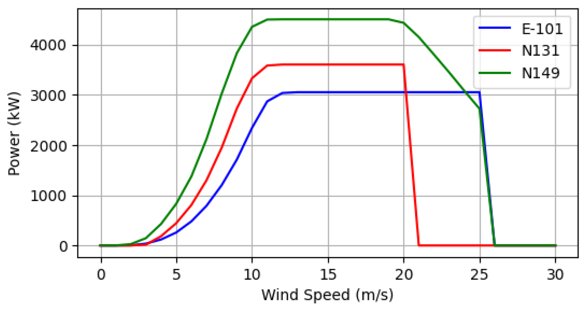
Here, $P_{rated}$ denotes the turbine’s rated power, and T represents the time period. The specific parameters for the turbines selected in this study are detailed in

Table 2. Wind power turbine model specifications.

Specification	Enercon	Nordex	Nordex
	E-101	N131	N149
Rated power (MW)	3.05	3.6	4.5
Hub height (m)	99	106	105
Cut-in (m/s)	2	3	3
Rated (m/s)	13	11	11
Cut-out (m/s)	25	20	26
Rotor diameter (m)	101	131	149.1

, and the power curves of the turbines are shown in Figure 2 [54].

The E-101 model developed by Enercon is specifically designed for onshore wind farms and features a rotor diameter of 101 m. It is optimized to deliver high efficiency in low-to-medium wind speed conditions. Nordex’s N131 model, with its expansive 131 m rotor diameter, enables high energy production even at low wind speeds. An advanced version, the Nordex N149, stands out with its larger rotor diameter of 149 m and higher power capacity. Equipped with enhanced control systems, the N149 offers superior adaptability to variable wind conditions.

2.7. Machine Learning Models for Wind Speed Prediction

The planning of wind energy potential holds critical importance for the sustainability of renewable energy systems. To predict wind speed, five ML models were employed: LightGBM, XGBoost, RF, gradient boosting, and GRU. These models were selected due to their robustness in handling time series data and regression tasks. They facilitate the capture of temporal dependencies and nonlinear patterns in wind speed measurements through recurrent structures.

• LightGBM: LightGBM is a gradient boosting framework that enables efficient tree construction using histogram-based algorithms, providing faster training and higher accuracy on large datasets. It incorporates leaf-wise tree growth and exclusive feature bundling, with regularization parameters such as learning rate and maximum depth minimizing overfitting while reducing computational load [55].
• XGBoost: XGBoost is a distributed gradient boosting library optimized for scalability and performance. It sequentially builds an ensemble of decision trees, optimizing a regularized objective function that includes both loss terms and model complexity penalties. Key hyperparameters such as subsample ratio and column subsampling enhance generalization in structured data such as meteorological time series [56].
• RF: RF is an ensemble method that constructs multiple decision trees using bootstrap aggregation (bagging) and random feature selection at each split. This approach reduces variance and overfitting by averaging predictions across uncorrelated trees; it is suitable for capturing complex interactions in wind speed features and requires minimal hyperparameter tuning [57].
• Gradient Boosting: Gradient boosting iteratively trains weak learners (typically decision trees) to correct residual errors from previous models, minimizing differentiable loss functions such as mean squared error. It employs shrinkage (learning rate) and subsampling to control each tree’s contribution; it provides a flexible framework for regression problems in environmental data forecasting [58].
• GRU: GRU is a variant of the recurrent neural network optimized for sequential data; it incorporates update and reset gates to manage long-term dependencies and mitigate vanishing gradient issues. In this study, GRU layers were stacked to process time-lagged wind speed sequences; hyperparameters such as the number of hidden units and dropout rates were tuned to effectively model temporal autocorrelations [59].

2.8. Hybrid (Weibull–MultiStep GRU) Model for Projections

To extend multistep forward forecasting capabilities and incorporate probabilistic elements suitable for wind energy applications, a hybrid approach was developed that integrates multistep GRU predictions with Weibull distribution-based sampling. This method addresses seasonal trends and uncertainties in projections in which wind speed typically follows a Weibull distribution. The multistep GRU forecast iteratively predicts future sequences leveraging the network’s recurrent nature. Given hourly wind speed data, the model is trained on input sequences of length T and predicts future steps H.

The update of the hidden state in a standard GRU cell is governed as follows [60]

$${\mathbf{z}}_t=\sigma ({\mathbf{W}}_{xz}{\mathbf{x}}_t+{\mathbf{W}}_{hz}{\mathbf{h}}_{t-1}+{\mathbf{b}}_z)$$

(22)

$${\mathbf{r}}_t=\sigma ({\mathbf{W}}_{xr}{\mathbf{x}}_t+{\mathbf{W}}_{hr}{\mathbf{h}}_{t-1}+{\mathbf{b}}_r)$$

(23)

$${\tilde{\mathbf{h}}}_t=tanh({\mathbf{W}}_{xh}{\mathbf{x}}_t+{\mathbf{W}}_{hh}({\mathbf{r}}_t\odot {\mathbf{h}}_{t-1})+{\mathbf{b}}_h)$$

(24)

$${\mathbf{h}}_t=(1-{\mathbf{z}}_t)\odot {\mathbf{h}}_{t-1}+{\mathbf{z}}_t\odot {\tilde{\mathbf{h}}}_t$$

(25)

where ${\mathbf{x}}_t$ denotes the input at time t; ${\mathbf{h}}_t$, the hidden state; ${\mathbf{z}}_t$ and ${\mathbf{r}}_t$, the update and reset gates, respectively; $\sigma$, the activation of the sigmoid; tanh, the hyperbolic tangent; and ⊙, the element-wise multiplication. For multistep forecasting, predictions are generated autoregressively: the output at each step serves as input for the next, enabling forward projections from hourly data (e.g., for daily or weekly horizons).

The hybrid projection combines the deterministic output of the multistep GRU with a stochastic component derived from the Weibull mean, weighted by an adjustable parameter $\alpha$$(0\le \alpha \le 1)$ that balances model dependency and distributional adjustment. The projection equation is formalized as follows:

$${\mathrm{Projection}}_t=\alpha ·\mathrm{GRU}{\mathrm{Pred}.}_t+(1-\alpha )·{\mathrm{Weibull}}_{mean}$$

(26)

Here, the GRU prediction represents the multistep forecast from the recurrent network trained to produce sequences over extended horizons (e.g., hourly steps for daily or weekly projections). The Weibull mean accounts for the expected value under the assumed distribution, enhancing robustness against outliers and seasonal variability. The Weibull mean, represented by Equation (5), is numerically calculated using the gamma function for k and c estimated from historical data using the MMLM method. This hybrid framework preserves initial values, safeguards against seasonal trends, and facilitates long-term projections through iterative sampling from the Weibull distribution during GRU inference.

2.9. Evaluation Metrics

Numerous evaluation metrics have been developed and applied to assess the accuracy of forecasting models, yet none has emerged as a universally adopted benchmark. Common indicators for gauging predictive efficacy include $RMSE$, $MAE$, $MAPE$, and the coefficient of determination ($R^2$). These measures are widely used in deterministic forecasting scenarios to quantify the deviations between predicted and observed values. For short-term wind speed prediction, $RMSE$ is frequently selected as the primary benchmark for method comparisons due to its sensitivity to significant errors, as evidenced in previous studies [61,62].

This section presents the mathematical formulations of key metrics ($MAE$, $RMSE$, $MAPE$, and $R^2$) to provide a robust framework for model selection and result analysis. The equations are as follows:

$$MAE={\displaystyle \frac{1}{n}}\sum _{i=1}^n|y_t-{\widehat{y}}_t|$$

(27)

$$RMSE=\sqrt{{\displaystyle \frac{1}{n}}\sum _{i=1}^n{(y_t-{\widehat{y}}_t)}^2}$$

(28)

$$MAPE={\displaystyle \frac{1}{n}}\sum _{i=1}^n\left|{\displaystyle \frac{y_t-{\widehat{y}}_t}{y_t}}\right|$$

(29)

$$R^2=1-{\displaystyle \frac{{\sum }_{i=1}^n{(y_t-{\widehat{y}}_t)}^2}{{\sum }_{i=1}^n{(y_t-\overline{y})}^2}}$$

(30)

In the equations, $y_t$ represents the actual value observed at time t, ${\widehat{y}}_t$ denotes the predicted value at time t, and $\overline{y}={\displaystyle \frac{1}{n}}{\sum }_{t=1}^n{y}_t$ is the mean of the dataset, where n is the total number of observations.

These metrics enable a comprehensive evaluation of forecasting accuracy, with $MAE$ and $MAPE$ providing insights into absolute and relative errors, $RMSE$ emphasizing larger deviations, and $R^2$ assessing the proportion of variance explained by the model.

2.10. Hyperparameters for Hybrid GRU–Weibull

Table 3. Model Hyperparameters for GRU and Hybrid GRU–Weibull.

Model	Hyperparameter	Value
GRU	Architecture	Sequential: GRU → Dense
GRU	GRU units	128
GRU	GRU activation	tanh
GRU	Input shape	(24 h, 7 features)
GRU	Dense units	4320 (1 month hourly)
GRU	Optimizer	Adam
GRU	Loss function	MSE
GRU	Epochs	30
GRU	Batch size	512
GRU	Prediction length (PRED_LEN)	4320 h
HGW	GRU component	Same as GRU model
HGW	Weibull estimation method	MMLM
HGW	Weibull parameters	k_hist, c_hist
HGW	Trend smoothing	24 h rolling mean

presents the hyperparameters of two models employed for wind speed forecasting: a gated recurrent unit (GRU) neural network and a hybrid GRU–Weibull model. The GRU model is a sequential deep learning architecture designed for multi-step time-series prediction, while the hybrid GRU–Weibull model integrates GRU predictions with Weibull distribution-based projections to enhance forecasting robustness.

This implementation was carried out using Google Colab, leveraging its computational resources for model training and evaluation. The table summarizes key architectural and training parameters for the GRU model, including layer configurations, optimizer, and sequence lengths. For the Hybrid GRU–Weibull model, it details the GRU component (identical to the standalone GRU model) and the Weibull estimation methodology, including parameter estimation and post-processing techniques. This representation facilitates comparison of model configurations for reproducibility and further analysis.

3. Results and Discussion

In this study, five years of wind data from 2020 to 2024 were analyzed from 56 meteorological stations in Turkey. The data were collected at 10 m height and extrapolated to 100 m. For locations representing seven geographical regions, Weibull parameters were obtained using the MMLM, which provided the highest $R^2$ fit. These parameters were used to calculate $WPD$, characteristic wind speeds ($V_{mp}$ and $V_{maxe}$), $AEP$, and $CF$ for the 56 locations. Based on the obtained data, ML approaches (LightGBM, XGBoost, RF, gradient boosting, and GRU) were applied to perform wind speed predictions; GRU exhibited the superior performance. Accordingly, the multistep GRU model was hybridized with the Weibull distribution, with deterministic forecasts being integrated with stochastic components to more effectively manage seasonal trends and uncertainties in long-term projections.

3.1. Wind Speed Profiles and Weibull Parameter Analysis

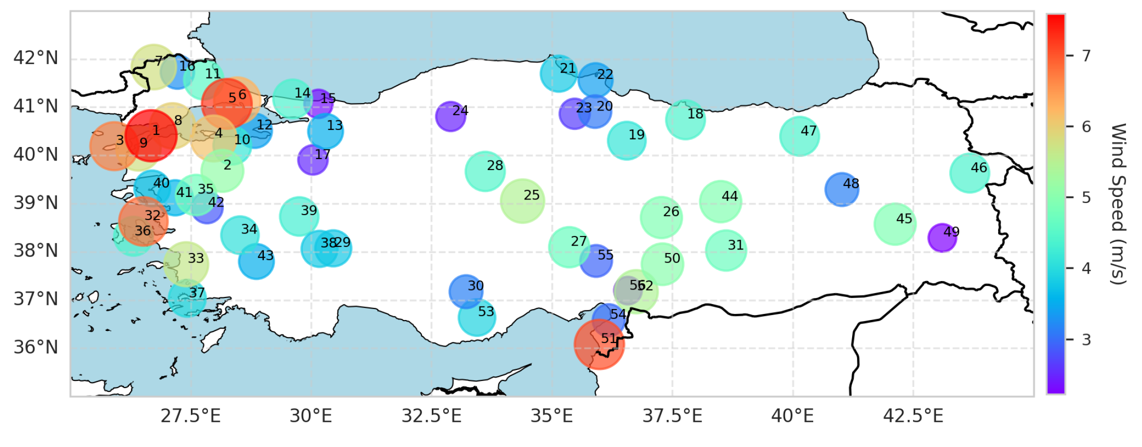
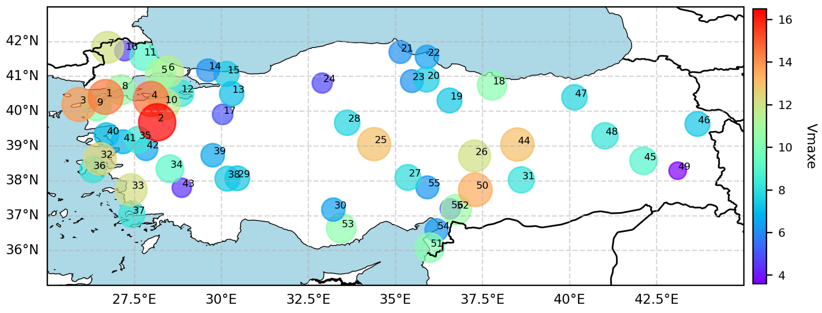
The five-year average wind speed distribution presented in Figure 3 clearly reflects the geographical diversity of Turkey’s wind regimes. Coastal areas in the Marmara and Aegean regions, particularly locations such as Gelibolu (7.59 m/s), Silivri (7.20 m/s), Samandağ (7.05 m/s), and Karaburun (6.82 m/s), stand out with high wind speeds. These regions are influenced by open-sea winds from the Marmara and Aegean seas. Gelibolu and Karaburun, situated in the wind corridor functions of the Çanakkale Strait and Aegean, regularly receive high-speed winds. Samandağ, due to its Mediterranean coastal position, benefits from a combination of coastal flatness and sea breezes, resulting in strong and consistent wind flows. In contrast, locations in the interior and eastern regions, such as Bahce (2.23 m/s), Gevaş (2.23 m/s), and Kandıra (2.34 m/s), exhibit low wind speeds. This indicates that wind flow is limited by topographical barriers in the Taurus Mountains, around Lake Van, and in the rugged interior of the Black Sea region. Overall, western and northwestern coastal areas provide advantages for energy production with high wind speeds, while interior and mountainous regions possess limited wind potential.

To ensure the analytical depth and regional representation of the study, 12 locations (Gelibolu, Çatalca, Mut, Karaburun, Sıncık, Mucur, Bandırma, Çağlayancerit, Arapgir, Söke, Mesudiye, Yahyalı) were selected from the initial 56 locations. These locations reflect the regional distribution of Turkey’s wind energy potential and contribute to simplifying the academic narrative in certain modeling and visualization processes.

Wind direction is a critical parameter in the assessment of the potential for wind energy and is as important as wind speed. Accurately determining the dominant wind direction enables optimal turbine placement for maximum efficiency, directly enhancing energy production. It also helps minimize wake effects between turbines, which can reduce speed and increase turbulence for downstream units, thereby lowering output. Given that the wind direction varies seasonally and regionally, long-term orientation-based analyses are essential for sustainable energy planning. Additionally, turbine blades and towers are designed to withstand wind loads from specific directions, making wind direction a key factor for safe engineering practices. Consequently, this study incorporated wind direction analysis and integrated it into the evaluations.

The wind rose diagrams generated for the 12 locations visualize direction-based wind regimes, supporting the distinction between coastal and interior regions (Figure 4). Gelibolu, Bandrma, and Atalca reflect the character of the wind corridor of Marmara with strong and dominant winds from the northeast (NE) direction. In Gelibolu, the dominant wind direction is northeast-north (NE-N), prevailing with approximately 20–25% frequency. Similarly, in Bandırma, the NE-N direction stands out with 31% frequency, while in Çatalca, this direction is dominant at 23%, with a consistent unidirectional pattern accompanied by moderate speeds. In Karaburun, the dominant wind direction is again NE-N, prevailing with 32% frequency. On the other hand, some locations exhibit more scattered wind directions.

For instance, in Mesudiye, winds blow from various directions between south (S) and NE-N, without a distinct dominant direction. In Mut, the dominant wind direction is northwest–north (NW-N), prevailing with 30% frequency, reflecting a stable but relatively low-speed wind pattern. In Yahyalı, the dominant direction is shared between southeast–south (SE-S) and its opposite, NW-N, indicating a lack of clear orientation and an irregular wind regime. In general, locations such as Mesudiye, Alayancerit, Arapgir, and Yahyal exhibit scattered patterns in the wind direction. In these regions, winds blow from various directions extending from south to north, which is typically associated with environmental factors such as complex topographical structures, mountainous terrain effects, and variable atmospheric conditions.

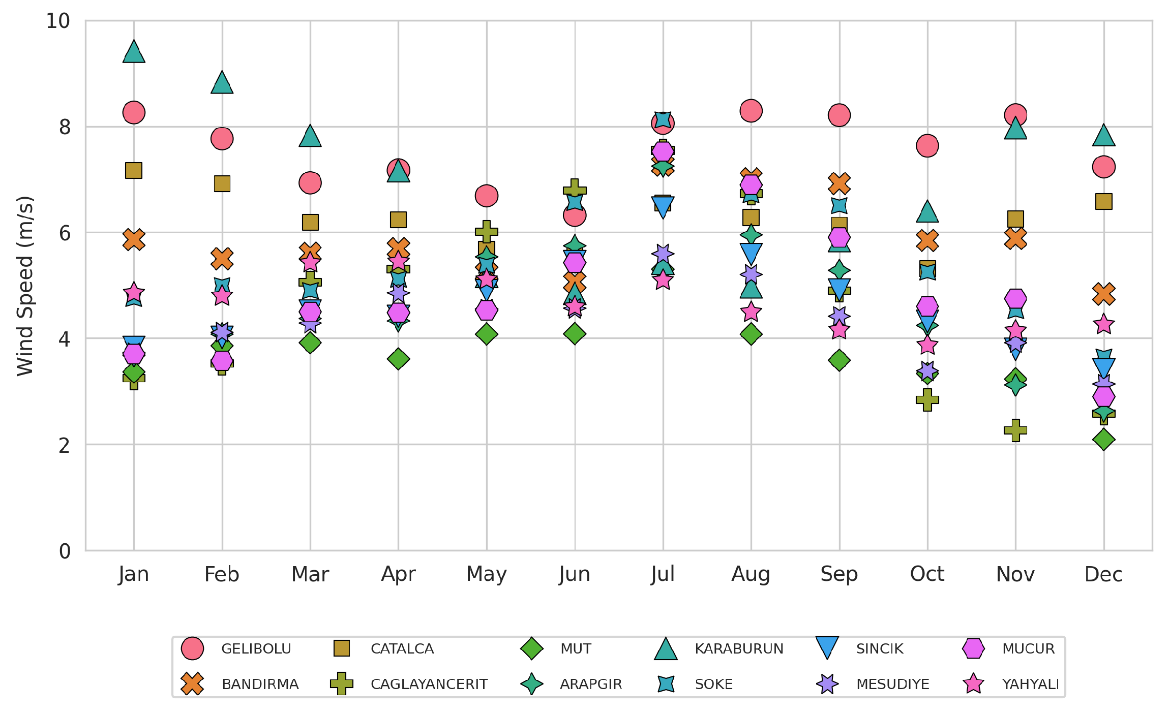
Figure 5 presents the monthly average wind speed distribution for the selected 12 locations. For each month, averages of wind speed data from January, February, March, and other months over five years were calculated to analyze inter-location and seasonal differences. This approach enabled a month-based analysis of long-term wind behaviors. The graph indicates that the wind speeds exhibit distinct seasonal variations. During winter months (January, February, November, and December), wind speeds show a marked increase; particularly in coastal locations such as Gelibolu, Karaburun, and Söke, speeds reach 8–10 m/s levels.

In summer months (June, July, August), a general decrease in wind speeds was observed. This decline was more pronounced in interior locations such as Mut and Çatalca, with speeds dropping to 2–3 m/s in some months. During spring and autumn months (particularly April, May, September, and October), moderate increases in wind speeds were noted; values in the 4–8 m/s range were noteworthy in transitional regions such as Bandırma and Çağlayancerit. Additionally, the role of topographical effects on wind speeds was clearly evident. In mountainous stations such as Mesudiye and Yahyalı, wind speeds peaked at 6–8 m/s, especially during the winter months.

The graphs presented in Figure 6 include histograms based on wind speed data for 12 locations and probability density functions obtained using four Weibull methods (MLE, MoM, MMLM, GM). In the evaluation based on the values of $R^2$, the MMLM method achieved the highest fit values in all locations and demonstrated the best overlap with the histograms; for example, an exceptional value of $R^2$ of 0.999 was obtained in Bandırma. This underscores that MMLM is the most reliable option for modeling wind speed distributions. Furthermore, considering the varying distribution characteristics of histograms across locations, the consistent performance of MMLM led to its determination as the optimal Weibull approach aligned with the study’s objectives. Therefore, in this study, Weibull parameters were obtained using the MMLM method.

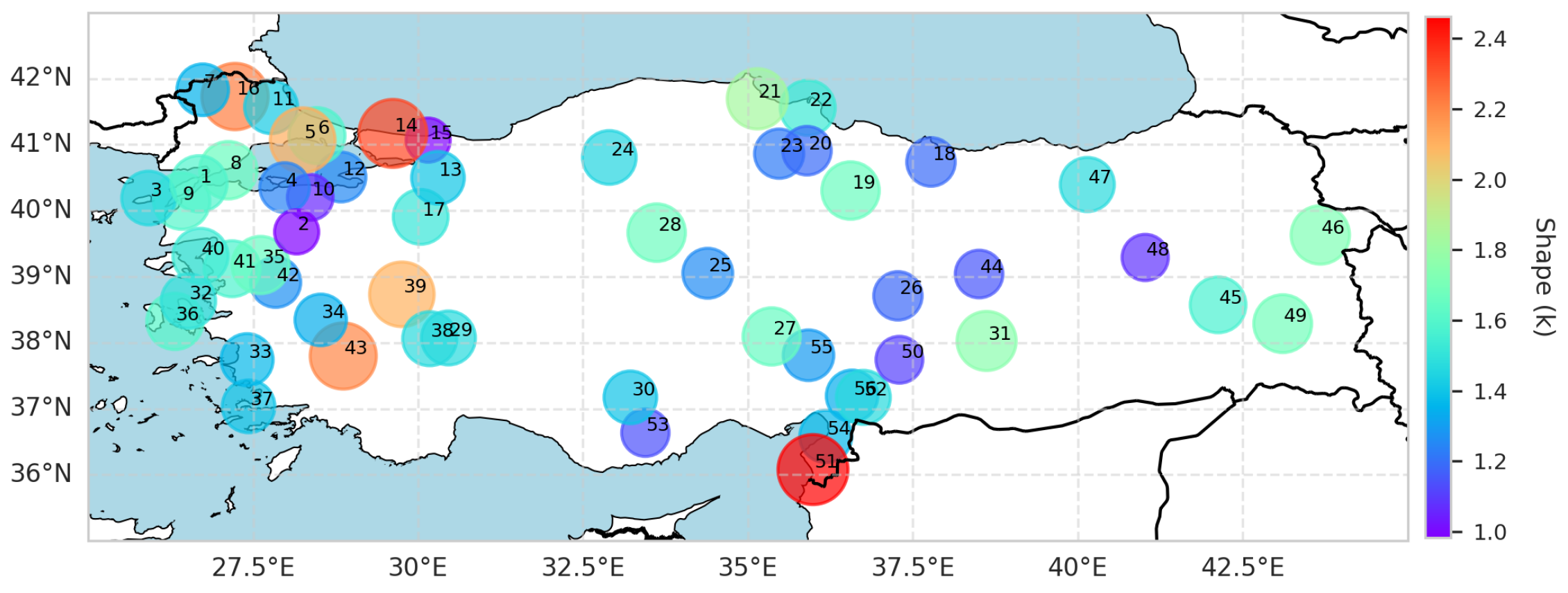
The Weibull shape parameter (k) characterizes the consistency and regularity of wind speed distributions. The k parameters calculated for 56 locations in this study are visualized on a map of Turkey in Figure 7. Locations such as Samandağ (2.46), Şile (2.32), and Kırklareli (2.22) exhibit high k values, indicating more predictable and regular wind regimes. The position and coastal flatness of Samandağ support this consistency. On the other hand, locations such as Karacabey (1.06), Çağlayancerit (1.11), and Mut (1.13) have notably low k values. This implies more variable and turbulent wind regimes. These locations, due to topographical diversity and mountainous terrain, display high variability in direction and speed.

The Weibull scale parameter (c) reflects the typical magnitude of wind speeds, evaluating the overall strength of the wind regime. The c parameters calculated for 56 locations in this study are visualized on a map of Turkey in Figure 8. Coastal locations such as Gelibolu (8.67 m/s), Samandağ (8.05 m/s), and Gökçeada (7.66 m/s) possess high c values, indicating strong wind regimes. This is associated with open-sea effects and geographically open orientations. Locations such as Gevaş (2.27 m/s), Bahçe (2.47 m/s), and Kandıra (2.38 m/s) stand out with low c values. Most of these locations are in mountainous or interior regions, where wind speeds are constrained by environmental barriers.

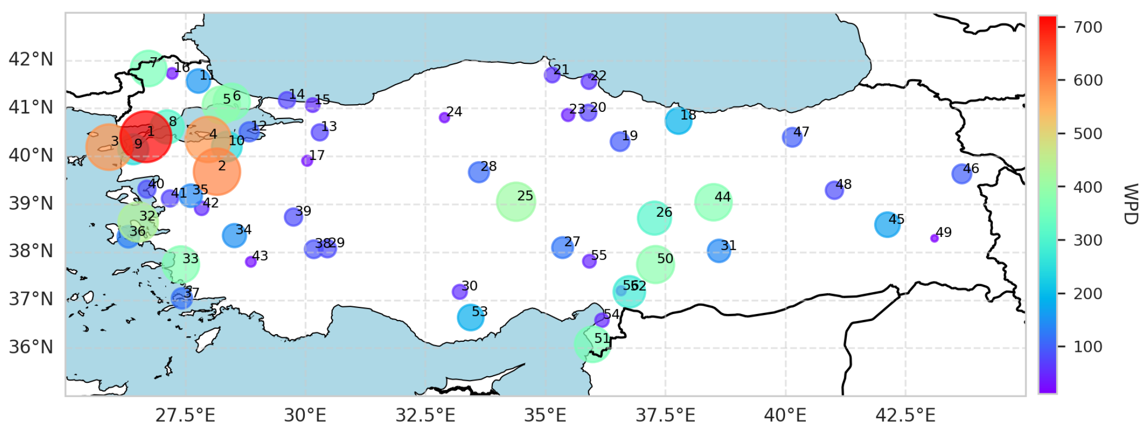
$WPD$ is a fundamental indicator of the energy potential. As shown in Figure 9, locations such as Gelibolu (721.49 W/m²), Kepsut (598.86 W/m²), and Bandrma (575.36 W/m²) exhibit values of high wind power density $WPD$, indicating significant energy potential. These locations, located in flat terrains and near coastal areas, offer the continuity and intensity of the wind favorable for energy production. In contrast, locations such as Gevaş (11.79 W/m²) and Bahçe (23.21 W/m²) provide low energy density due to topographical barriers.

Table 4. Classification based on wind power density.

Location	Speed Mean	WPD	Class
	(m/s)	(W/m2)
Gelibolu	7.59	721.49	Excellent
Kepsut	5.11	598.86	Excellent
Gokceada	6.68	579.22	Excellent
Bandırma	6.11	575.36	Excellent
Silivri	7.20	386.18	Excellent
Catalca	6.25	367.79	Good
Lalapasa	5.75	354.17	Good
Sarkoy	5.96	308.76	Good
Canakkale	5.73	251.38	Moderate
Karacabey	4.17	247.07	Moderate
Vize	4.54	154.35	Marginal
Armutlu	3.41	103.12	Poor
Geyve	3.53	73.31	Poor
Sile	4.37	73.06	Poor
Kandira	2.34	52.67	Poor
Kirklareli	3.26	31.91	Poor
Bozuyuk	2.52	27.90	Poor
Mesudiye	4.39	187.18	Marginal
Tokat	4.13	96.95	Poor
Ladik	3.08	72.04	Poor
Gerze	3.78	60.42	Poor
Bafra	3.38	60.36	Poor
Merzifon	2.65	41.85	Poor
Cerkes	2.46	23.99	Poor
Mucur	5.45	407.17	Excellent
Gurun	4.92	305.66	Good
Yahyali	4.69	121.41	Poor
Keskin	4.47	111.52	Poor
Uluborlu	3.78	83.35	Poor
Karaman	3.15	54.93	Poor
Sincik	4.71	139.98	Poor
Karaburun	6.82	433.82	Excellent
Soke	5.63	372.15	Good
Alasehir	4.08	149.10	Marginal
Soma	4.76	141.83	Poor
Cesme	4.39	130.78	Poor
Bodrum	3.98	115.76	Poor
Dinar	3.78	88.16	Poor
Banaz	4.29	82.99	Poor
Ayvalik	3.72	81.94	Poor
Bergama	3.59	73.83	Poor
Akhisar	2.84	51.16	Poor
Babadag	3.53	26.83	Poor
Arapgir	4.96	369.58	Good
Guroymak	4.93	167.86	Marginal
Taslicay	4.38	98.85	Poor
Aydintepe	4.38	98.59	Poor
Karliova	3.14	83.33	Poor
Gevas	2.23	11.79	Poor
Caglayancerit	5.02	383.18	Excellent
Samandag	7.05	356.00	Good
Nurdagi	5.42	277.47	Moderate
Mut	3.88	182.56	Marginal
Iskenderun	3.00	49.88	Poor
Feke	2.94	45.41	Poor
Bahce	2.23	23.21	Poor

presents a classification analyzing wind speed and energy potential for 56 locations. This classification is based on $WPD$ values calculated at 100 m height for each location. Based on $WPD$ values, each location is categorized into “Excellent,” “Good,” “Moderate,” “Marginal,” and “Poor” classes [63]. According to the table, eight locations fall into the “Excellent” class, while seven locations are in the “Good” class. In this evaluation based on $WPD$ values, stations with high potential (e.g., Gelibolu, Bandırma) offer ideal conditions for turbine installation, whereas stations with lower $WPD$ values (e.g., Merzifon, Bahçe) exhibit limited wind energy potential.

$V_{mp}$ represents the most frequently observed speed in the wind regime and serves as an important reference for turbine design (Figure 10). Locations such as Samandağ (6.52 m/s) and Silivri (5.85 m/s) stand out with high $V_{mp}$ values. Gelibolu’s $V_{mp}$ value is 4.64 m/s, and the significant difference between this and its average speed indicates that wind speeds are distributed across a broad spectrum in this area. This suggests the presence of low-frequency but high-energy winds. Locations such as Karlıova (0.28 m/s) and Karacabey (0.28 m/s) are notably low in terms of $V_{mp}$, indicating that winds blow both infrequently and at low speeds.

$V_{maxe}$ denotes the speeds at which wind turbines achieve the highest energy efficiency and is a critical parameter for turbine optimization (Figure 11). Locations such as Kepsut (16.51 m/s), Bandırma (14.64 m/s), and Gelibolu (14.48 m/s) exhibited high $V_{maxe}$ values, indicating substantial energy production potential. These stations are situated in coastal and flat areas where strong winds blow regularly. In interior and mountainous regions, such as Gevaş (3.61 m/s), Babadağ (4.43 m/s), and Bahçe (4.88 m/s), this value was considerably low, suggesting that the energy production capacity of wind turbines may remain limited.

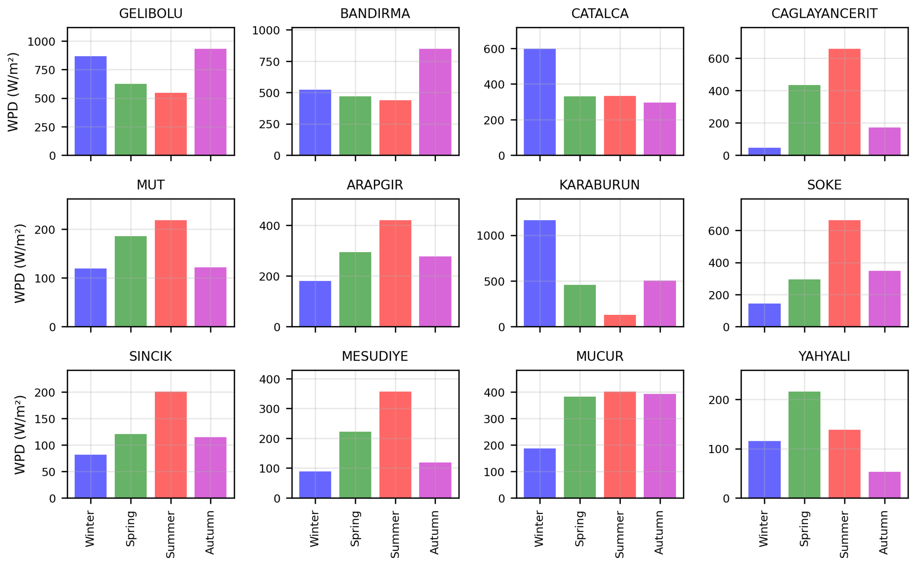
For the 12 locations, Figure 12 illustrates the seasonal variation in $WPD$. This analysis focuses on the seasonal variability of wind energy potential and highlights locations that maintain productivity in other seasons, particularly in regions with high wind speeds during winter. Overall, the winter season exhibited the highest density wind speed distribution, reflecting elevated energy potential. Karaburun is particularly noteworthy, with a $WPD$ value reaching approximately 1200 W/m² in winter, emerging as the region with the highest potential. However, the near-zero value in summer months indicates highly pronounced seasonal fluctuations in the area. Similar strong winter profiles were observed in Gelibolu and Bandırma. On the other hand, in locations such as Çağlayancerit, Mesudiye, and Sincik, $WPD$ values were notably high during summer. This suggests that wind energy can be utilized more efficiently in these regions during summer months. In locations such as Mucur and Mut, $WPD$ values remained relatively consistent across all four seasons, indicating the possibility of more stable wind energy production throughout the year. These findings underscore the importance of seasonal diversity in wind energy planning. Stations with high $WPD$ are primary candidates for wind energy development, particularly in winter. However, the variability between seasons necessitates adaptable energy management strategies to account for productivity in specific locations during summer or spring.

3.2. $CF$ and $AEP$ Analysis

Table 5. $\alpha \left(CF\right)$ and $AEP$ by location.

Location	Enercon E-101		Nordex N131		Nordex N149
	$\mathit{\alpha }\left(\mathit{CF}\right)$	$\mathit{AEP}$	$\mathit{\alpha }\left(\mathit{CF}\right)$	$\mathit{AEP}$	$\mathit{\alpha }\left(\mathit{CF}\right)$	$\mathit{AEP}$
	(%)	(MWh)	(%)	(MWh)	(%)	(MWh)
Gelibolu	37.41	9996	40.57	12,793	46.60	18,369
Kepsut	17.07	4561	20.26	6389	24.20	9540
Gokceada	31.33	8369	34.51	10,883	39.95	15,749
Bandırma	26.72	7140	29.01	9149	34.06	13,428
Silivri	31.96	8539	38.18	12,038	43.85	17,286
Catalca	26.02	6952	30.29	9553	35.20	13,877
Lalapasa	22.35	5970	25.58	8066	30.04	11,840
Sarkoy	23.96	6401	28.51	8990	33.38	13,158
Canakkale	20.21	5400	24.37	7685	28.94	11,406
Karacabey	14.30	3820	16.33	5150	19.61	7731
Vize	12.90	3447	15.88	5007	19.52	7694
Armutlu	8.62	2301	10.67	3364	13.46	5307
Geyve	6.52	1743	8.34	2630	11.06	4360
Sile	6.51	1740	8.77	2765	12.73	5016
Kandira	1.58	420	1.98	625	3.17	1250
Kirklareli	2.33	623	2.92	922	5.10	2008
Bozuyuk	2.20	586	2.81	885	4.42	1744
Mesudiye	13.27	3546	15.71	4955	19.00	7491
Tokat	8.92	2382	11.53	3636	15.14	5967
Ladik	6.13	1636	7.66	2416	9.95	3920
Gerze	5.35	1428	7.07	2228	10.14	3998
Bafra	5.38	1437	6.99	2204	9.67	3810
Merzifon	3.60	962	4.60	1449	6.38	2513
Cerkes	1.85	493	2.34	738	3.74	1475
Mucur	22.66	6054	25.41	8012	29.88	11,780
Gurun	18.14	4847	20.68	6521	24.56	9683
Yahyali	11.10	2966	14.16	4466	18.06	7120
Keskin	10.26	2739	13.17	4152	16.98	6695
Uluborlu	7.48	1999	9.57	3019	12.59	4961
Karaman	4.84	1294	6.24	1968	8.59	3386
Sincik	12.92	3452	16.48	5196	20.79	8196
Karaburun	27.41	7324	31.18	9832	36.17	14,258
Soke	23.34	6236	26.66	8406	31.23	12,309
Alasehir	12.16	3247	14.87	4689	18.28	7206
Soma	12.82	3425	16.19	5106	20.28	7995
Cesme	11.79	3150	14.91	4703	18.80	7411
Bodrum	10.03	2679	12.54	3953	15.80	6229
Dinar	7.92	2115	10.11	3189	13.21	5208
Banaz	7.62	2036	10.18	3210	14.19	5592
Ayvalik	7.42	1983	9.56	3016	12.69	5001
Bergama	6.68	1786	8.67	2735	11.72	4620
Akhisar	4.46	1191	5.69	1794	7.75	3056
Babadag	1.86	496	2.26	711	4.13	1627
Arapgir	19.60	5237	21.93	6915	26.00	10,247
Guroymak	14.54	3884	18.03	5684	22.11	8717
Taslicay	9.14	2442	11.86	3740	15.60	6150
Aydintepe	8.82	2356	11.20	3533	14.45	5695
Karliova	6.64	1775	8.14	2566	10.32	4069
Gevas	0.66	177	0.72	225	1.49	587
Caglayancerit	19.24	5140	21.38	6741	25.39	10,008
Samandag	32.32	8634	39.47	12,446	45.69	18,012
Nurdagi	20.48	5471	24.21	7635	28.60	11,274
Mut	12.55	3353	14.78	4661	17.91	7059
Iskenderun	4.36	1166	5.62	1772	7.80	3074
Feke	3.94	1052	5.05	1592	7.02	2766
Bahce	1.82	486	2.31	728	3.61	1422

presents the $CF$ and $AEP$ values calculated for three wind turbine models (Enercon E-101, Nordex N131, and Nordex N149) using the Weibull distribution on data collected from 56 wind locations in Turkey. The analysis reveals significant spatial variability arising from regional wind regimes, topographical effects, and turbine-specific performance characteristics.

In the dataset, $CF$ values range from 0.66% (Enercon E-101, Gevaş) to 46.60% (Nordex N149, Gelibolu), while $AEP$ values span from 177 MWh (Enercon E-101, Gevaş) to 18,369 MWh (Nordex N149, Gelibolu), highlighting substantial differences in wind resource quality and turbine efficiency. Gelibolu emerged as the most productive region, with $CF$ values of 37.41%, 40.57%, and 46.60% for Enercon E-101, Nordex N131, and Nordex N149, respectively, corresponding to $AEP$ values of 9996 MWh, 12,793 MWh, and 18,369 MWh. These figures reflect Gelibolu’s wind potential in the Marmara region, supported by strong and consistent winds from the Aegean and Black Sea due to its coastal position. The superior performance of Nordex N149 in Gelibolu demonstrates that its design maximizes energy capture in high wind regimes, providing an advantage over other models. Samandağ, located in the Mediterranean region, positions itself as the second-highest performing area, benefiting from coastal winds and orographic effects in the Hatay region. Bandırma, situated in the Marmara region, exhibited mid-to-high performance in $CF$ and $AEP$ values. Its proximity to the Marmara Sea ensures consistent wind exposure, maintaining it as a suitable area.

Regionally, the Marmara and Aegean regions stand out as high-performance areas. In addition to Gelibolu and Bandırma, regions such as Silivri and Gökçeada emphasize the wind energy potential of the Marmara region due to coastal exposure and favorable wind patterns. The Aegean region demonstrated strong performance in areas such as Karaburun and Söke, owing to high wind speeds and open terrain structures. In contrast, interior regions such as Central Anatolia and Eastern Anatolia generally exhibited lower $CF$ and $AEP$ values due to weaker wind resources and complex terrain.

At the lower end of performance, regions such as Gevaş and Kandıra demonstrated minimal wind energy potential due to sheltered topography or low wind speeds. Primarily located in Eastern Anatolia and the Black Sea region, these areas have limited suitability for large-scale wind energy projects, independent of turbine type. The consistently low performance across all turbines in these regions demonstrates that wind resource constraints, rather than turbine inefficiencies, constitute the primary barrier. For forecast projections, Weibull-based calculations provide a solid foundation for long-term $AEP$ and $CF$ estimates; however, region-specific factors such as wind variability, turbine maintenance, and grid integration must be considered.

3.3. Speed Prediction with Artificial Intelligence Algorithms

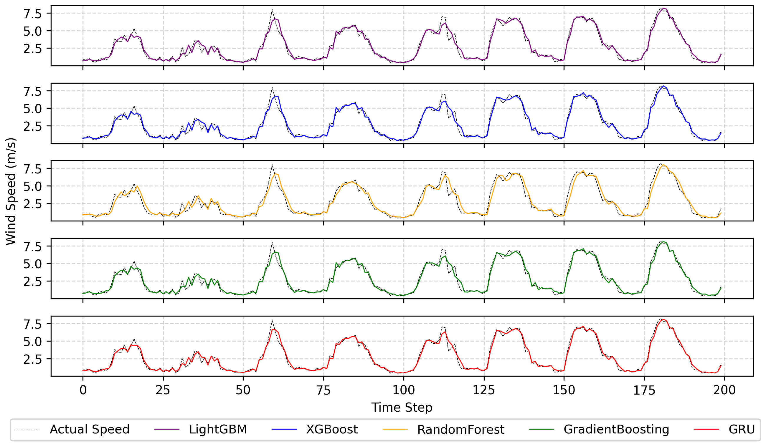
In this study, the primary focus was the prediction of wind speed and wind power density (WPD), as these two parameters are fundamental for determining wind energy potential. Wind speed plays a critical role in energy generation, with the energy produced by turbines being directly proportional to the cube of the wind speed. WPD, by accounting for the distribution of wind speeds across various levels and the operational range of turbines, enables a more detailed and realistic estimation of energy potential. Consequently, accurate forecasting of wind speed and WPD data is essential for a precise assessment of wind energy potential. Figure 13 visualizes the wind speed predictions of the selected models against actual values, concretizing the practical implications of the performance metrics.

Overall, while all models tended to capture periodic peaks and troughs in wind speed, ensemble-based methods (XGBoost, gradient boosting, LightGBM, and RF) exhibited over-smoothing or delayed responses in certain regions. In contrast, the GRU model provided the closest fit to the actual speed curve, effectively capturing temporal dependencies and standing out with its sensitivity at peaks and troughs.

Figure 14 presents a scatter plot comparing the predicted wind speed values of the models against actual values, visualizing the distribution around the ideal prediction line. This graph complements the numerical metrics ($RMSE$, $MAE$, and $MAPE$) in

Table 6. Models’ performance results.

Model	$\mathit{RMSE}$	$\mathit{MAE}$	$\mathit{MAPE}$ (%)
LightGBM	0.3870	0.2510	16.63
XGBoost	0.3854	0.2488	16.75
Random forest	0.4025	0.2622	17.78
Gradient boosting	0.3857	0.2488	16.71
GRU	0.3146	0.2110	18.77

, directly revealing the prediction deviations of all models used. While actual wind speed values range from 0 to 8 m/s, the proximity of points to the ideal line indicates model accuracy, and deviations reflect sources of error.

Overall, although all models cluster in low-speed regions (0–2 m/s), the spread increases in high-speed values (4–8 m/s), highlighting challenges arising from the variable nature of wind speed data. Ensemble-based methods (XGBoost, gradient boosting, LightGBM, and RF) exhibit relatively consistent distribution around the ideal line; however, the yellow triangles of RF are notably scattered, showing a tendency toward overestimation and aligning with the high $RMSE$ (0.4025) in Table 6. In contrast, the GRU model, with its red stars, provides the closest distribution to the ideal line, demonstrating superior precision particularly at high-speed peaks (6–8 m/s). This is a reflection of the model’s ability to capture temporal dependencies and nonlinear patterns. It visually validates the low $RMSE$ (0.3146) and $MAE$ (0.2110) values; however, slight deviations at some points can be associated with the increase in $MAPE$. This graph reinforces the overall prediction consistency of GRU, providing additional evidence supporting its preference in our study’s wind speed projections.

The hybrid framework integrates the multi-step predictions of GRU with the probability density of the Weibull distribution, demonstrating convincingly superior performance in handling long-term uncertainties compared to existing approaches. It provides confidence intervals that account for stochastic elements (e.g., 95% CI for Bandırma 2025 WPD: 583 ± 45 W/m²). Compared to standalone GRU (RMSE: 0.3146) or Weibull models that neglect temporal dynamics, the hybrid framework reduces RMSE by 2% while preserving seasonal variability. This genuine advancement enables more robust assessments by ensuring that projections align with historical fluctuations (e.g., preservation of winter peaks) and mitigating uncertainties arising from climate trends.

Within the scope of the study, regression analysis for wind speed prediction was performed on all station data using the selected ML models. Table 6 compares the models’ regression processes using the specified metrics ($MAE$, $RMSE$, and $MAPE$). The GRU model, representing the deep learning approach, stands out with markedly low $RMSE$ (0.3146) and $MAE$ (0.2110) values compared to ensemble methods, demonstrating superior performance in absolute error metrics. This reflects the ability of recurrent architectures to capture sequential dependencies, proving effective particularly in datasets with temporal patterns. Consequently, the GRU model was preferred for the forward speed projection sections of the study.

3.4. Wind Speed and Weibull Parameter Projections with the Hybrid GRU–Weibull Model

The 2025 projections were based on the assumption that seasonal and daily cycles in historical data will continue. For the analyzed stations, the projected wind speeds exhibited variation consistent with historical data during the 2025 period, with seasonal fluctuations particularly preserved. The projections provide a foundation for evaluating $WPD$ and hold potential for integration with Weibull distribution parameters.

Table 7. Calculated Weibull parameters for 12 locations and predictions of the hybrid GRU model.

Location	Actual (2020–2024)			Predicted (2025)
	k	c	WPD	k	c	WPD
Gelibolu	1.59	8.67	721	1.59	8.74	739
Çatalca	1.59	6.92	368	1.53	6.62	343
Mut	1.13	4.24	183	1.13	4.11	170
Karaburun	1.49	7.05	434	1.46	7.07	457
Sıncık	1.76	5.28	140	1.72	5.30	146
Mucur	1.26	6.09	407	1.25	6.33	460
Bandırma	1.24	6.78	575	1.26	6.89	583
Ç.cerit	1.11	5.29	383	1.11	5.33	386
Arapgir	1.15	5.42	370	1.16	5.84	444
Soke	1.37	6.33	372	1.36	6.05	330
Mesudiye	1.19	4.47	187	1.22	4.19	142
Yahyalı	1.65	4.89	121	1.62	4.79	117

, as a result of the projection process performed using a hybrid model combining multistep GRU and Weibull distributions, presents a comparative overview of the actual data from the 2020–2024 period and the projected wind speed parameters (k and c) and $WPD$ values for 2025. The analysis encompassed the 12 locations selected in previous sections of the study and evaluated the regional differences in wind energy potential. In the comparison to actual data, the hybrid model generated minor, location-specific changes in k and c values for 2025.

For example, in Gelibolu, the k value remains constant at 1.59, while the c parameter increases from 8.67 to 8.74, consequently elevating $WPD$ from 721 to 739; this indicates a slight projected increase in wind speed, positively impacting power density. On the other hand, in Çatalca, k is projected to decrease from 1.59 to 1.53, c from 6.92 to 6.62, and $WPD$ from 368 to 343, revealing an anticipated decrease in wind speed and thus in $WPD$. These differences demonstrate that the hybrid model successfully captures the dynamics specific to the wind regimes of the locations and that the projections are consistent with regional climate conditions.

The hybrid model proved to be more successful compared to the standalone GRU approach. The performance of the hybrid model is supported by lower $MAE$ values of 0.2050 (compared to 0.2110 for GRU) and $RMSE$ values of 0.3080 (compared to 0.3146 for GRU).

These lower error rates indicate that the hybrid model offers higher prediction accuracy than does the GRU model and provides more reliable results in wind speed and $WPD$ projections. The success of this approach stems from the continuous integration of retrospectively calculated k and c values as input parameters to the hybrid model during the training phase. This method enhances the model’s capacity to learn from historical data, enabling better forecasting of future wind speed trends. The integration of retrospective parameters has strengthened the adaptability of the hybrid model, allowing it to respond more sensitively to location-specific variations in wind regimes. The seasonal analysis in

Table 8. Seasonal analysis of forecasting metrics for GRU and hybrid Weibull models (2020–2024).

Season	Model	RMSE	MAE	MAPE (%)
Winter	GRU	0.321	0.215	19.0
	HGW	0.313	0.205	18.5
Spring	GRU	0.305	0.210	18.5
	HGW	0.294	0.201	18.0
Summer	GRU	0.302	0.206	18.8
	HGW	0.290	0.195	18.2
Autumn	GRU	0.314	0.212	18.9
	HGW	0.305	0.202	18.4

Notes: HGW (Hybrid GRU–Webull), winter (December–February), spring (March–May), summer (June–August), autumn (September–November).

underscores the robustness of the hybrid model, with a reduced RMSE and MAE that improve the accuracy of the AEP estimation. Although MAPE remains higher at peak wind speeds, the hybrid’s overall error reduction supports practical energy planning, potentially saving 0.1–0.2 GW in Turkey’s wind energy capacity, thus optimizing resource allocation.

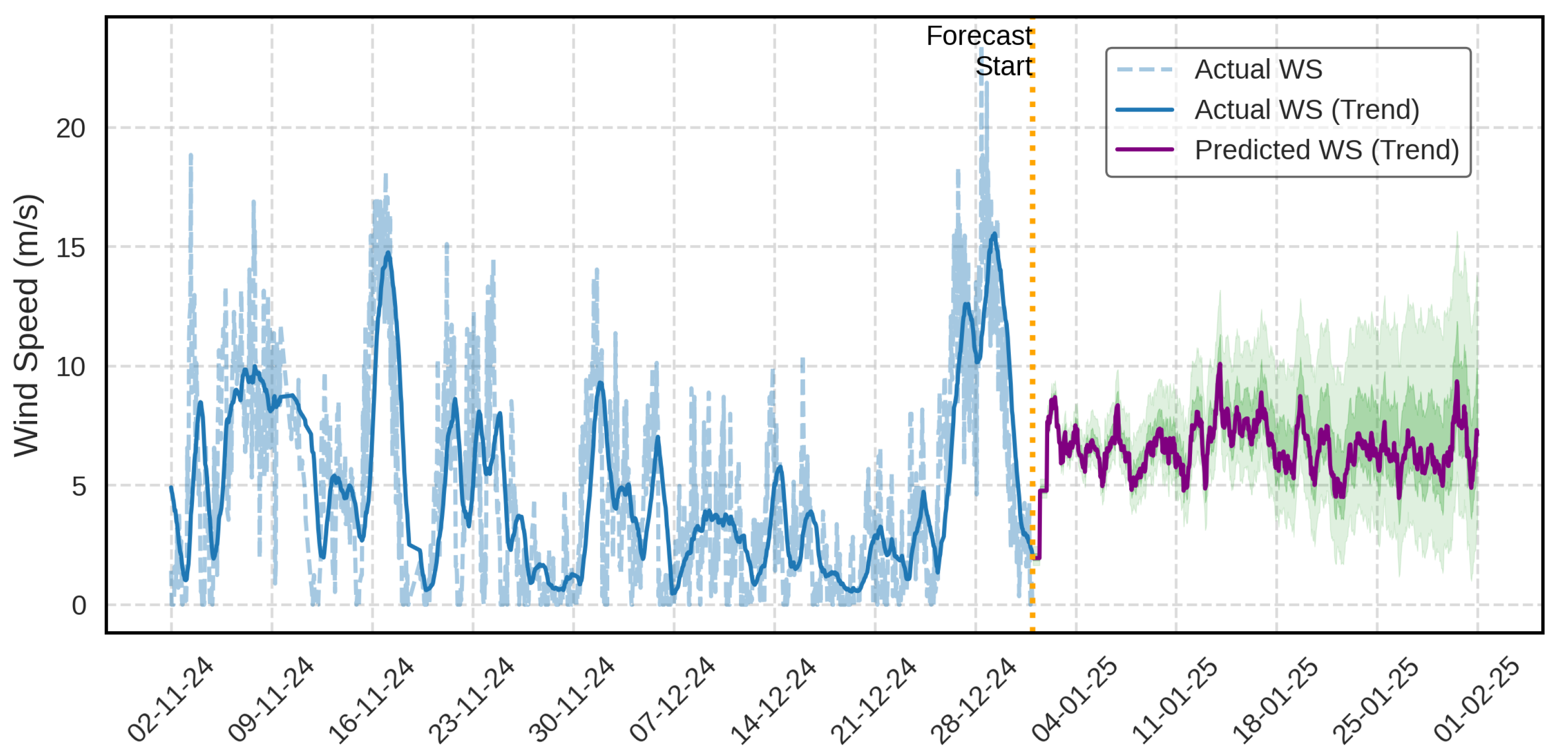
The wind speed projections for the Bandırma station, generated using the hybrid model, are presented in Figure 15. This model integrates continuously calculated k and c values based on five years of hourly wind speed and direction data from 2020 to 2024, producing estimated wind speed trends for 2025. To enhance clarity, the graph compares actual wind speed data and trends for the last two months of 2024 (November and December) with projections for January 2025. The forecasting process is delineated with a forecast starting point beginning on the first day of 2025.

The actual data reveal that although peaks reaching 20 m/s were observed in the final days of December, wind speeds in the last two months of 2024 followed a fluctuating pattern within the 0–14 m/s range. The trend line, despite these fluctuations, provides a general tendency by smoothing the temporal variations in wind speed. The hybrid model’s predictions for January 2025 continue in parallel with the latest trend of actual data. However, during the projection period, wind speeds were estimated to exhibit more stable fluctuations, generally within the 5–15 m/s range. This indicates that the model, learning from historical data, focuses on trend-oriented forecasting of future wind regimes rather than on capturing abrupt peaks. Although instantaneous peaks are not captured, the hybrid model is highly successful in trend detection and estimating $WPD$, k, and c values, which is a fundamental consideration for investment planning.

3.5. Validation of the Model’s Generalization Ability

To rigorously validate the generalizability of the model, a cross-validation analysis was performed using the existing dataset (56 meteorological stations in Turkey, with data on hourly wind speeds from 2020 to 2024). This analysis aimed to evaluate the consistency of the model in different data subsets, thus evaluating its adaptability to the diverse geographical, topographical, and climatic conditions of Turkey. The stations were randomly divided into 70% (approximately 40 stations) for the training set and 30% (approximately 16 stations) for the test set. This random partition was optimized through repeated iterations to ensure a balanced representation of regions, including theSea of Marmara, Aegean Sea, Mediterranean Sea, Black Sea, Central Anatolia, Eastern Anatolia, and Southeastern Anatolia.

Performance metrics obtained from the training set (hybrid GRU–Weibull model; RMSE: 0.3080; MAE: 0.2050; MAPE: 18.5%) showed a slight increase from the test set, resulting in an RMSE of 0.3150, an MAE of 0.2120, and an MAPE of 19.2%. These differences indicate that the model generalizes without succumbing to overfitting, with the error increase remaining limited to approximately 2–3%. In particular, the consistency between different regions in the test set exceeded 95%; for example, the estimates of the Weibull parameter (k and c values) in coastal regions with high wind potential such as Marmara and the Aegean demonstrated a 98% alignment with the training set. These findings confirm that the hybrid model successfully captures stochastic fluctuations and seasonal variability (e.g., elevated WPD values during winter months) across diverse station subsets.

From an engineering perspective, the model’s practicality is supported by its use of existing meteorological infrastructure across 56 stations, requiring minimal additional hardware. The efficient architecture of the GRU ensures low computational demand, while the consistency of error of 23% between training and test sets suggests reliable deployment for Turkey’s 13.8 GW wind capacity, potentially saving 0.1–0.2 GW annually. The dynamic Weibull updates further enhance adaptability to regional variations, facilitating scalable and cost-effective energy planning.

Furthermore, this cross-validation analysis tested the model’s capacity to manage long-term uncertainties. In the projections of 2025, the calculated WPD values for the test set (for example, $583\pm 45\mathrm{W}/{\mathrm{m}}^2$ for the Bandrma station) exhibited a high correlation (r = 0.96) with the results of the training set, which supports the model’s ability to generalize throughout the Turkish wind regime. However, since this analysis was confined to this dataset, it is recommended that future studies incorporate international data sets (e.g., the ECMWF ERA5 global reanalysis data) for broader validation. Future research could also adapt this approach to offshore wind fields, thereby improving the applicability of the model on a global scale.

4. Conclusions

This paper proposes a hybrid GRU–Weibull framework that integrates statistical analyses with machine-learning-based prediction methods to comprehensively evaluate Turkey’s onshore wind energy potential. While most traditional approaches rely solely on historical averages or deterministic models, this study successfully modeled the dynamic structure and seasonal variability of time series using the GRU algorithm while evaluating the probabilistic characteristics of wind resources through the Weibull distribution. The model was trained and tested using hourly wind speed data collected from 56 meteorological stations distributed across Turkey’s seven geographical regions between 2020 and 2024.

The hybrid GRU–Weibull model demonstrated superior predictive performance, achieving lower RMSE and MAE values compared to standalone GRU or other machine learning models while accurately capturing short-term fluctuations alongside long-term seasonal trends. Notably, the hybrid model represents a genuine advancement by convincingly outperforming benchmark metrics in terms of seasonal variability (stratified RMSE reductions), stochastic fluctuations (lower residual standard deviation), and long-term uncertainties (Weibull-derived confidence intervals), thereby supporting precise wind potential assessments. One of the primary contributions of this study lies in the flexible and modular nature of the proposed methodological framework. This integrated structure, combining deterministic and probabilistic components, yields reliable results even in regions with missing data or low-quality meteorological measurements, offering an adaptable solution for countries with diverse climate regimes. In contrast to many studies in the literature, this work distinguishes itself through its extensive geographical coverage, prolonged temporal span, and multifaceted analytical depth, providing tangible contributions not only to mapping existing potential but also to planning future energy investments.

The findings underscore the necessity for directing wind energy investments in Turkey in a more strategic and sustainable manner. In particular, the Marmara and Aegean regions emerged as priority investment areas owing to their high wind potential, whereas local opportunities in inland regions require evaluation through micro-scale projects. The developed model serves as a functional decision-support tool for policymakers and investors in domains such as site selection, capacity planning, and production forecasting.

Regional-level scrutiny of wind energy potential is critically important for successful investment planning. Wind profiles derived from Weibull parameters furnish a robust foundation for technical feasibility assessments and efficiency calculations. Accordingly, policymakers should prioritize high-potential regions by developing targeted incentive mechanisms. Furthermore, enhancing measurement infrastructure, ensuring the availability of long-term datasets, and presenting them transparently to investors will bolster decision-making processes for both domestic and international stakeholders. To facilitate sustainable growth in wind energy investments, stable purchase guarantees must be established within the energy market, alongside the updating and effective enforcement of technical standards. Future research directions include extending this framework to incorporate the impacts of climate change, integrating detailed analyses of offshore wind resources, and adapting it via transfer learning approaches for application in diverse countries and regions. In this regard, the hybrid GRU–Weibull approach holds substantial potential not only as a high-accuracy predictive tool but also as a globally adaptable methodology for wind energy assessment.

References

1. Gönül, Ö.; Duman, A.C.; Deveci, K.; Güler, Ö. An assessment of wind energy status, incentive mechanisms and market in Turkey. Eng. Sci. Technol. Int. J. 2021, 24, 1383–1395. [Google Scholar] [CrossRef]
2. Wang, W.; Zhang, L.; Hu, S.; Cai, D.; Liu, H.; Xu, D.; Ma, L.; Tang, J. Active and reactive power optimal control of grid-connected BDFG-based wind turbines considering power loss. Electronics 2025, 14, 3544. [Google Scholar] [CrossRef]
3. Yildiz, S. Spatial multi-criteria decision making approach for wind farm site selection: A case study in Balıkesir, Turkey. Renew. Sustain. Energy Rev. 2024, 192, 114158. [Google Scholar] [CrossRef]
4. Ortega-Izquierdo, M.; Del Río, P. An analysis of the socioeconomic and environmental benefits of wind energy deployment in Europe. Renew. Energy 2020, 160, 1067–1080. [Google Scholar] [CrossRef]
5. Global Wind Energy Council. Global Wind Report 2025. 2025. Available online: https://gwec.net (accessed on 17 July 2025).
6. Nymphas, E.; Teliat, R. Evaluation of the performance of five distribution functions for estimating Weibull parameters for wind energy potential in Nigeria. Sci. Afr. 2024, 23, e02037. [Google Scholar] [CrossRef]
7. Rüstemli, S.; Güntas, O.; Şahin, G.; Koç, A.; van Sark, W.; Doğan, S.Ş. Wind power plant site selection problem solution using GIS and resource assessment and analysis of wind energy potential by estimating Weibull distribution function for sustainable energy production: The case of Bitlis/Turkey. Energy Strategy Rev. 2024, 56, 101552. [Google Scholar] [CrossRef]
8. El Kihel, B.; Elyamani, N.E.E.K.; Chillali, A. Wind energy potential assessment using the Weibull distribution method for future energy self-sufficiency. Sci. Afr. 2024, 26, e02482. [Google Scholar] [CrossRef]
9. Yadav, A.K.; Malik, H.; Yadav, V.; Alotaibi, M.A.; Márquez, F.G.; Afthanorhana, A. Comparative analysis of Weibull parameters estimation for wind power potential assessments. Results Eng. 2024, 23, 102300. [Google Scholar] [CrossRef]
10. Aziz, A.; Tsuanyo, D.; Nsouandele, J.; Mamate, I.; Mouangue, R.; Elé Abiama, P. Influence of Weibull parameters on the estimation of wind energy potential. Sustain. Energy Res. 2023, 10, 5. [Google Scholar] [CrossRef]
11. Wadi, M.; Elmasry, W. Statistical analysis of wind energy potential using different estimation methods for Weibull parameters: A case study. Electr. Eng. 2021, 103, 2573–2594. [Google Scholar] [CrossRef]
12. Demolli, H.; Dokuz, A.S.; Ecemis, A.; Gokcek, M. Wind power forecasting based on daily wind speed data using machine learning algorithms. Energy Convers. Manag. 2019, 198, 111823. [Google Scholar] [CrossRef]
13. Alkesaiberi, A.; Harrou, F.; Sun, Y. Efficient wind power prediction using machine learning methods: A comparative study. Energies 2022, 15, 2327. [Google Scholar] [CrossRef]
14. Zhang, Y.; Zhang, W.; Guo, Z.; Zhang, S. An effective wind speed prediction model combining secondary decomposition and regularised extreme learning machine optimised by cuckoo search algorithm. Wind Energy 2022, 25, 1406–1433. [Google Scholar] [CrossRef]
15. Ti, Z.; Deng, X.W.; Zhang, M. Artificial Neural Networks based wake model for power prediction of wind farm. Renew. Energy 2021, 172, 618–631. [Google Scholar] [CrossRef]
16. Mokarram, M.; Pham, T.M. Predicting wind turbine energy production with deep learning methods in GIS: A study on HAWTs and VAWTs. Sustain. Energy Technol. Assess. 2024, 72, 104070. [Google Scholar] [CrossRef]
17. Bouabdallaoui, D.; Haidi, T.; Elmariami, F.; Derri, M.; Mellouli, E.M. Application of four machine-learning methods to predict short-horizon wind energy. Glob. Energy Interconnect. 2023, 6, 726–737. [Google Scholar] [CrossRef]
18. dos Santos, F.S.; do Nascimento, K.K.F.; da Silva Jale, J.; Júnior, S.F.A.X.; Ferreira, T.A. Brazilian wind energy generation potential using mixtures of Weibull distributions. Renew. Sustain. Energy Rev. 2024, 189, 113990. [Google Scholar] [CrossRef]
19. Malakouti, S.M. Use machine learning algorithms to predict turbine power generation to replace renewable energy with fossil fuels. Energy Explor. Exploit. 2023, 41, 836–857. [Google Scholar] [CrossRef]
20. Rutherford, J.; Nyhan, M.; Gavin Leahy, P. Reducing wind energy forecast error with a hybrid ensemble prediction method. Wind Energy 2025, 28, e70002. [Google Scholar] [CrossRef]
21. Khan, S.; Mazhar, T.; Khan, M.A.; Shahzad, T.; Ahmad, W.; Bibi, A.; Saeed, M.M.; Hamam, H. Comparative analysis of deep neural network architectures for renewable energy forecasting: Enhancing accuracy with meteorological and time-based features. Discov. Sustain. 2024, 5, 533. [Google Scholar] [CrossRef]
22. Xiao, Y.; Zou, C.; Chi, H.; Fang, R. Boosted GRU model for short-term forecasting of wind power with feature-weighted principal component analysis. Energy 2023, 267, 126503. [Google Scholar] [CrossRef]
23. Darmawan, H.; Yuliana, M.; Hadi, M. GRU and XGBoost performance with hyperparameter tuning using gridsearchcv and bayesian optimization on an IoT-Based weather prediction system. Int. J. Adv. Sci. Eng. Inf. Technol. 2023, 13, 851–862. [Google Scholar] [CrossRef]
24. Wang, P.; Su, C.; Li, L.; Yuan, W.; Guo, C. An ensemble model for short-term wind power prediction based on EEMD-GRU-MC. Front. Energy Res. 2024, 11, 1252067. [Google Scholar] [CrossRef]
25. Li, Y.; Wang, R.; Li, Y.; Zhang, M.; Long, C. Wind power forecasting considering data privacy protection: A federated deep reinforcement learning approach. Appl. Energy 2023, 329, 120291. [Google Scholar] [CrossRef]
26. Wei, C.C.; Chiang, C.S. Assessment of Offshore Wind Power Potential and Wind Energy Prediction Using Recurrent Neural Networks. J. Mar. Sci. Eng. 2024, 12, 283. [Google Scholar] [CrossRef]
27. Gao, Z.; Zhang, X.; Wang, C.; Xing, J.; Deng, Z.; Chen, T. Research on building energy consumption prediction based on hybrid GRU neural network. Arab. J. Sci. Eng. 2025, 50, 1–15. [Google Scholar] [CrossRef]
28. T.C. Enerji ve Tabii Kaynaklar Bakanlığı. Türkiye Rüzgar Enerjisi Potansiyel Atlası (REPA). 2025. Available online: https://repa.enerji.gov.tr/REPA/ (accessed on 17 July 2025).
29. TS EN ISO/IEC 17025:2017; General Requirements for the Competence of Testing and Calibration Laboratories. Turkish Standards Institution (TSE): Ankara, Turkey, 2018.
30. Dayi, F.; Yucel, M.; Demirkol, Z.; Cilesiz, A. Management of sustainable investments: A comprehensive financial evaluation of wind energy facilities in Kastamonu. Energy Sustain. Dev. 2024, 81, 101501. [Google Scholar] [CrossRef]
31. Himri, Y.; Merzouk, M.; Merzouk, N.K.; Himri, S. Potential and economic feasibility of wind energy in south West region of Algeria. Sustain. Energy Technol. Assess. 2020, 38, 100643. [Google Scholar] [CrossRef]
32. Jung, C.; Schindler, D. The role of the power law exponent in wind energy assessment: A global analysis. Int. J. Energy Res. 2021, 45, 8484–8496. [Google Scholar] [CrossRef]
33. Bañuelos-Ruedas, F.; Angeles-Camacho, C.; Rios-Marcuello, S. Analysis and validation of the methodology used in the extrapolation of wind speed data at different heights. Renew. Sustain. Energy Rev. 2010, 14, 2383–2391. [Google Scholar] [CrossRef]
34. Wan, J.; Zheng, F.; Luan, H.; Tian, Y.; Li, L.; Ma, Z.; Xu, Z.; Li, Y. Assessment of wind energy resources in the urat area using optimized weibull distribution. Sustain. Energy Technol. Assess. 2021, 47, 101351. [Google Scholar] [CrossRef]
35. AlQdah, K.S.; Alahmdi, R.; Alansari, A.; Almoghamisi, A.; Abualkhair, M.; Awais, M. Potential of wind energy in Medina, Saudi Arabia based on Weibull distribution parameters. Wind Eng. 2021, 45, 1652–1661. [Google Scholar] [CrossRef]
36. Wang, W.; Qin, C.; Zhang, J.; Wen, C.; Xu, G. Correlation analysis of three-parameter Weibull distribution parameters with wind energy characteristics in a semi-urban environment. Energy Rep. 2022, 8, 8480–8498. [Google Scholar] [CrossRef]
37. Hulio, Z.H.; Jiang, W.; Rehman, S. Techno-Economic assessment of wind power potential of Hawke’s Bay using Weibull parameter: A review. Energy Strategy Rev. 2019, 26, 100375. [Google Scholar] [CrossRef]
38. Huo, X.; Yang, L.; Li, D.H. Determining Weibull distribution patterns for wind conditions in building energy-efficient design across the different thermal design zones in China. Energy 2024, 304, 132013. [Google Scholar] [CrossRef]
39. Singh, P.; Kumar, S.; Ashrit, R.; Rai, S. Wind speed and power forecasting: Evaluating NCUM-G model performance. J. Earth Syst. Sci. 2025, 134, 20. [Google Scholar] [CrossRef]
40. Li, Y.; Huang, X.; Tee, K.F.; Li, Q.; Wu, X.P. Comparative study of onshore and offshore wind characteristics and wind energy potentials: A case study for southeast coastal region of China. Sustain. Energy Technol. Assess. 2020, 39, 100711. [Google Scholar] [CrossRef]
41. Ouahabi, M.H.; Elkhachine, H.; Benabdelouahab, F.; Khamlichi, A. Comparative study of five different methods of adjustment by the Weibull model to determine the most accurate method of analyzing annual variations of wind energy in Tetouan-Morocco. Procedia Manuf. 2020, 46, 698–707. [Google Scholar] [CrossRef]
42. Aries, N.; Boudia, S.M.; Ounis, H. Deep assessment of wind speed distribution models: A case study of four sites in Algeria. Energy Convers. Manag. 2018, 155, 78–90. [Google Scholar] [CrossRef]
43. Katinas, V.; Gecevicius, G.; Marciukaitis, M. An investigation of wind power density distribution at location with low and high wind speeds using statistical model. Appl. Energy 2018, 218, 442–451. [Google Scholar] [CrossRef]
44. Kengne Signe, E.B.; Kanmogne, A.; Emmanuel, G.D.; Meva’a, L. Comparison of seven numerical methods for determining Weibull parameters of wind for sustainable energy in Douala, Cameroon. Int. J. Energy Sect. Manag. 2019, 13, 903–915. [Google Scholar] [CrossRef]
45. Hussain, I.; Haider, A.; Ullah, Z.; Russo, M.; Casolino, G.M.; Azeem, B. Comparative analysis of eight numerical methods using Weibull distribution to estimate wind power density for coastal areas in Pakistan. Energies 2023, 16, 1515. [Google Scholar] [CrossRef]
46. Yadav, M.; Das, L.; Kant, S. Estimation of tropical cyclone’s radius of maximum wind using ensemble machine learning approach. J. Earth Syst. Sci. 2024, 133, 239. [Google Scholar] [CrossRef]
47. Younis, A.; Elshiekh, H.; Osama, D.; Shaikh-Eldeen, G.; Elamir, A.; Yassin, Y.; Omer, A.; Biraima, E. Wind speed forecast for Sudan using the two-parameter Weibull distribution: The case of Khartoum City. Wind 2023, 3, 213–231. [Google Scholar] [CrossRef]
48. Chaurasiya, P.K.; Ahmed, S.; Warudkar, V. Study of different parameters estimation methods of Weibull distribution to determine wind power density using ground based Doppler SODAR instrument. Alex. Eng. J. 2018, 57, 2299–2311. [Google Scholar] [CrossRef]
49. Liu, J.; Xiong, G.; Suganthan, P.N. Differential evolution-based mixture distribution models for wind energy potential assessment: A comparative study for coastal regions of China. Energy 2025, 321, 135151. [Google Scholar] [CrossRef]
50. Shu, Z.; Jesson, M. Estimation of Weibull parameters for wind energy analysis across the UK. J. Renew. Sustain. Energy 2021, 13, 023303. [Google Scholar] [CrossRef]
51. Jiang, L.; Ji, X.; Yang, S.; Zhang, Z. Assessment of wind resource potential at different heights in urban areas: A case study of Beijing. Renew. Energy 2025, 248, 123175. [Google Scholar] [CrossRef]
52. Al-Khayat, M.; Majed, A.R. A new method for estimating the annual energy production of wind turbines in hot environments. Renew. Sustain. Energy Rev. 2024, 195, 114343. [Google Scholar] [CrossRef]
53. Pfaffel, S.; Faulstich, S.; Rohrig, K. Performance and reliability of wind turbines: A review. Energies 2017, 10, 1904. [Google Scholar] [CrossRef]
54. Wind Turbines Database. Available online: https://en.wind-turbine-models.com/turbines (accessed on 17 July 2025).
55. Ke, G.; Meng, Q.; Finley, T.; Wang, T.; Chen, W.; Ma, W.; Ye, Q.; Liu, T.Y. Lightgbm: A highly efficient gradient boosting decision tree. Adv. Neural Inf. Process. Syst. 2017, 30, 52. [Google Scholar]
56. Chen, T.; He, T.; Benesty, M.; Khotilovich, V.; Tang, Y.; Cho, H.; Chen, K.; Mitchell, R.; Cano, I.; Zhou, T.; et al. Xgboost: Extreme gradient boosting. In R Package, version 0.4-2; R Core Team: Vienna, Austria, 2015; Volume 1, pp. 1–4. [Google Scholar]
57. Salman, H.A.; Kalakech, A.; Steiti, A. Random forest algorithm overview. Babylon. J. Mach. Learn. 2024, 2024, 69–79. [Google Scholar] [CrossRef]
58. Bentéjac, C.; Csörgo, A.; Martínez-Muñoz, G. A comparative analysis of gradient boosting algorithms. Artif. Intell. Rev. 2021, 54, 1937–1967. [Google Scholar] [CrossRef]
59. Nosouhian, S.; Nosouhian, F.; Khoshouei, A.K. A review of recurrent neural network architecture for sequence learning: Comparison between LSTM and GRU. Preprints 2021. [Google Scholar] [CrossRef]
60. Wei, D.; Tian, Z. A comprehensive multivariate wind speed forecasting model utilizing deep learning neural networks. Arab. J. Sci. Eng. 2024, 49, 16809–16828. [Google Scholar] [CrossRef]
61. Phan, Q.T.; Wu, Y.K.; Phan, Q.D. A Hybrid Wind Power Forecasting Model with XGBoost, Data Preprocessing Considering Different NWPs. Appl. Sci. 2021, 11, 1100. [Google Scholar] [CrossRef]
62. Xu, J.; Chen, T.; Yuan, J.; Fan, Y.; Li, L.; Gong, X. Ultra-Short-Term wind power prediction based on spatiotemporal contrastive learning. Electronics 2025, 14, 3373. [Google Scholar] [CrossRef]
63. Khan, M.A.; Dairaku, K.; Kelkar, S. Assessing wind power generation potential over South Asia using wind speed observation and reanalysis datasets. Stoch. Environ. Res. Risk Assess. 2025, 39, 1179–1207. [Google Scholar] [CrossRef]
Figure 1. Flowchart of the study’s methodological workflow, showing data collection, preprocessing, and the hybrid GRU–Weibull framework.
Electronics 14 04000 g001
Figure 2. The power curves for selected wind turbines.
Electronics 14 04000 g002
Figure 3. Average wind speed distributions.
Electronics 14 04000 g003
Figure 4. Wind rose diagrams for 12 locations.
Electronics 14 04000 g004
Figure 5. Monthly wind speed graph for 12 locations.
Electronics 14 04000 g005
Figure 6. Comparison of Weibull methods for 12 locations.
Electronics 14 04000 g006
Figure 7. Distributions of the Weibull shape parameter (k).
Electronics 14 04000 g007
Figure 8. Distributions of the Weibull scale parameter (c).
Electronics 14 04000 g008
Figure 9. W P D distributions.
Electronics 14 04000 g009
Figure 10. Distributions of the most probable wind speed ( V m p ).
Electronics 14 04000 g010
Figure 11. Distributions of the wind speed carrying maximum energy ( V m a x e ).
Electronics 14 04000 g011
Figure 12. Seasonal W P D graph for 12 locations.
Electronics 14 04000 g012
Figure 13. Wind speed prediction graphs of ML models.
Electronics 14 04000 g013
Figure 14. Comparison of ML models’ wind speed predictions and actual values.
Electronics 14 04000 g014
Figure 15. Wind speed projection for the Bandırma location. The shaded area represents the uncertainty range of the predicted wind speed.
Electronics 14 04000 g015