Regression Analysis for Predicting the Magnetic Field Shielding Effectiveness of Ferrite Sheets

Abstract

In this paper, a method to predict near-field magnetic shielding effectiveness (NSE) of ferrite sheets is proposed by measuring their relative permeability. The NSE prediction for ferrite sheets is developed using eight regression models based on higher-order terms of permeability, extracted through Minitab’s regression analysis using data from the measured NSE and relative permeabilities of the ferrite sheets. To analyze the accuracy of the predicted NSE in comparison to the measured NSE, the mean square error (MSE) was computed. As a result, the extracted regression models enable fast and accurate NSE predictions for ferrite sheets up to 100 MHz, achieving an MSE of less than 1.0, in contrast to numerical simulation methods that require several hours.

1. Introduction

In modern electronic devices, high clock speeds, densely packed PCB layouts, and the proximity of high-speed circuits exacerbate electromagnetic interference (EMI) issues. Furthermore, the extensive use of wireless communication and sophisticated power management systems adds to the challenge. As concerns about EMI grow, the importance of effective shielding and noise suppression techniques is also increasing.

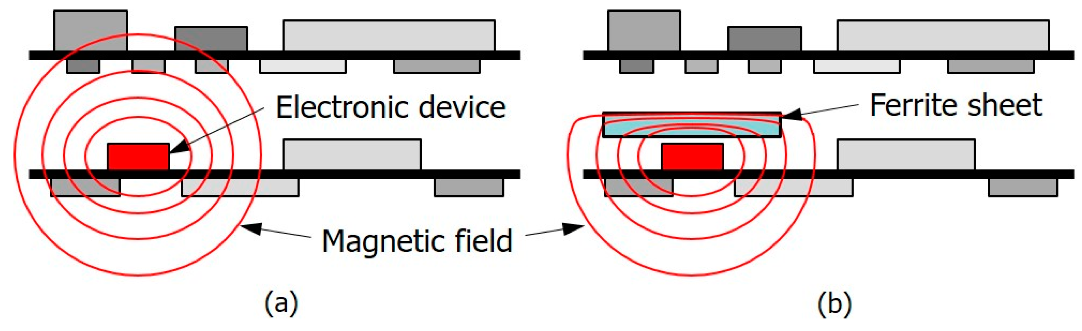
Magnetic sheets, typically made from flexible magnetic materials like ferrite or metal alloy composites, are designed to absorb and dissipate unwanted electromagnetic noise that can interfere with electronic circuits and components as shown in Figure 1. Furthermore, when the coupling between noisy components and susceptible components increases due to the metallic boxes or enclosures that package them, attaching magnetic sheets to the metallic surfaces can help reduce noise coupling caused by the induced currents on the inner conducting plane, as depicted in Figure 2. Therefore, in an increasingly noisy electromagnetic environment, magnetic sheets are indispensable for maintaining the performance and integrity of electronic devices.

In particular, noise suppression sheets (NSSs) are commonly employed for reducing and suppressing noise coupling and propagation at the GHz frequency range in modern electronic devices. Numerous studies have been conducted on NSSs [1,2,3,4,5]. In addition to their use in the GHz high-frequency range, magnetic sheets are increasingly being employed to reduce low-frequency noise in electric vehicles [6,7]. The noise reduction mechanisms of magnetic sheets differ between high-frequency and low-frequency ranges. In high-frequency ranges, noise is absorbed due to the loss characteristics associated with the imaginary component of the permeability of the magnetic material. In contrast, in low-frequency ranges, the real component of the permeability causes the magnetic field to concentrate within the magnetic material, thereby converting or guiding the magnetic field path to reduce noise coupling between the noise source and victim circuits.

During the design phase of electronic devices, accurately predicting the near-field magnetic shielding properties of magnetic sheets is essential for selecting the most suitable materials to mitigate noise coupling. However, conventional approaches that rely on numerical simulations, such as finite element analysis (FEA) or other complex computational methods, have several limitations. These simulations often demand computational time and resources due to the complexity of the magnetic materials and the need to model intricate device geometries accurately. Additionally, they require specialized expertise to set up and interpret the results effectively, making the process labor-intensive and potentially impractical for quick design iterations. As a result, there is a need for more efficient prediction methods that can provide reliable results with less effort and time investment.

In this paper, we propose a method to predict the near-field magnetic shielding effectiveness (NSE) of the ferrite-based magnetic materials up to 100 MHz by measuring their real permeability using regression analysis. To extract the eight regression models, complex relative permeability and NSE were measured using commercial ferrite sheets. Additionally, the differences or errors between the predicted NSE from the extracted regression models and the measured NSE were analyzed using an error assessment indicator: mean square error (MSE). The results confirmed that the proposed regression models provide sufficiently accurate predictions of NSE in the low-frequency range up to 100 MHz. The proposed method achieves comparable accuracy with negligible computational time when compared to numerical simulations.

2. Methodology

The procedure of regression analysis consists of three phases for predicting the NSE of ferrite sheets and for verifying the accuracy of the predicted results, as illustrated in Figure 3. In phase 1, regression models were developed using the measured permeability and NSE data of five commercial ferrite sheets (Group #1). The regression analysis was performed using Minitab [8]. In phase 2, the NSE was predicted using the measured permeability data of another two commercial ferrite sheets (Group #2) as input for the extracted regression models. In phase 3, the NSE of the ferrite sheets in Group #2 was measured, and the accuracy was verified by comparing them with the predicted NSE. The predicted NSE of the ferrite sheets in Group #1 used for extracting the regression models was also compared with the measured NSE.

The prediction of NSE is made by the regression models, which were extracted through the measured frequency-dependent permeabilities and the NSE of five commercial ferrite sheets (Group #1). For NSE prediction, the measured permeability is required not only for the ferrite sheet in Group #1 but also for the ferrite sheets in Group #2. The complex relative permeability of the ferrite sheets was measured from 1 kHz to 100 MHz using the 16454A magnetic material test fixture provided by Keysight [9]. A material under test (MUT) with a toroidal core shape and a thickness below 3 mm was coiled with a wire. Its relative permeability was calculated by measuring the impedance of the MUT based on the relationship between inductance and permeability.

Table 1. Real relative permeability at 1 MHz and thickness of ferrite sheets used in the analysis.

Name of MUTs		Real Relative Permeability at 1 MHz	Thickness 1
Group #1	R1	143	0.4
	R2	166	0.4
	R3	273	0.2
	R4	316	0.4
	R5	734	0.2
Group #2	P1	152	0.4
	P2	324	0.3

¹ The unit is mm.

lists the measured real relative permeability at 1 MHz and the thickness of the commercial ferrite sheets used in the analysis.

The NSE was measured using a microstrip line and loop probe [10,11,12]. Figure 4 shows a fabricated test fixture for magnetic shielding measurement of a thin magnetic sheet, which consists of a test board with a 50 $\mathsf{\Omega }$ microstrip line and a loop probe. The size of the test board is 140 mm $\times$ 140 mm and the thickness is 2.0 mm with FR4 substrate (${\epsilon }_r$ = 4.3). The length and width of the microstrip line are 60 mm and 3.78 mm, respectively. To capture the leakage near-field passing through a magnetic sheet, a magnetic loop probe (RF-R 400-1 [13]) with a diameter is 24 mm is employed. The distance (h) between the loop probe and microstrip line is set to be 1 mm. The size of ferrite sheets is 140 $\times$ 140 mm, which is the same as that of the test board and is sufficiently larger than that of the loop probe. The ferrite sheets are mounted at the center of the test board. One port of the vector network analyzer (VNA) is connected to the microstrip line, and the other port is connected to the loop probe. The other end of the microstrip line is terminated by 50 $\mathsf{\Omega }$. The NSE is defined by a ratio of two-port S-parameters between the microstrip line and loop probe as NSE $=20 {log}_{10}(S_{21}^R/S_{21}^L)$, where $S_{21}^R \mathrm{a}\mathrm{n}\mathrm{d} S_{21}^L$ are transmission coefficients of S-parameters in the absence (reference) and presence (load) of the magnetic sheet, respectively. The measured permeabilities and NSE were used as input data for Minitab’s regression analysis to obtain the regression models.

Figure 5 shows the complex relative permeability and near-field magnetic SE (NSE) of the R2 ferrite sheet with 0.4 mm thickness measured up to 100 MHz. The real part of the relative permeability remains nearly constant up to 10 MHz, peaks at 20 MHz, and then decreases linearly at higher frequencies. The imaginary part of the permeability is close to zero up to 10 MHz, increases up to approximately 30 MHz, and then decreases. The measured NSE closely follows the changes in the real permeability of the MUT as a function of frequency. This indicates that the NSE is determined by the value of the real permeability and can be predicted using the real permeability value.

Eight regression models were derived using the measured real relative permeability and NSE of five ferrite sheets in Group #1. Model #1 is a linear combination of frequency and real permeability. Model #2 adds a square term of the permeability to this linear combination and Model #3 includes up to a cubic term of the permeability. Model #4 includes the fourth-order term of permeability. Model #5 incorporates a square term of the frequency into the linear combination of frequency and real permeability, and Model #6 includes both the square terms of frequency and permeability. Model #7 includes the third-order term of permeability from Model #6, while Model #8 includes the fourth-order term of permeability from Model #7. All models contain a linear term of thickness. As a result, these models demonstrate the impact of higher-order terms of permeability and frequency on the prediction accuracy of NSE. These models are determined by the coefficients in front of each term, which are derived through Minitab’s regression analysis, and the results are listed in

Table 2. Extracted eight regression models, their adjusted coefficient of determination (R-Sq(adj)), and p-values in regression analysis.

Models	Prediction Equations of NSE *	R-Sq(adj)	p-Value
#1	$\mathrm{NSE}=9.03-0.0345\times f^{*}+23.2\times t^{*}+0.0209\times {\mu }_r$	89.2%	0.00
#2	$\mathrm{NSE}=4.31+0.00068\times f+25.2\times t+0.0451\times {\mu }_r-0.285\times {{{10}^{-4}\times (\mu }_r)}^2$	92.6%	0.00
#3	$\mathrm{NSE}=0.70+0.0234\times f+25.5\times t+0.08\times {\mu }_r-0.134\times {10}^{-3}\times {{(\mu }_r)}^2$                                                $-0.902\times {10}^{-7}\times {{(\mu }_r)}^3$	93.3%	0.00
#4	$\mathrm{NSE}=-3.14+0.042\times f+25.5\times t+0.135\times {\mu }_r-0.411\times {10}^{-3}\times {{(\mu }_r)}^2$                                 $+0.641\times {10}^{-6}\times {{(\mu }_r)}^3-0.364\times {10}^{-9}\times {{(\mu }_r)}^4$	93.9%	0.00
#5	$\mathrm{NSE}=7.49+0.05237\times f-0.0941\times {10}^{-2}\times f^2+24.3\times t+0.0227\times {\mu }_r$	91.7%	0.00
#6	$\mathrm{NSE}=2.74+0.0881\times f-0.0946\times {10}^{-2}\times f^2+26.3\times t+0.047\times {\mu }_r$                                                $-0.286\times {10}^{-4}\times {{(\mu }_r)}^2$	95.2%	0.00
#7	$\mathrm{NSE}=1.05+0.0926\times f-0.0872\times {10}^{-2}\times f^2+26.4\times t+0.0644\times {\mu }_r$                                $-0.818\times {10}^{-4}\times {{(\mu }_r)}^2+0.453\times {10}^{-7}\times {{(\mu }_r)}^3$	95.4%	0.00
#8	$\mathrm{NSE}=0.42+0.0926\times f-0.0834\times {10}^{-2}\times f^2+26.4\times t+0.0739\times {\mu }_{r }$                $-0.129\times {10}^{-3}\times {{(\mu }_r)}^2+0.136\times {10}^{-6}\times {{(\mu }_r)}^3-0.58\times {10}^{-10}\times {{(\mu }_r)}^4$	95.4%	0.00

* NSE is in dB, $f$ is in MHz, and $t$ is in mm.

.

When performing regression analysis, we should check two output results as criteria that determine the reliability of the analysis: p-value and adjusted coefficient of determination (R-Sq(adj)). The p-value measures the probability of obtaining the observed results, assuming that the null hypothesis is true. The lower the p-value, the greater the statistical significance of the observed difference. If insignificant independent variables are included in the regression equation, the R-Sq(adj) decreases and is often used as a criterion for selecting the optimal model. If the p-value is smaller than 0.05 and R-Sq(adj) is large, it means that the regression equation is statistically significant and accurate. 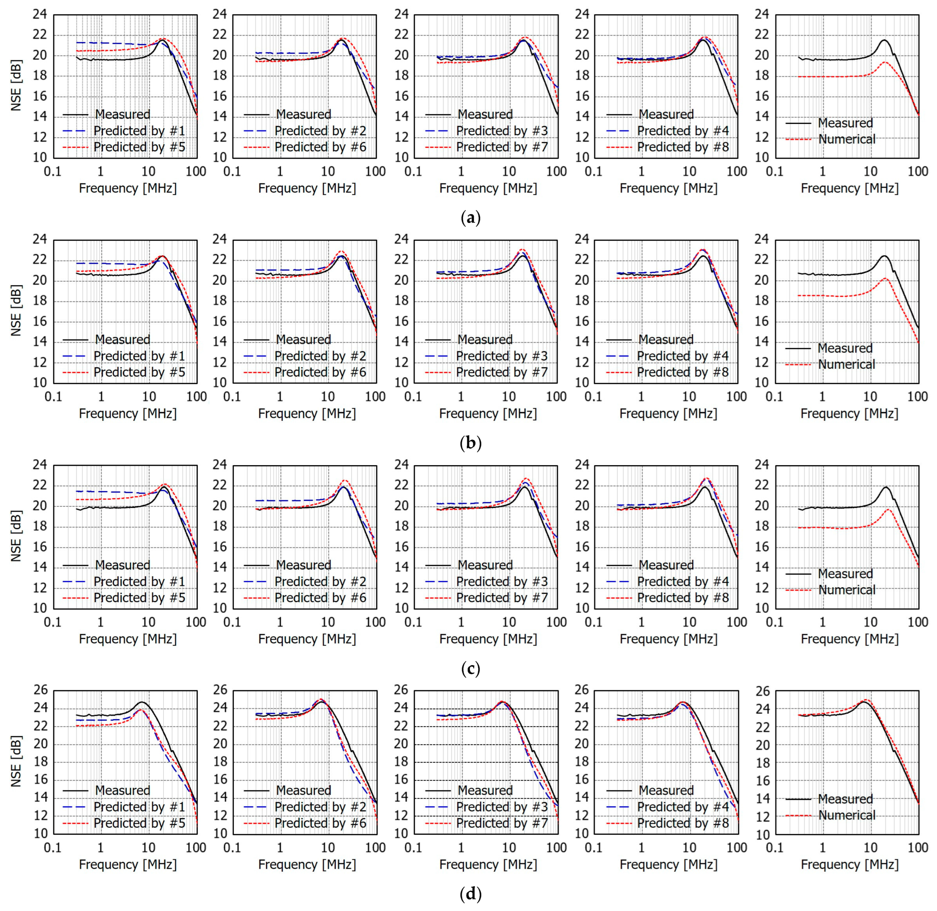Table 2 also lists the R-Sq(adj) and p-value for each model. It can be seen that the p-value for all models is 0.00, and the R-Sq(adj) for all models, except for Model #1, is above 90%, with R-Sq(adj) increasing to 95.4% in Models #7 and #8. This indicates that the extracted regression models are statistically significant and accurate. As higher-order terms of the permeability are included, the R-Sq(adj) increases, but models with the fourth-order term in permeability show similar R-Sq(adj) values to those with the third-order term. Therefore, it means that the fourth-order term of permeability is not necessary. Additionally, models that include the squared frequency term have a higher R-Sq(adj) compared to those that do not.

Figure 6 shows the regression analysis results for Model #6 and the residual plots for the predicted NSE. A normal probability plot of the residuals is used to check whether the residuals follow a normal distribution. The residuals histogram helps identify whether the data are skewed in a specific direction or if there are any outliers. The residuals versus fits plot is used to verify if the residuals are randomly distributed. If the plot shows a random distribution without any consistent pattern, it suggests that the assumptions of linearity and homoscedasticity are met. The residuals versus order plot checks whether the residuals are independent over time; if a specific pattern appears over time, it may indicate the presence of autocorrelation, suggesting that time-dependent factors are not accounted for in the regression model. Consequently, the residuals for the NSE in Model #6 are randomly distributed, follow a normal distribution, have no outliers, and are independent over time.

3. Comparison and Error Analysis

3.1. Comparison

The predicted NSE for the five ferrite sheets in Group #1 and the two ferrite sheets in Group #2 listed in Table 1 were calculated using the eight regression models. Figure 7 compares the predicted and measured NSE as a function of frequency for R1 and R2 in Group #1, and P1 and P2 in Group #2. As previously mentioned, the NSE characteristics up to 100 MHz can be broadly divided into three regions: a region where NSE remains constant below 10 MHz, a region around 20 MHz with a hill-like shape, and a region above 20 MHz where NSE decreases linearly. In the constant NSE region, all prediction models, except for Model #1, appear to show an error within 1 dB compared to the measured NSE. In the hill region around 20 MHz, prediction models other than Model #1 provide predictions that closely match the measured values. In the linearly decreasing region above 20 MHz, models with only the first-order frequency term (Model #1, #2, #3, and #4) appear to be more accurate than those including the second-order frequency term (Model #5, #6, #7, and #8). Anyway, the regression models provide predicted NSE that reasonably match the measured results for both the MUTs used in the model extraction and those not used in the extraction process. Consequently, various commercial magnetic sheets are verified and consistency is shown at the engineering level within 2 dB difference. It is confirmed that the proposed regression models can accurately predict the NSE of ferrite sheets using only the measured permeability values up to 100 MHz.

Additionally, the measured permeability was imported into CST Microwave Studio [14] to perform numerical simulations, and the results were compared with the measured NSE as shown in Figure 7. For R1, R2, and P1, the numerical simulation results were approximately 2 dB lower than the measured NSE values. In the case of P2, the numerical simulation results closely matched the measured values. Although it was challenging to pinpoint the exact cause of the discrepancies between the numerical and measured values, it was likely due to differences between the actual permeability of the magnetic sheets and the measured permeability, as well as discrepancies between the numerical simulation setup and the measurement conditions.

3.2. Error Analysis

To quantitatively analyze the difference or error between the predicted NSE and the measured NSE, the mean square error (MSE) was calculated [15] and compared. Figure 8 compares the accuracy of the eight regression models by calculating the MSE between the predicted and measured NSE for the five MUTs in Group #1 (for regression) and the two MUTs in Group #2 (for prediction) separately. As shown in Table 2, Models #1, #2, #3, and #4 include only the linear term for frequency, while Models #5, #6, #7, and #8 include the quadratic term for frequency as well. From Figure 8, it can be observed that models incorporating the quadratic term for frequency exhibit smaller MSE values. For models with only the linear term for frequency, the inclusion of higher-order permeability terms reduces the MSE. However, higher-order terms beyond the quadratic term do not significantly decrease the MSE. This trend also applies to models that include the quadratic term for frequency. In conclusion, the simplest predictive model with the smallest MSE is Model #6. For models with only the linear frequency term, the average MSE for Group #1 (Regression) and Group #2 (Prediction) fluctuates depending on the inclusion of higher-order permeability terms. However, for models incorporating the quadratic frequency term, the average MSE for Group #1 (Regression) is consistently smaller than that for Group #2 (Prediction). Model #6 achieves the smallest total average MSE across all MUTs.

Table 3. Comparison of averaged MSEs of extracted eight regression models and numerical simulation.

Models	Average Mean Square Errors (MSEs)
	Regression (Group #1)	Prediction (Group #2)	Total
#1	1.218	1.370	1.294
#2	0.833	0.761	0.797
#3	0.797	0.689	0.743
#4	0.643	0.760	0.702
#5	0.810	1.013	0.912
#6	0.435	0.484	0.460
#7	0.436	0.526	0.481
#8	0.426	0.556	0.491
Numerical	9.656	1.236	5.446

numerically presents the values shown in Figure 8. The values with the smallest MSE among the 8 models in each category (Regression, Prediction, and Total) have been bolded. Among the average MSEs of the MUTs in Group #1, which were used to extract the regression models, the smallest value is 0.426 for Model #8. For the MUTs in Group #2, which were used exclusively for prediction, the smallest average MSE is 0.484 for Model #6. The total average MSE for all models, except Model #1, is less than 1, with Model #6 having the smallest MSE of 0.46. In the case of numerical simulation, the average MSE for the MUTs in Group #1 is significantly higher, at 9.659, which is also evident in Figure 7. In contrast, the average MSE for the MUTs in Group #2 is 1.236. The total average MSE for numerical simulation is 5.446, which is ten times larger than that of Model #6. In conclusion, the prediction accuracy of the regression models is far superior to that of numerical simulation.

Lastly, the time required to calculate NSE using regression models was compared with the time required using numerical simulations. Here, the time to extract regression models was excluded; only the calculation time for NSE, given permeability data, was considered. For regression models, the calculations involve only basic arithmetic operations such as addition, subtraction, and multiplication, allowing results to be obtained almost instantaneously. In contrast, numerical simulations require extensive meshing due to the high permeability of the magnetic sheets. As a result, using a standard PC (Intel Core i7-6800K, 64 GB) without an accelerator, the simulation takes several hours to complete.

Table 4. Comparison of computation time.

Methods	Computation Time
Regression Models	<1 s
Numerical Simulation	>4 h 31 m 9 s

presents the NSE computation time for the smallest case among the seven sheets listed in Table 1. In conclusion, from a computation time perspective, regression models are significantly more efficient for NSE prediction compared to numerical simulation methods.

4. Conclusions

In this paper, we presented a method to predict the near-field magnetic shielding effectiveness (NSE) of ferrite sheets using the prediction models obtained through regression analysis. The commercial ferrite sheets used in the analysis were divided into Group #1 and Group #2. Eight regression models were developed using the measured relative permeability and NSE of the sheets in Group #1. The predicted NSE of the sheets in both Group #1 and Group #2 were then calculated and compared with the measured NSE. To verify the accuracy of the proposed regression models, an analysis of mean square errors (MSEs) was employed. The regression models with second-order frequency terms exhibited lower MSE compared to those with only first-order frequency terms. Additionally, while the inclusion of higher-order permeability terms further reduced MSE, the improvement was not significant beyond quadratic terms. Among the eight regression models, Model #6, which includes quadratic terms for both frequency and permeability, achieved the smallest MSE of 0.46. This is less than one-tenth of the MSE from numerical simulations. In terms of computation time, numerical simulations require over 4 h, whereas the proposed regression models can predict NSE in real time. Therefore, the regression models provide a highly effective method for NSE prediction compared to numerical simulations. As a result, if the real permeability and thickness information of ferrite sheets are known, the NSE can be predicted using regression models without the need for NSE measurements.

Finally, we would like to point out the limitations of the NSE prediction method proposed in this paper using regression analysis. First, since regression analysis is a statistical technique, the accuracy of the predictive model improves as the amount of data increases. Therefore, it is crucial to secure a sufficient number of MUTs. Second, the accuracy of the data used to extract the regression models is essential. If the data contains outliers, the prediction accuracy of the extracted model will decrease. Thus, for accurate NSE prediction, the precise measurement of the permeability of magnetic sheets is paramount. Not only the accurate measurement of the NSE of magnetic sheets but also the reproducibility and repeatability of the measurement methods for precise permeability measurements must be secured first.

References

1. Yoshida, S.; Ono, H.; Ando, S.; Tsuda, F.; Ito, T.; Shimada, Y.; Yamaguchi, M.; Arai, K.; Ohnuma, S.; Masumoto, T. High-frequency noise suppression in downsized circuits using magnetic granular films. IEEE Trans. Magn. 2001, 37, 2401–2403. [Google Scholar] [CrossRef]
2. Watanabe, K.; Jike, K.; Tanaka, S.; Miura, N.; Nagata, M.; Takahashi, A.; Miyazawa, Y.; Yamaguchi, M. Magnetic composite sheets in IC chip packaging for suppression of undesired noise emission to wireless communication channels. In Proceedings of the 2019 12th International Workshop on the Electromagnetic Compatibility of Integrated Circuits (EMC Compo), Hangzhou, China, 21–23 October 2019; pp. 219–221. [Google Scholar]
3. Deutschmann, B.; Khan, J.S.; Winkler, G.; Victoria, J. Reduction of electromagnetic emission from ICs using soft flexible ferrite sheets. In Proceedings of the 2021 13th International Workshop on the Electromagnetic Compatibility of Integrated Circuits (EMC Compo), Bruges, Belgium, 9–11 March 2022; pp. 19–24. [Google Scholar]
4. Park, H.H. Reduction of electromagnetic noise coupling to antennas in metal-framed smartphones using ferrite sheets and multi-via EBG structures. IEEE Trans. Electromagn. Compat. 2018, 60, 394–401. [Google Scholar] [CrossRef]
5. DeRoy, P.; Koledintseva, M.Y.; Rostamzadeh, C.F.; Worden, M.; Monti, T.; Schulz, W.; Ramanujan, A. Effectiveness of noise suppressing sheet material for mitigation of automotive radiated emissions. IEEE Trans. Electromagn. Compat. 2021, 63, 398–409. [Google Scholar] [CrossRef]
6. Zhang, M. Low-frequency magnetic fields in electric vehicles: Challenges, shielding, and design considerations. Compliance Magazine 31 March 2022. Available online: https://incompliancemag.com/low-frequency-magnetic-fields-in-electric-vehicles/ (accessed on 12 August 2024).
7. Jobava, R.G.; Gheonjian, A.L.; Hippeli, J.; Chiqovani, G.; Karkashadze, D.D.; Bogdanov, F.G.; Khvitia, B.; Bzhalava, A.G. Simulation of low-frequency magnetic fields in automotive EMC problems. IEEE Trans. Electromagn. Compat. 2014, 56, 1420–1430. [Google Scholar] [CrossRef]
8. MINITAB Release 14.20.0. Available online: https://www.minitab.com/en-us/ (accessed on 14 October 2024).
9. Keysight Technologies, Keysight 16454A Magnetic Material Test Fixture, Operation and Service Manual. 6 September 2017. Available online: https://www.keysight.com/us/en/assets/9018-01409/user-manuals/9018-01409.pdf (accessed on 12 August 2024).
10. Chen, C.-H.; Tseng, Y.-C.; Lin, I.-C.; Fu, C.-C.; Liao, K.-H.; Wu, T.-L. Transmission-line based modeling for conformal shielding in advance system-in-package (SiP). In Proceedings of the 2015 Asia-Pacific Symposium on Electromagnetic Compatibility (APEMC), Taipei, Taiwan, 26–29 May 2015; pp. 521–523. [Google Scholar]
11. Sano, E.; Ikebe, M. Analytical methods for evaluating the characteristics of noise suppression sheets. IEEE Trans. Electromagn. Compat. 2022, 64, 1052–1057. [Google Scholar] [CrossRef]
12. Park, H.H.; Kim, C. Wideband magnetic field shielding measurement method of EMI sheets using microstrip lines. J. Korean Inst. Electromagn. Eng. Sci. 2023, 34, 554–560. [Google Scholar] [CrossRef]
13. RF-R 400-1; H-Field Probe 30 MHz up to 3 GHz. Langer EMV-Technik GmbH: Bannewitz, Germany.
14. Microwave Studio (MWS). CST. 2020. Available online: https://www.3ds.com/products/simulia/cst-studio-suite (accessed on 15 August 2024).
15. CPS Tech Inc. Available online: http://x-mate.cloud/sources/charts.html (accessed on 24 December 2024).
Figure 1. Usage of magnetic sheets for a reduction in EMI in densely packed electronic devices. (a) Without magnetic sheet. (b) With magnetic sheet.
Electronics 14 00310 g001
Figure 2. Usage of magnetic sheets for suppressing noise coupling of electronic devices in metallic cases due to the induced current on inner metal surface. (a) Without magnetic sheet. (b) With magnetic sheet.
Electronics 14 00310 g002
Figure 3. Flow chart of three-phase procedure for regression analysis and prediction.
Electronics 14 00310 g003
Figure 4. Photos of fabricated test fixture for magnetic shielding measurement. (a) Reference measurement. (b) Load measurement.
Electronics 14 00310 g004
Figure 5. Measurement results of R2. (a) Relative permeability; (b) Near-field magnetic shielding effectiveness (NSE).
Electronics 14 00310 g005
Figure 6. Regression analysis results for Model #6 and the residual plots for the predicted NSE.
Electronics 14 00310 g006
Figure 7. Comparison of predicted and measured NSE versus frequency. (a) R1; (b) R2; (c) P1; (d) P2.
Electronics 14 00310 g007
Figure 8. Mean square errors (MSEs) of MUTs according to the eight regression models.
Electronics 14 00310 g008