A Fusion Algorithm of Robot Path Planning Based on Improved Gray Wolf Algorithm and Dynamic Window Approach

Abstract

To tackle the problems of sluggish convergence rates, low precision, and limited applicability to static settings, a fusion algorithm of the improved Gray Wolf Algorithm and the improved Dynamic Window Approach is proposed. With regard to the Gray Wolf Algorithm, an adjustable nonlinear convergence factor is used to search and optimize the balance of the algorithm in the initial phase of the iteration process, and the candidate wolves are accepted through a simulated annealing operation in the late stage of iteration to prevent local optima and achieve the global path planning. With regard to the Dynamic Window Approach, an adaptive weight is introduced to safely control the speed for passing obstacles and an offset evaluation function is enrolled to prevent excessive local path deviation. Then, the algorithm extracts key waypoints from the global path for detailed local planning, so that the initial orientation angle succeeds the orientation angle that attained the local target point on the previous occasion and generate the shortest and smooth path from the start point to the target point. Finally, the algorithm is applied to various test scenarios for path planning simulation tests, demonstrating that the proposed algorithm is feasible and possesses superior exploration capabilities.

1. Introduction

Path planning is one of the most important fields of research in the field of mobile robots. Path planning of mobile robots involves planning a collision-free path that meets certain conditions (usually the optimal) to achieve the objective position amidst stationary or shifting surroundings [1,2]. Good path planning technology for mobile robots can be applied to explore harsh environments that humans cannot reach and can also be applied to the field of intelligent warehousing, reducing manpower and material resources and improving the overall transportation efficiency, which is a very meaningful research topic [3,4,5].

The path planning algorithms of mobile robots have been deeply studied both at home and abroad, including global path planning in known territories and local path planning in uncharted territories [6]. The primary focus of the global planning algorithm is on navigating through static, known environments, where prior map construction allows the robot to efficiently reach its destination along the shortest possible route. Common global path planning algorithms include the intelligent bionic algorithm (Genetic Algorithm, etc.) and graph search algorithm (A* Algorithm, etc.) [7]. Local path planning refers to the navigation strategy of a robot that leverages immediate sensory data to maneuver dynamically and adapt to uncharted surroundings. The disadvantage is the lack of global nature, and it may be caught up in local optimization [8], mainly including the Artificial Potential Field Approach (APF) and Dynamic Window Approach (DWA). Global path planning and local path planning focus on different aspects. The former involves overall planning, aiming at obtaining the global optimal path [9,10]. The latter dynamically evades obstacles. To achieve efficient route planning for mobile robots, it is essential to integrate the two components.

The Gray Wolf Algorithm (GWO) is widely used in path planning because of its simple structure and easy implementation, but the traditional GWO algorithm has some defects such as low convergence accuracy and prematurity [11,12,13]. Zhang et al. set the distance change rate according to the distance between wolf pack individuals, introduced dynamic weights to improve the position update formula, and successfully applied the improved algorithm to three-dimensional path planning. Yin Lingyi et al. put forward the concept of node priority and utilized the vertices from improved GWO algorithm global path planning as provisional goals within the artificial potential field approach to address the issue of inaccessible provisional goals caused by the presence of moving obstacles. However, the above defects have not been significantly solved.

Addressing the issues of sluggish convergence rates, the limitation to static settings in the GWO algorithm, and the limitations inherent to the global path planning component of the DWA algorithm, this study enhances both the GWO and DWA algorithms. Consequently, a fusion algorithm that integrates the improved GWO (GSGWO) with the improved DWA (IDWA) is presented. The algorithm utilizes genetic mutation and simulated annealing processes to optimize its performance, facilitating global path planning.

Following that, the algorithm extracts local key points building upon the existing path, subsequently employs the DWA to execute local path planning, and generates the shortest and smooth path from the origin to the destination.

2. GWO Algorithm

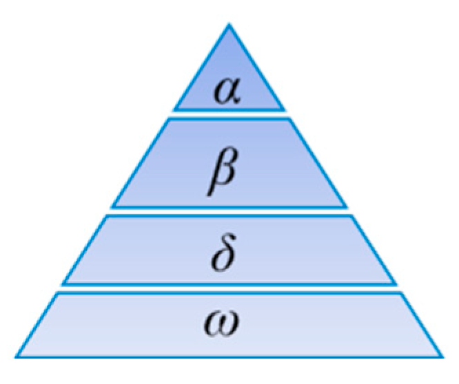
The optimization process of the GWO algorithm is carried out through the collaborative dynamics within a pack of wolves. Within this pack, each wolf assumes a distinct role, establishing a rigid hierarchy, as depicted in Figure 1. The algorithm’s best solution is indicated by the alpha wolf, while the beta wolf and delta wolf denote the secondary and tertiary optimal solutions, respectively. These lead the omega wolf in its search for targets. Throughout the optimization phase, the coordinates of the alpha, beta, delta, and omega wolves are modified [14].

The model of a gray wolf surrounding its prey can be represented by the following equation:

$$D=\left|C\cdot X_n(t)-X(t)\right|$$

(1)

$$X(t+1)=X_p(t)-A\cdot D$$

(2)

In Formula (1), D denotes the geographical distance each wolf maintains from its pursued objective. Formula (2) is the position update formula of wolf pack individuals: in the t-th generation, the symbol $X_p(t)$ denotes the site of quarry, while $X(t+1)$ indicates the site of a wolf during the (t + 1)-th generation. $A$ and $C$ are the coefficients, and the computation procedure is detailed hereafter:

$$A=2a\cdot r_1-a$$

(3)

$$C=2r_2$$

(4)

In this formula, $a$ is the convergence factor, as the iterative process decreases linearly from two to zero. $r_1$ and $r_2$ are random values Between zero and one. $A$ and $C$ are the coefficient vector.

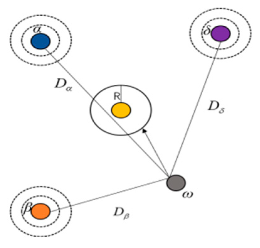
Alpha wolves generally direct the hunt, with the pack’s gray wolves capable of pinpointing and encircling their prey. Within the wolf pack hierarchy, the α wolf, the β wolf and the δ wolf exhibit the keenest awareness of the prey’s probable whereabouts. The positional adjustments of the remaining wolves are guided by the positions of these three dominant individuals. The mathematical model of a gray wolf searching for prey is shown in Figure 2 [15].

$$D_{\alpha }=\left|C_1\cdot X_{\alpha }-X\right|,D_{\beta }=\left|C_2\cdot X_{\beta }-X\right|,D_{\delta }=\left|C_3\cdot X_{\delta }-X\right|$$

(5)

$$X_1=X_{\alpha }-A_1\cdot D_{\alpha },X_2=X_{\beta }-A_2\cdot D_{\beta },X_3=X_{\delta }-A_3\cdot D_{\delta }$$

(6)

$$X(t+1)={\displaystyle \frac{X_1+X_2+X_3}{3}}$$

(7)

In Formula (5), $D_{\alpha }$, $D_{\beta }$, and $D_{\delta }$ denote the distance that separates the ω wolf from the α wolf , the β wolf and the δ wolf, respectively. Formula (6) specifies the orientation and separation between the ω wolf and α wolf, β wolf, δ wolf. Formula (7) denotes a new generation of individual gray wolves.

3. Algorithm Improvement of GWO Algorithm

3.1. Nonlinear Convergence Factor

In the GWO algorithm, nonlinear convergence factors control the hunting process, specifically the search and encircle of prey. When the magnitude of |A| exceeds 1, the gray wolf and prey exhibit a tendency to move apart, suggesting the algorithm’s strength in global optimization. Conversely, when |A| is less than 1, it implies the gray wolf is near the prey, signaling an impending attack, which reflects the algorithm’s proficiency in local exploration. Clearly, a value of |A| greater than 1 indicates a shortcoming in local exploitation, while a value less than 1 signifies a limitation in global search capability [16]. The linear variation cannot be fully adapted to the GWO search process. Therefore, in order to make the convergence factor decrease slowly during the preliminary period and greatly during the subsequent period, this paper makes nonlinear adjustments and uses the Sigmoid function to express

$$a=a_1+{\displaystyle \frac{a_1+a_2}{1+e^{-(2S_{\max }\frac{K-k}{K}-S_{\max })}}}$$

(8)

In Formula (8), $a_1$ and $a_2$ correspond to the lower and upper thresholds of the values. $K$ represents the maximum iteration threshold, and $k$ signifies the iteration count at present. The comparison of convergence factors is demonstrated in Figure 3.

3.2. Adaptive Cross Mutation Strategy

With the intention of bolstering the GWO algorithm’s global exploration capabilities and enriching the diversity within the gray wolf population, an adaptive probabilistic cross mutation strategy has been integrated. In order to prevent premature convergence during the initial iterations, it is essential to elevate the probabilities of crossover and mutation. Conversely, as iterations progress, these probabilities should be decreased to prevent the loss of optimal solutions [17]. Following the adaptive crossover and mutation operations on the initial population, a refreshed population denoted by X’ is generated and merged with the existing gray wolf population X. The fitness of the merged gray wolf individuals is ranked, and the subset with superior fitness—constituting half of the total population—is advanced to the subsequent iteration. The schema for crossover mutation is delineated henceforth:

$$X_1=[x_1^1,x_1^2,\cdot \cdot \cdot ,x_1^{\dim }]$$

(9)

$$X_2=[x_2^1,x_2^2,\cdot \cdot \cdot ,x_2^{\dim }]$$

(10)

$$X_3=[x_3^1,x_3^2,x_3^3,\cdot \cdot \cdot ,x_3^{\dim }]$$

(11)

$$X_1^{\prime }=[x_1^1,x_1^2,x_2^n,\cdot \cdot \cdot ,x_1^{\dim }]$$

(12)

$$X_2^{\prime }=[x_2^1,x_2^2,x_1^n,\cdot \cdot \cdot ,x_2^{\dim }]$$

(13)

$$X_3^{\prime }=[x_3^1,x_3^2,y^n,x_3^{n+1},\cdot \cdot \cdot ,x_3^{\dim }]$$

(14)

In this formula, $X_1$ and $X_2$ denote two gray wolf individuals ready for hybridization. $X_1^{\prime }$ and $X_2^{\prime }$ denote the gray wolf individuals after hybridization. $X_3$ is the gray wolf entity before the mutation occurred. $X_3^{\prime }$ is the gray wolf entity after the mutation occurred. Dim denotes dimension.

The cosine-based adaptive crossover mutation probability formula is outlined below:

$$P_c=\left\{\begin{array}{ll}(P_{c1}+P_{c2})/2\times \cos ((f^{\prime }-f_{avg})/(f_{\max }-f_{avg})\ast \pi /2)& f^{\prime }\ge f_{avg}\\ P_{c1}& f^{\prime }<f_{avg}\end{array}\right.$$

(15)

$$P_m=\left\{\begin{array}{ll}(P_{m1}+P_{m2})/2\times \cos ((f^{\prime }-f_{avg})/(f_{\max }-f_{avg})\ast \pi /2)& f^{\prime }\ge f_{avg}\\ P_{m1}& f^{\prime }<f_{avg}\end{array}\right.$$

(16)

In this formula, $P_{c1}$ and $P_{m1}$ indicate the upper bounds of the crossover and mutation probabilities., respectively. $P_{c2}$ and $P_{m2}$ are the minimum. The individual fitness value is $f^{\prime }$. $f_{avg}$ and $f_{\max }$ represent the mean fitness value and the peak fitness value, respectively.

3.3. Simulated Annealing Operation

During the intermediate and final phases of the GWO optimization, the population of gray wolves often gravitates towards the α wolf, β wolf, and δ wolf. When the α wolf, β wolf, and δ wolf are trapped in a local region while hunting, the entire gray wolf population will fall into a limited search space, hindering further evolutionary progress. Motivated by the strategy of the elite, the algorithm incorporates simulated annealing operations in its later stages to improve the disadvantage of the GWO algorithm easily falling into local optimal in the late stages of optimization [18]. Towards the end of the optimization process, once the fitness of the new wolf pack generation is determined, individuals with the top fitness scores have a certain likelihood of being promoted to the rank of alpha wolf, which effectively decreases the risk of the algorithm getting stuck in local optima during the later period of the algorithm optimization. The principal steps are presented below:

First, the initial temperature and the cooling function are determined:

$$T_0={\displaystyle \frac{f_g(l)}{\log (5)}}$$

(17)

$$T_{l+1}=\lambda T_l$$

(18)

In this formula, $f_g(l)$ stands for the fitness of the best-performing individual (α wolf) in the population for the present iteration. $l$ is the number of cooling. $\lambda$ is the cooling constant.

Then, the probability of accepting the candidate wolf is calculated according to the temperature:

$$P=\exp [-{\displaystyle \frac{f_p(l)-f_g(l)}{T_l}}]$$

(19)

Within this formula, $f_p(l)$ signifies the value of the optimal individual fitness of the wolf pack after l time of cooling.

Finally, the α wolf is updated according to the Metropolis criterion, denoted as

$$g_{best}(l)=\left\{\begin{array}{ll}{p}_{best}(l)& f_p(l)<f_g(l)\\ g_{best}(l-1)& f_p(l)\ge f_g(l)\&P<r\\ p_{best}(l)& f_p(l)\ge f_g(l)\&P\ge r\end{array}\right.$$

(20)

In this formula, r represents a uniformly distributed stochastic variable across the range zero to one. If the optimal individual fitness value $f_p(l)$ after l time of cooling is less than the optimal individual fitness (α wolf) $f_g(l)$, the individual corresponding to $f_p(l)$ is called the α wolf. If the fitness of the optimal individual $f_p(l)$ after l time of cooling is greater than the fitness of the optimal individual (α wolf) $f_g(l)$, then we continue to determine whether the acceptance probability P is greater than the random number r. If $P\ge r$, the individual corresponding to $f_p(l)$ is promoted to α wolf; otherwise, the α wolf from the previous iteration is retained.

3.4. Algorithm Testing and Analysis

The improved algorithm underwent evaluation utilizing seven standard test functions that are widely recognized globally, as shown in

Table 1. International standard test function.

Function	Expression	Search Area	Minimum
Sphere	$f_1\left(x\right)={\displaystyle \sum _{i=1}^D{x}_i^2}$	[−100,100]	0
Schwefel	$f_2\left(x\right)={\displaystyle \sum _{i=1}^D\left|x_i\right|}+{\displaystyle \prod _{i=1}^D\left|x_i\right|}$	[−10,10]	0
Schwefel 1.2	$f_3\left(x\right)={{\displaystyle \sum _{i=1}^D\left({\displaystyle \sum _{j=1}^i{x}_j}\right)}}^2$	[−100,100]	0
Schwefel 2.21	$f_4\left(x\right)={\max }_i\left\{\left|x_i\right|,1\le i\le D\right\}$	[−100,100]	0
Rastrigin	$f_5\left(x\right)={\displaystyle \sum _{i=1}^D\left[x_i^2-10\cos \left(2\pi x_i\right)+10\right]}$	[−5.12,5.12]	0
Six-hump camel back	$\begin{array}{ll}{f}_7\left(x\right)& =4x_1^2-2.1x_1^4+{\displaystyle \frac{1}{3}}{x}_1^6+x_1{x}_2\\ & -4x_2^2+4x_2^4\end{array}$	[−5,5]	−1.03
Ackley	$f_6\left(x\right)=-20\exp \left(-0.2\sqrt{{\displaystyle \frac{1}{d}}{\displaystyle \sum _{i=1}^D{x}_i^2}}\right)-\exp \left({\displaystyle \frac{1}{d}}\sqrt{{\displaystyle \sum _{i=1}^D\cos \left(2\pi i\right)}}\right)+e+20$	[−600,600]	0

. After running 50 experiments, the results were compared with GWO, COGWO, FMGWO, and IGWO to verify the superiority of various performance indexes of the algorithm [19,20,21].

Within the scope of this experimental simulation, the pertinent parameter settings for the GSGWO algorithm are displayed in

Table 2. GSGWO algorithm-related parameters.

$\mathit{N}$	$\mathbf{dim}$	${\mathit{t}}_{\mathbf{max}}$	${\mathit{a}}_1$	${\mathit{a}}_2$	${\mathit{S}}_{\mathbf{max}}$	${\mathit{P}}_{\mathit{c}1}$	${\mathit{P}}_{\mathit{m}1}$	${\mathit{P}}_{\mathit{c}2}$	${\mathit{P}}_{\mathit{m}2}$	$\mathit{\lambda }$
50	30	500	0	2	20	0.8	0.5	0.08	0.05	0.85

.

Table 3. GSGWO and GWO compare the results of seven benchmark functions.

Function	Property	GWO	IGWO	FMGWO	GWO1	GWO2	GSGWO
$f_1$	average	1.25 × 10−58	0	1.64 × 10−150	0	1.47 × 10−105	0
	standard	1.16 × 10−58	0	1.88 × 10−150	0	1.36 × 10−105	0
$f_2$	average	1.46 × 10−30	2.68 × 10−280	1.32 × 10−120	1.56 × 10−300	2.49 × 10−60	1.46 × 10−315
	standard	1.55 × 10−30	6.32 × 10−280	1.49 × 10−119	1.82 × 10−300	1.77 × 10−60	1.83 × 10−315
$f_3$	average	2.96 × 10−40	0	3.49 × 10−135	0	3.55 × 10−70	0
	standard	2.87 × 10−40	0	3.65 × 10−135	0	2.93 × 10−70	0
$f_4$	average	1.24 × 10−35	2.12 × 10−286	1.55 × 10−121	1.67 × 10−267	2.33 × 10−62	1.41 × 10−298
	standard	1.67 × 10−35	1.97 × 10−286	2.33 × 10−122	2.45 × 10−267	1.73 × 10−62	1.23 × 10−298
$f_5$	average	0	0	0	0	0	0
	standard	0	0	0	0	0	0
$f_6$	average	1.73 × 10−14	1.89 × 10−15	1.95 × 10−13	1.55 × 10−14	1.72 × 10−12	1.55 × 10−15
	standard	1.62 × 10−14	2.32 × 10−15	1.32 × 10−13	2.13 × 10−14	1.43 × 10−12	1.32 × 10−15
$f_7$	average	−1.031	−1.022	−1.033	−1.032	−1.030	−1.021
	standard	0	0.001	0.003	0.001	0.01	0.001

presents the average value and standard deviation derived from 50 simulation trials. Among them, GWO1 represents the GWO algorithm improved by the adaptive cross-mutation strategy and simulated annealing operation, and GWO2 represents the GWO algorithm improved by the nonlinear convergence factor only. It can be seen that the GWO1 algorithm performs better on single-peak functions f1-f4 and multi-peak functions f4 and f6, while the traditional GWO algorithm performs poorly on these functions, which verifies the effectiveness of the cross-mutation strategy and simulated annealing operation.

4. DWA Algorithm

The Dynamic Window Approach (DWA) is instrumental in the domain of local path planning algorithms, exerting a significant influence, capable of generating secure paths in real time by taking into account the robots’ dynamic capabilities. Its principle involves establishing a two-dimensional velocity space $\left(v,\omega \right)$ composed of linear and angular velocities. Within a short time interval $\Delta t$, it constructs a search space consisting of feasible trajectories corresponding to all velocities under dynamic constraints. An objective function is then used to opt for the most advantageous trajectory, and the mobile robot is driven according to the corresponding velocities $\left(v,\omega \right)$ for path planning [22,23,24].

The motion state of the mobile robot is described by velocity space $\left(v,\omega \right)$. Assuming that the time interval $\Delta t$ is small and the robot progresses in a straight direction with constant velocity within $\Delta t$, the subsequent kinematic model is presented [25]:

$$\left\{\begin{array}{l}{x}_{t+1}=x_t+v_x\Delta t\cos ({\theta }_t)-v_y\Delta t\sin ({\theta }_t)\\ y_{t+1}=y_t+v_x\Delta t\sin ({\theta }_t)+v_y\Delta t\cos ({\theta }_t)\\ {\theta }_{t+1}={\theta }_t+\omega \Delta t\end{array}\right.$$

(21)

In this formula, $x_t$ and $x_{t+1}$ specify the x-axis locations of the mobile robot at $t,t+1$, respectively. $y_t$ and $y_{t+1}$ specify the y-axis locations of the mobile robot at $t,t+1$, respectively. ${\theta }_t$ and ${\theta }_{t+1}$, respectively, indicate the orientation angle of the mobile robot at $t,t+1$. $v$ indicates linear velocity. $\omega$ expresses angular velocity.

Once the kinematic model has been formulated, the subsequent step involves determining the velocity, essentially developing a model to solve for velocity. In the velocity space $\left(v,\omega \right)$, there is an infinite set of velocity possibilities, which must be narrowed down based on the robot’s actual conditions to derive a viable velocity range:

(1) Velocity constraint:

The robot’s velocity is restricted by the limits of its own speed capacity and the applied safety factor, and its velocity constraint space is characterized by $V_m$:

$$V_m=\left\{(v,\omega )|v\in \left[V_{\min },V_{\max }\right],\omega \in \left[{\omega }_{\min },{\omega }_{\max }\right]\right\}$$

(22)

In this formula, $V_{\min },V_{\max }$ and ${\omega }_{\min },{\omega }_{\max }$ correspond to the minimum and maximum values of the robot’s linear and angular velocities, respectively.

(2) Dynamic constraint:

According to the different motor performance of the applied mobile robot, the acceleration and deceleration speed are different, so it is necessary to apply dynamic performance constraints:

$$V_d=\left\{(v,\omega )|v\in \left[v_c-v_b\Delta t,v_c+v_a\Delta t\right],\omega \in \left[{\omega }_c-{\omega }_b\Delta t,{\omega }_c+{\omega }_a\Delta t\right]\right\}$$

(23)

In this formula, $V_d$ denotes the dynamic constraint space. $v_c$ and ${\omega }_c$ denote the mobile robot’s existing linear and angular velocity. $v_a$ and ${\omega }_a$ express maximum acceleration. $v_b$ and ${\omega }_b$ indicates the maximum deceleration speed.

(3) Braking distance constraints:

To guarantee safety, considering the maximum deceleration requirement, the mobile robot must be able to come to a halt prior to colliding with any obstacle, meaning the velocity should be reduced to 0. $V_a$ represents the braking distance constraint space:

$$V_a=\left\{\left(v,\omega \right)|v\le {\left(2Dis(v,\omega )v_b\right)}^{1/2},\omega \le {\left(2Dis(v,\omega ){\omega }_b\right)}^{1/2}\right\}$$

(24)

In this formula, $Dis(v,\omega )$ denotes the nearest distance between the path related to $\left(v,\omega \right)$ and the obstacle.

And, the objective function assesses the trajectory associated with the velocity space generated under constraints. It primarily includes the cost function $Head(v,\omega )$ of the target position, the cost function $Obs(v,\omega )$ associated with proximity to obstacles, and the speed cost function $Vel(v,\omega )$. Consequently, the aggregate cost function $\mathrm{Cos}t(v,\omega )$ is articulated in the subsequent manner:

$$\mathrm{Cos}t(v,\omega )=\alpha Head(v,\omega )+\beta Obs(v,\omega )+\gamma Vel(v,\omega )$$

(25)

In this formula, $Head(v,\omega )$ denotes the angle between the line segment connecting the mobile robot to the target position and the robot’s current heading. $Obs(v,\omega )$ denotes the minimum distance to the obstacle. $Vel(v,\omega )$ denotes the speed cost of the immediate simulation. $\alpha$, $\beta$, and $\gamma$ are the respective weighting factors applied to the cost functions.

5. Algorithm Improvement of DWA Algorithm

5.1. Adaptive Weights

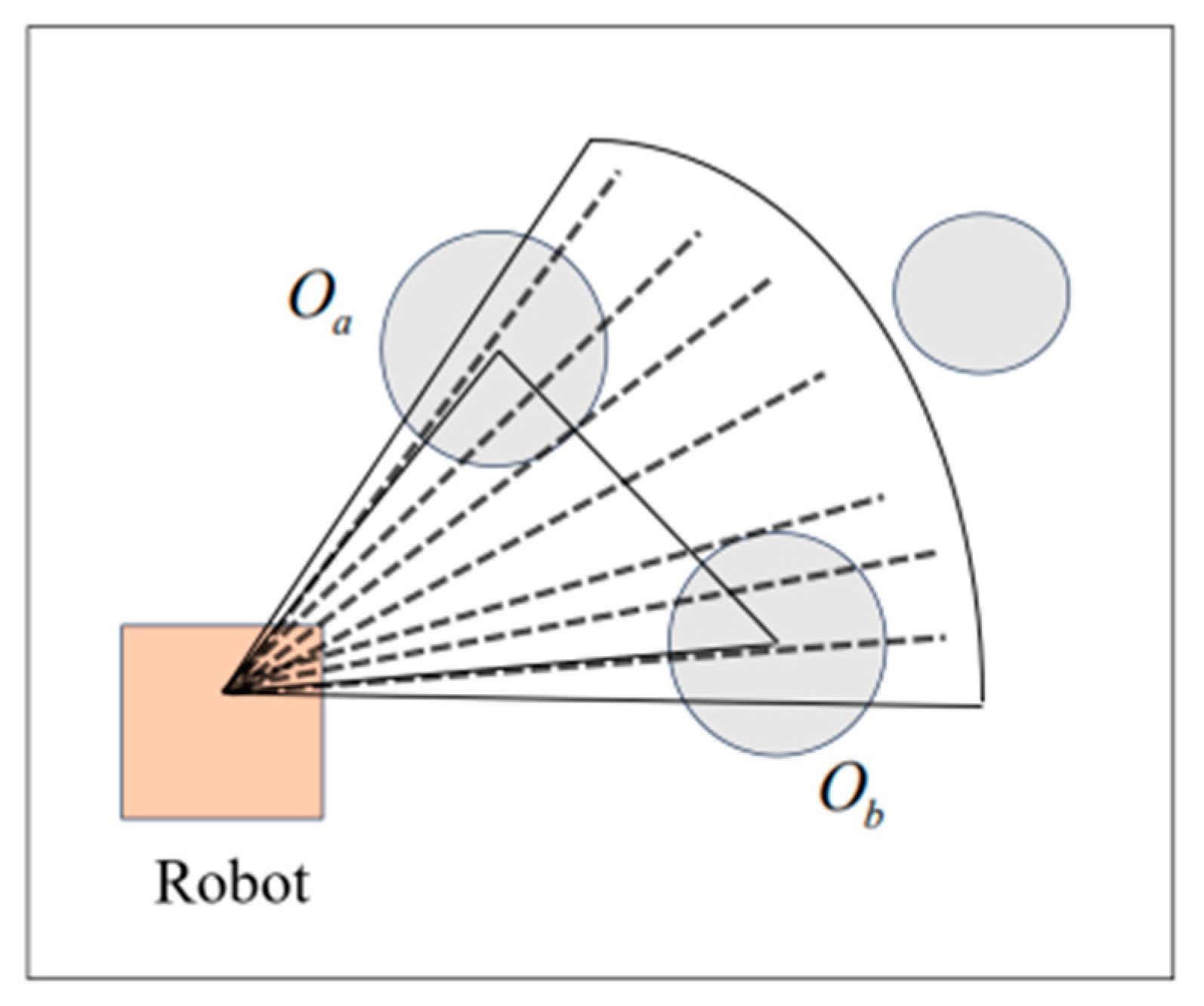
The mobile robot uses lidar to achieve distance measurement functionality. Within lidar’s detection scope, it is capable of determining the distances between the mobile robot and surrounding obstacles. The density of the area is calculated by measuring the distances between obstacles within the detection range. If the gap falls below a predetermined limit, it is classified as a dense obstacle area, and the weights are adjusted in correspondence with the new parameters. The formula for the distance between obstacles is as follows:

$$D_{ab}=\sqrt{Obs{(v,\omega )}_a^2+Obs{(v,\omega )}_b^2-Obs{(v,\omega )}_a\cdot Obs{(v,\omega )}_b\cdot \cos \left({\theta }_a-{\theta }_b\right)}$$

(26)

In Formula (26), $D_{ab}$ denotes the minimal distance between obstacles $O_a$ and $O_b$. $Obs{(v,\omega )}_a$ and $Obs{(v,\omega )}_b$, respectively, indicate the minimal separations among the obstacles. $O_a$ and $O_b$ are the mobile robots. The corresponding heading angles of the mobile robot with respect to obstacles $O_a$ and $O_b$ are denoted as ${\theta }_a$ and ${\theta }_b$, respectively. Figure 4 provides a depiction.

Set the criteria for whether the robot can safely pass by obstacles:

If $D_{ab}>2R_c$, the mobile robot can pass safely. $R_c$ is the expansion radius of the obstacle.

$\mathrm{Obs}{(v,\omega )}_{all}$ represents the set of shortest distances between all obstacles in the sector and the robot. The minimum value $\min \left(Obs{(v,\omega )}_{\mathrm{all}}\right)$ from this set is chosen as the input for the cost function. The ensuing algebraic formulation specifies

$$Obs(v,\omega {)}_{\mathit{all}}=\{Obs(v,\omega {)}_1,Obs(v,\omega {)}_2,\dots ,Obs(v,\omega {)}_n\}$$

(27)

And, the formula for safety distance threshold $D_s$ is

$$D_s=\gamma \cdot \left({\displaystyle \frac{v_{\max }}{v_a}}\right)$$

(28)

In Formula (28), $\gamma$ is the threshold factor. $v_{\max }$ and $v_a$ denote the peak forward speed and linear acceleration capabilities of the mobile robot, respectively. An increase in acceleration correlates with a reduced safety distance threshold, while a higher linear velocity is associated with an increased safety distance threshold.

If $\min \left(Obs{(v,\omega )}_{\mathrm{all}}\right)$ is greater than $D_s$, there is no necessity to decrease the speed, so the parameters of the speed function can be set to the maximum value.

If $\min \left(Obs{(v,\omega )}_{\mathrm{all}}\right)$ is less than or equal to $D_s$, introduce the adaptive parameter $\xi$ to control the speed function, as shown in the following formula:

$$\xi =\left\{\begin{array}{l}{\xi }_{\min }+\left({\xi }_{\max }-{\xi }_{\min }\right)\cdot \sin \left({\displaystyle \frac{\min \left(Obs{(v,\omega )}_{all}\right)}{D_s}}\right),\min \left(Obs{(v,\omega )}_{all}\right)\le D_s\hfill \\ {\xi }_{\max },\min \left(Obs{(v,\omega )}_{all}\right)>D_s\hfill \end{array}\right.$$

(29)

In Formula (29), the range of $\xi$ is $\left[{\xi }_{\min },{\xi }_{\max }\right]$ with ${\xi }_{\min }$ and ${\xi }_{\max }$ corresponding to the values for successfully passing through densely packed obstacles and for passing through areas with a higher density of obstacles in the shortest time, respectively. The weighted coefficient of the speed function in the traditional DWA algorithm’s cost function is replaced by the improved adaptive weights.

5.2. Offset Evaluation Function

Incorporating adaptive weights into the velocity function, a novel offset evaluation function $\mathrm{Mis}(v,\omega )$ is proposed to ensure that the Dynamic Window Approach (DWA) better aligns with the optimal trajectory generated by the improved global path planning algorithm (GSGWO). This function assesses the degree by which the local path generated by the DWA algorithm deviates from the global optimal path. It ensures that while achieving local obstacle avoidance and path planning, the generated trajectory follows the global path with the highest possible precision.

The offset evaluation function $\mathrm{Mis}(v,\omega )$ serves to determine the smallest gap between the anticipated trajectory of the DWA algorithm at a given position and the global path. The cluster of nodes in the path generated by the global path planning algorithm is represented as $P_{\mathrm{global}}=\left\{\left(x_1,y_1\right),\left(x_2,y_2\right),\dots ,\left(x_k,y_k\right)\right\}$, with a total of K nodes. The projected positional coordinates derived from the DWA at time $t$ is $\left(x_t,y_t\right)$. The corresponding equation is articulated subsequently:

$$Di{s}_k^t=\sqrt{{\left(x_t-x_k\right)}^2+{\left(y_t-y_k\right)}^2}$$

(30)

$$Di{s}^t=\left\{{\mathrm{Dis}}_1^t,\right.{\mathrm{Dis}}_2^t,\dots ,Di{s}_k^t\}$$

(31)

$$\mathrm{Mis}(v,\omega )=\min \left(Di{s}^t\right)$$

(32)

In this formula, $x_t$, $y_t$ are the horizontal and vertical coordinates, respectively, of the approximated location of the DWA algorithm at time $t$, while $x_k$, $y_k$ are the horizontal and vertical coordinates, respectively, of the $k$-th node in the path. $Di{s}_k^t$ represents the Euclidean distance between the approximated location of the DWA algorithm at time (t) and the $k$-th node in the path. $Di{s}^t$ is the set of distances to the nodes.

Based on this, the refined cost function $N\mathrm{Cos}t(*)$ is hereby specified:

$$N\mathrm{Cos}t(v,\omega )=\alpha \mathrm{Head}(v,\omega )+\beta \mathrm{Obs}(v,\omega )+\xi \mathrm{Vel}(v,\omega )+\phi Mis(v,\omega )$$

(33)

In Formula (33), $Head(v,\omega )$ denotes the deviation in angle between the line from the robot to the target and the robot’s current directional heading. $Obs(v,\omega )$ denotes the smallest distance to the obstacle. c represents the speed cost of the current simulation. $\alpha$, $\beta$, $\xi$, and $\phi$ are the respective weighting factors applied to the cost functions.

6. Fusion Algorithm Based on GSGWO and IDWA

The improved GWO algorithm enhances the capacity of global path planning, but only for static environments, and there are cusps in the path. The DWA algorithm is a well-established local path planning algorithm with strong practicability, but it is prone to getting stuck in local optima and lacks a global perspective. After optimizing the GWO algorithm, it further adopts the DWA algorithm to execute real-time evasion of obstacles in a dynamic environment, while optimizing the path’s smoothness to satisfy the robot’s motion performance, and puts forward a fusion algorithm building upon the improved Gray Wolf Algorithm (GSGWO) and improved DWA (IDWA) [26,27,28].

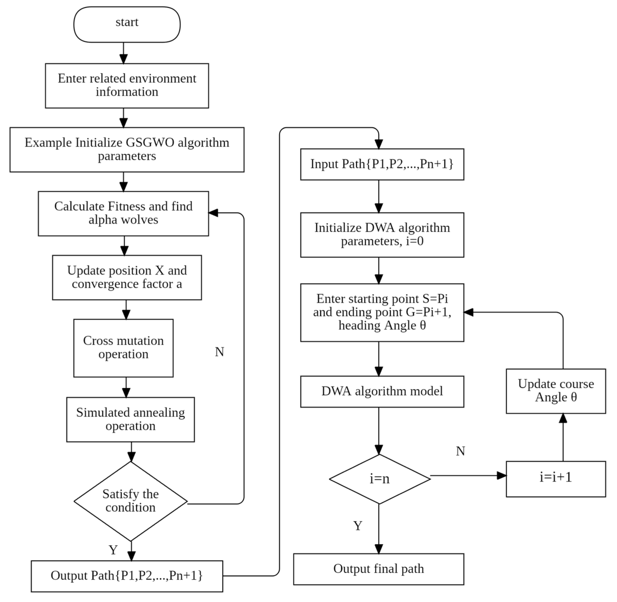
The underlying mechanism behind the fusion algorithm is as follows: The GSGWO algorithm is applied to derive a global trajectory, followed by the extraction of critical nodes as local target locations. The primary factor influencing the trajectory’s smoothness is heading angle. Therefore, the initial heading angle inherits the heading angle that reached the local target point last time when the IDWA algorithm is implemented to design the robot’s local path, to therefore ensure the smoothness of the path. The flow chart is depicted in Figure 5.

The detailed execution procedure is outlined below:

• Initialize the parameters of the GSGWO algorithm for global path planning.
• Utilize the GSGWO algorithm to calculate fitness and identify the alpha wolves, which represent the best solutions in the current iteration.
• Update position X and convergence factor a within the GSGWO algorithm.
• Perform crossover mutation and simulated annealing operations to avoid local optima and enhance solution diversity until the termination condition is met, and then, generate the global path.
• Extract the key node $\left\{P_0,P_1,\dots P_{n+1}\right\}$ of the global path serving as the local target, and the initiation of each local trajectory is $S\left\{S_1,S_2,\dots S_n\right\}=\left\{P_0,P_1,\dots P_n\right\}$. Each local target point is $G\left\{G_1,G_2,\dots G_n\right\}=\left\{P_1,P_2,\dots P_{n+1}\right\}$, and the path is divided into n local paths composed of $\left\{S_1{G}_1,S_2{G}_2,\dots S_n{G}_n\right\}$.
• For the local path $S_1{G}_1$, the IDWA algorithm is utilized to determine the trajectory, and the velocity space $\left(v,\omega \right)$ and course angle ${{\theta }_1}^s$ (referring to the course angle at the starting point $S_1$) are initialized. A 2D velocity space $\left(v,\omega \right)$ comprising linear and angular components is established.
• Build the robot kinematic model.
• The ideal path is chosen based on the criteria defined by the objective function $\mathrm{Cos}t$, and the corresponding speed $(v,\omega )$ is used to drive the mobile robot for path planning. Record the heading angle ${{\theta }_1}^G$ when the robot reaches $G_1$.
• The IDWA algorithm is utilized for the trajectory $S_2{G}_2$, and the initial heading angle of ${{\theta }_2}^S={{\theta }_1}^G$, that is, the second path’s local path planning retains the orientation angle from the prior phase to ensure the smoothness of the generated path.
• The IDWA algorithm is repeatedly utilized for the trajectory $S_3{G}_3,\dots S_n{G}_n$ successively.
• Record the planned route $\left\{S_1{G}_1,S_2{G}_2,\dots S_n{G}_n\right\}$, and finally, output the complete path.

7. Experimental Simulation and Analysis

The experimental setup for this algorithm utilizes a 64-bit WIN10 operating system with a memory capacity of 16G, and the experimental platform is MATLAB 2016. In order to maintain a good comparison effect, the commencement and termination points of the route in the experiment are, respectively, (0,0) and (10,10). The subsequent parameters are detailed in

Table 4. DWA-related parameters.

Maximum Linear Velocity	Minimum Linear Velocity	Maximum Angular Velocity	Maximum Linear Acceleration	Maximum Angular Acceleration	Sampling Period
1.5 m/s	0 m/s	30°/s	0.2 m/s2	40°/s2	0.1 s

:

7.1. Global Path Planning

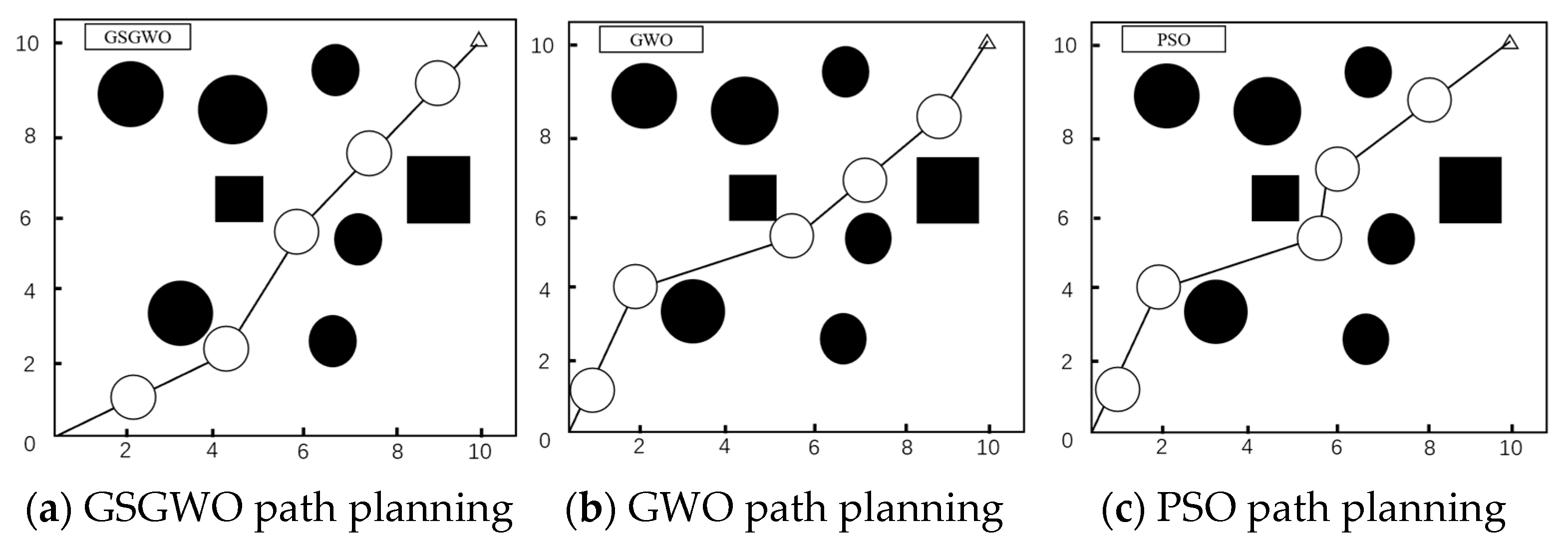
The experimental procedure is initiated within the parameters defined by Scenario 1, which entailed a comparison of the algorithm’s path planning performance against both the conventional GWO and PSO algorithms. Scenario 1 was a mixed map of black solid squares and black solid round obstacles, with a total of eight obstacles. And, the black hollow circles represent robots of a certain size. Owing to the high density of these obstacles, the algorithm was configured to use five path nodes. The classical test function is used to train the algorithm, and it was established that the enhanced version of the GSGWO algorithm is capable of attaining the optimal solution under a small population. Consequently, the aggregate number of individuals in the population becomes 20 and the supreme number of iterations becomes 100.

Figure 6 illustrates the optimal paths of several algorithms. Among them, the black solid squares and black solid round obstacles represent obstacles. The combination of black hollow circles and curves represents the path planned by robots and the triangle represents the endpoint. One can observe that the GWO algorithm and PSO algorithm have larger turning angles and fall into local optima, while the GSGWO algorithm generates smoother paths.

Table 5. Simulation result.

Algorithm	Average Fitness	Optimum Fitness	Worst Fitness	Standard Deviation
GSGWO	14.95	14.50	15.51	0.62
GWO	17.32	14.91	19.20	2.35
PSO	16.87	15.53	20.01	1.52

lists the average fitness, optimum fitness, worst fitness, and standard deviation of the outcomes of fifty runs. It is observable that relative to conventional heuristic methods, the GSGWO algorithm has a better path optimization ability, a shorter generated path length, a smaller standard deviation, and better stability.

7.2. Local Path Planning

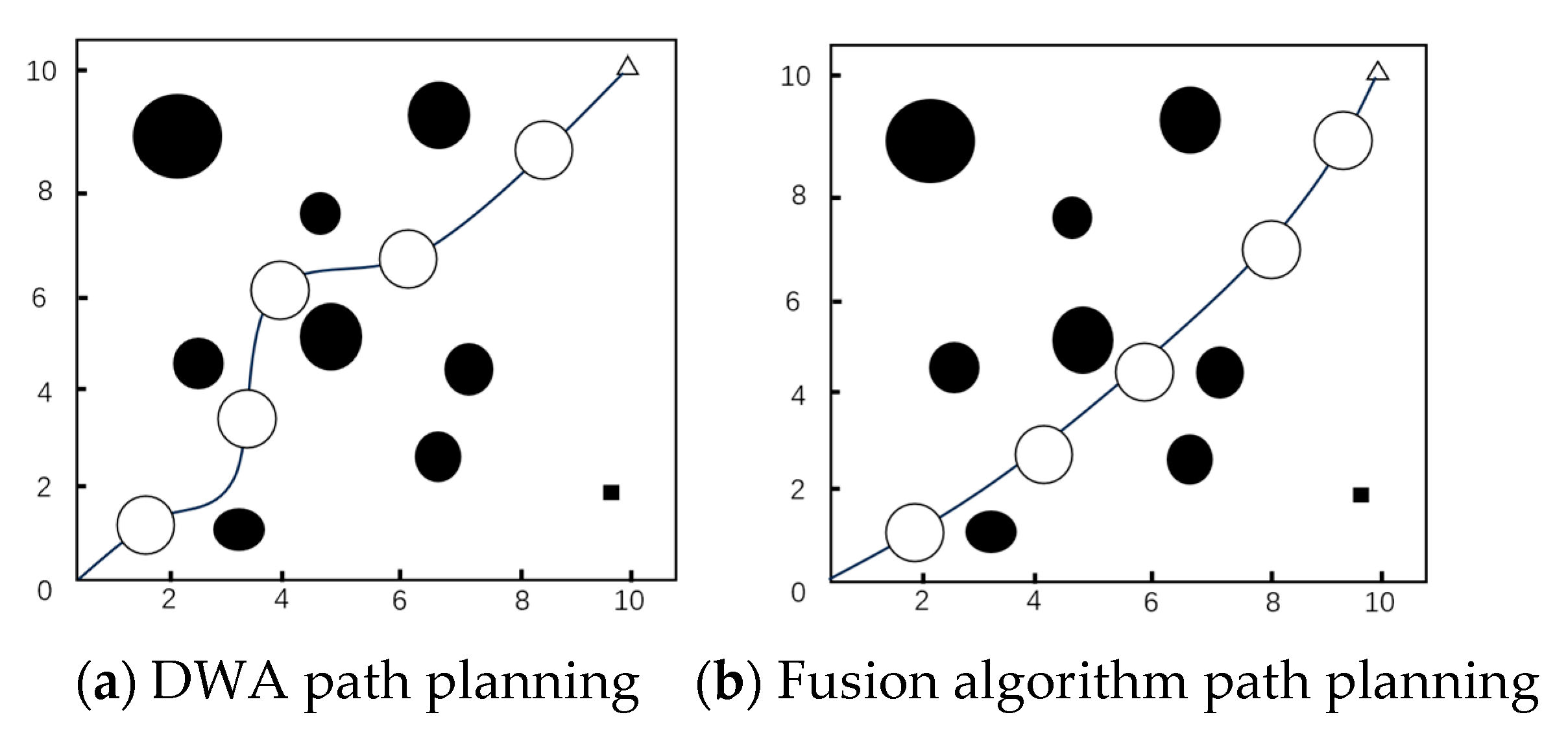
In this experiment, the algorithm of fusion of the improved GSGWO and IDWA algorithm is substantiated by experimental results and subjected to a comparative analysis with the traditional dynamic window method in Scenario 2. Scenario 2 is a hybrid map of both fixed and moving obstacles, with eight static black solid round obstacles and a black solid square obstacle moving uniformly to the left. And, the black hollow circles represent robots of a certain size. The commencement and termination points of the route in the experiment are (0,0) and (10,10), respectively.

In Figure 7, the black solid squares and black solid round obstacles represent obstacles. The combination of black hollow circles and curves represents the path planned by robots and the triangle represents the endpoint. As illustrated in Figure 7a, the path obtained by the DWA algorithm gets stuck in local optimal, which, despite being smooth, contains redundant sections. Figure 7b shows that subjected to a comparative analysis with the traditional algorithm, the path generated by the fusion algorithm is significantly shorter and has higher path smoothness. The fusion algorithm improves the problem of poor smoothness and real-time performance of the global path planning algorithm and overcomes the issue of local path planning algorithms being prone to getting stuck in local optima, and the generated path conforms to the robot kinematic model.

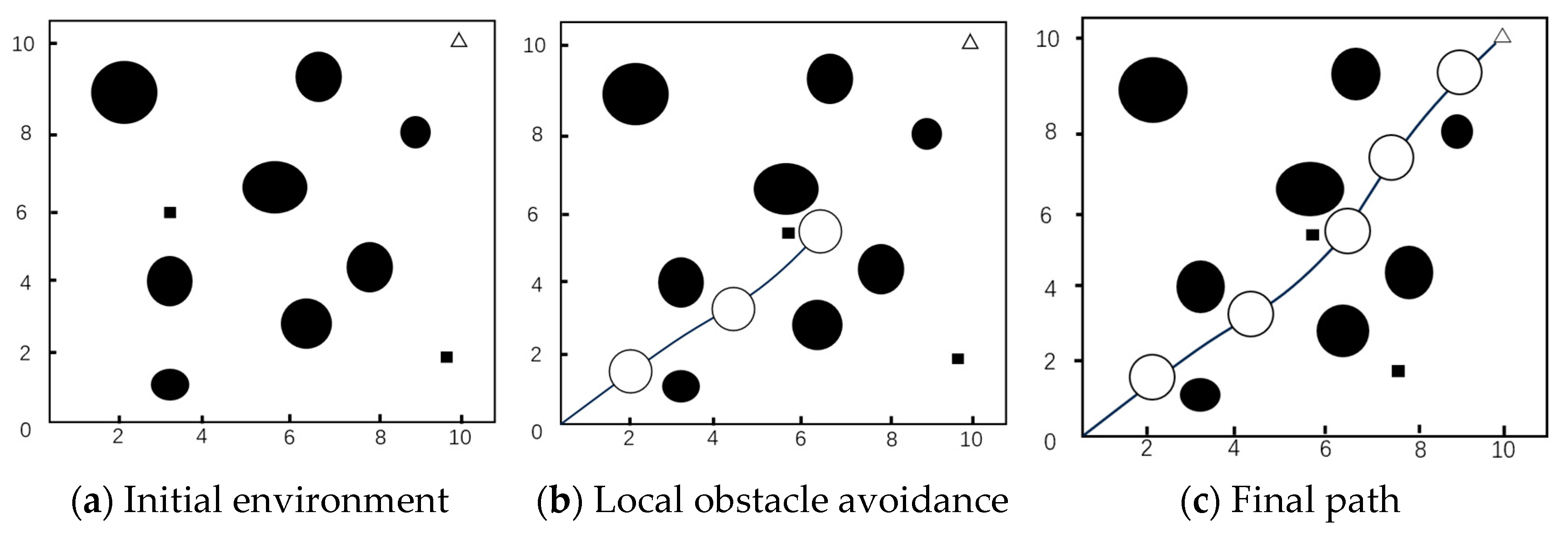
With the intention to evaluate the performance of the fusion algorithm more comprehensively, the number of dynamic obstacles is increased for experimental testing. By modeling a higher degree of environmental complexity, we observe how the algorithm performs against multiple dynamic obstacles. During the experiment, the path planning results of the fusion algorithm under multiple moving obstacles were recorded, and the corresponding path diagram was depicted, as illustrated in Figure 8. Among them, the black solid squares and black solid round obstacles represent obstacles. The combination of black hollow circles and curves represents the path planned by robots and the triangle represents the endpoint.

As is observable in Figure 8b, when encountering dynamic obstacles, the path can quickly be adjusted and avoid the obstacles immediately. Figure 8c shows the final path graph generated by the fusion algorithm.

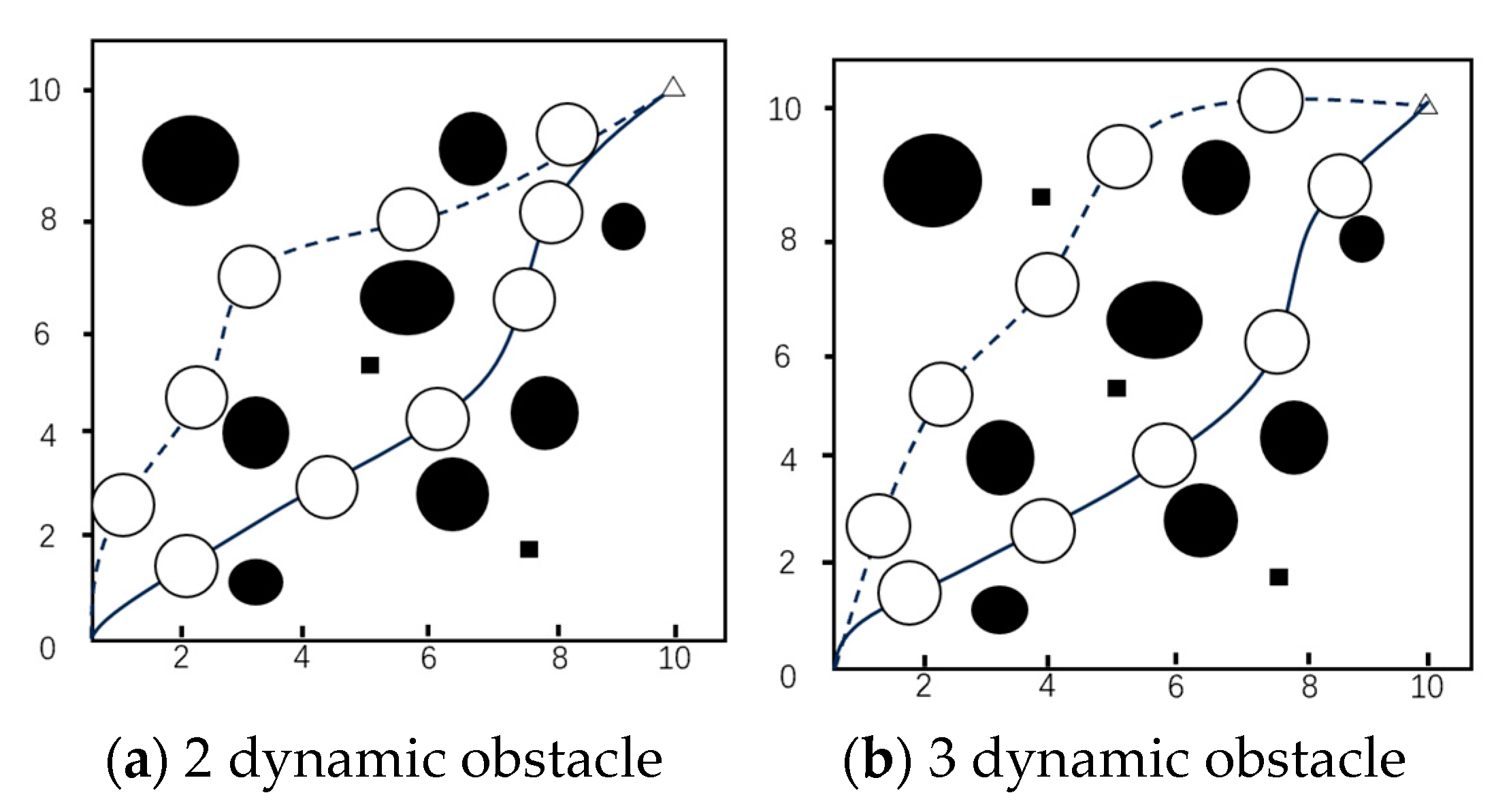
After continuing to increase the number of dynamic obstacles and observing the path planning capabilities of the DWA and fusion algorithm, the delineated trajectory’s extent is depicted within Figure 9. Among them, the black solid squares and black solid round obstacles represent obstacles. The combination of black hollow circles and curves represents the path planned by robots and the triangle represents the endpoint. The dashed curve is used to mark the path generated by the traditional DWA algorithm, while the solid curve is used to represent the path generated by the new algorithm after fusion.

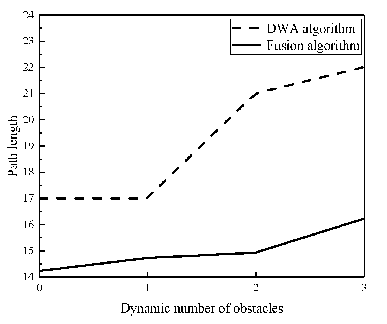
Figure 10 shows the path length variation diagram.

Figure 10 demonstrates that with the increase in obstacles, the path generated by the traditional DWA algorithm increases significantly, while the fusion algorithm has little change in path length, high stability, and strong ability to pass through dense obstacle areas when obstacles increase. The experimental outcomes thoroughly confirm the efficacy of the improved algorithm.

7.3. Experimental Scenario Verification

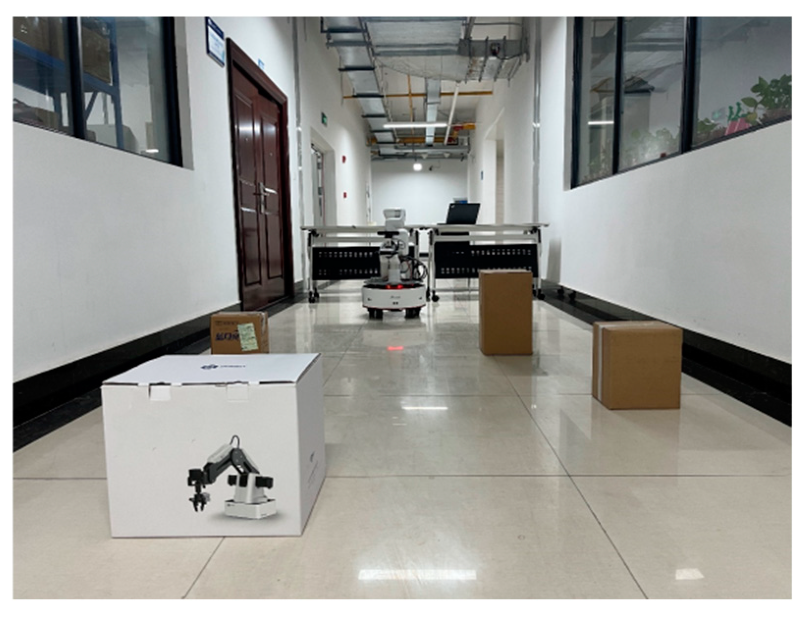
An indoor environment with obstacles arranged in the corridor as depicted in Figure 11 was constructed. On the Ubuntu 16.04 platform, path planning was implemented for an autonomous robot utilizing the Robot Operating System (ROS). Initially, it was connected to the Wi-Fi signal emitted by the mobile robot to communicate with the host. Then, lidar was used to build a map of the experimental scenario, and map visualization was implemented. After that, global localization was conducted for the mobile robot. Figure 12 shows a map constructed using a laser radar (Shenzhen Yuedeng Intelligent Technology Co., Ltd., Shenzhen, China), where the regions of black areas indicate the locales of impediments.

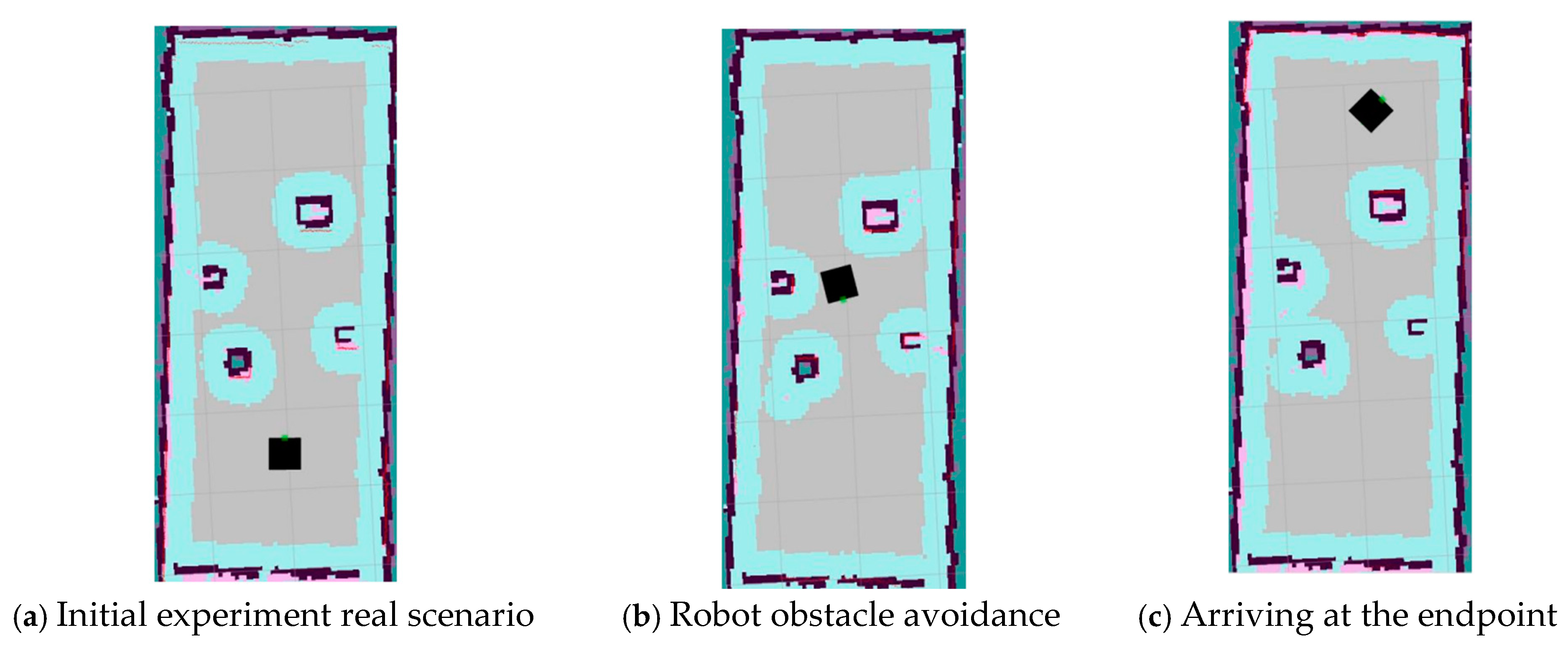
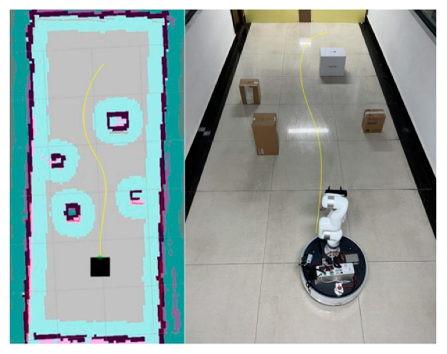
The path planning results in the real scenario are shown in Figure 13, with the black square indicating the mobile robot’s placement and the dark red regions denoting the obstacles’ presence. The yellow curve represents the optimal path planned by the mobile robot using the path planning algorithm.

As represented in Figure 14, the mobile robot successfully made its way to the target position along the planned trajectory, and empirical trials have conclusively substantiated the efficacy of the refined algorithm.

8. Conclusions

Firstly, a novel iteration of the GSGWO algorithm is introduced to address the inherent limitations of traditional global path planning methodologies, including slow convergence velocities, diminished precision, and constraints to static environmental conditions. Initially, an adjustable nonlinear convergence factor is used to search and optimize the balance of the algorithm during its initial phase. At the same time, an adaptive genetic hybridization strategy is adopted to breed new individuals in pairs with a certain probability, so as to broaden the diversity of the gray wolf population in an effective manner. The simulated annealing operation is used to accept the candidate wolves in the later iterations, preventing the algorithm from becoming trapped in local optima. The GSGWO algorithm is tested on the classical test function, and the data demonstrate that the proposed algorithm has higher optimization ability and stability than other optimization algorithms. Ultimately, the GSGWO algorithm is subjected to a comparative analysis with other path planning algorithms, with experimental results demonstrating its superiority in terms of faster iterative speeds and enhanced optimization capabilities.

Then, aiming at the problems of local path planning algorithm, such as poor possibility and unreachable targets in dense environments and building upon the foundational principles of the conventional DWA algorithm, this study presents an improved IDWA algorithm. The algorithm divides the map into a dense obstacle map and a sparse obstacle map and adds adaptive weights for speed constraints. The offset evaluation function is added to the objective function for cost to make the generated path as close as possible to the global path planning trajectory.

Finally, the GSGWO algorithm and IDWA algorithm are integrated to ensure that the mobile robot has a global planning ability and local obstacle avoidance. The proposed algorithm is applied to the built simulation experiment environment for test verification and compared with the traditional DWA algorithm. Dynamic obstacle avoidance tests are carried out by continuously adding dynamic obstacles. The test data reveal that the algorithm exhibits better abilities of path optimization and obstacle avoidance.