Variable-Step-Size Generalized Maximum Correntropy Affine Projection Algorithm with Sparse Regularization Term

Abstract

Adaptive filtering plays a pivotal role in modern electronic information and communication systems, particularly in dynamic and complex environments. While traditional adaptive algorithms work well in many scenarios, they do not fully exploit the sparsity of the system, which restricts their performance in the presence of varying noise conditions. To overcome these limitations, this paper proposes a variable-step-size generalized maximum correntropy affine projection algorithm (C-APGMC) with a sparse regularization term. The algorithm leverages the system’s sparsity by using a correlated entropy-inducing metric (CIM), which approximates the l₀ norm of the norms, assigning stronger zero-attraction to smaller coefficients at each iteration. Moreover, the algorithm employs a variable-step-size approach guided by the mean square deviation (MSD) criterion. This design seeks to optimize both convergence speed and steady-state performance, improving its adaptability in dynamic environments. The simulation results demonstrate that the algorithm outperforms others in echo cancellation tasks, even in the presence of various noise disturbances.

1. Introduction

In the field of speech signal processing, adaptive filters can adjust the parameters in real time according to the changes in the input signal to better adapt to the non-stationary signals and unknown system environment [1,2,3], so they have been more widely used in the fields of acoustic echo cancellation and active noise control [4,5,6]. Adaptive filtering methods, including the least mean square (LMS) algorithm based on the minimum mean square error (MSE) criterion and the normalized least mean square (NLMS) algorithm, are widely used due to their relatively short data training time requirements [7,8,9]. The affine projection (AP) algorithm, which uses recycled input signals to speed up convergence, was a significant advancement. Since then, AP-based algorithms have become the dominant choice in adaptive filtering [10].

In order to optimize the robustness of AP class algorithms, researchers have proposed constrained optimization criterion algorithms such as the symbolic algorithm (SA) and maximum entropy criterion (MCC) algorithm [11,12,13], combined them with AP algorithms in terms of the cost function, and proposed the APSA algorithm and APMCC algorithm with strong robustness [14,15]. Recently, the generalized maximum correlation entropy affine projection (APGMC) algorithm was introduced. It is based on the generalized correlation loss (GC-loss) function, which helps to lower the algorithm’s complexity [16,17]. Similarly, the recently discovered variable projection order (VPO) method is able to reduce the computational complexity associated with a fixed projection order and is widely used in AP algorithms [18,19,20,21].

However, the use of sound-absorbing materials in indoor environments, as well as directional microphone technology that captures sound only in a specific direction, has weakened the effects of multipath propagation of signals, resulting in a decreasing number of echo paths, which leads to an increasingly sparse echo channel. The upgrading of hardware technology has posed a comparative challenge to the development of system algorithms, and the traditional algorithms mentioned above may suffer from performance issues in certain applications. This is due to the challenge of precisely identifying a small set of critical parameters within the system [22]. In this regard, some researchers found that the zero-attraction factor l₀-paradigm or l₁-paradigm constructed from the low-order paradigm of the weight vector can reduce the error of the algorithms in sparse systems [23] and proposed the zero-attraction LMS (ZA-LMS) algorithm, the reweighted zero-attraction LMS (RZA-LMS) algorithm, the l₀-paradigm LMS (l₀-LMS) algorithm, polynomial ZA-LMS (PZA-LMS) algorithm, and so on [24,25,26,27].

However, there are not many applications of zero-attraction factor in AP algorithms, and the existing algorithms struggle to balance the steady-state error, convergence speed, and computational complexity [28]. For example, the zero-attraction affine projection notation (APSAZA) algorithm has a simple structure but struggles to obtain a low steady-state error [29]. The maximum correlation entropy affine projection with correlation entropy-induced metric (APMCCCIM) algorithm [30] and the correntropy-based affine projection algorithm with compound inverse proportional function (APMCCCIPF) are more computationally complex due to the inclusion of the matrix inversion process [31].

This paper proposes a variable-step generalized maximum correlation entropy affine projection algorithm (C-APGMC) with a sparse penalty term. In the short name of the algorithm, the first ‘C’ denotes the sparse regularization term added by the algorithm, i.e., the associated entropy-inducing metric. The algorithm uses the correlation entropy-induced metric (CIM), which approximates the l₀-paradigm, as the paradigm penalty term. The overall algorithm can better exploit the sparse nature of echo paths while keeping the complexity low. The above advantages of the algorithm indicate that it is suitable for sparse channel identification for indoor online meetings and can solve the sparse channel echo cancellation problem in this scenario due to the environmental arrangement and hardware technology upgrades. In addition, the mean square deviation (MSD) of the algorithm can measure the average error between the output signal and the desired signal, thus establishing a link between the algorithmic step size and the current error and coordinating the algorithm’s performances. Thus, this approach will be applied in this paper to derive a formula for the variable step size in the proposed algorithm. This method solves the problem that current algorithms struggle to weigh the computational complexity and specific performance. As verified by simulation experiments, the proposed algorithm in this paper outperforms many existing algorithms in most aspects.

This paper consists of the following sections: Section 2 discusses the application model of the algorithms as well as the existing base algorithms. Section 3 discusses the algorithms proposed in this paper and their implementation process. Section 4 provides a steady-state analysis of the algorithm. Section 5 provides a complexity analysis of the algorithm. In Section 6, several related algorithms are compared and simulated in terms of sparse system identification and echo cancellation. Section 7 is the conclusion.

2. Overview of Existing Related Algorithms

2.1. Algorithmic Model

The adaptive algorithm employs a feedback mechanism to continuously adjust the weight vector in response to the error signal e(n), generated in each iteration [3]. This enables the output signal to remain in close proximity to the desired signal d(n), which is derived from Equation (1).

$$d\left(n\right)=x^T\left(n\right)w_0+v\left(n\right)$$

(1)

where the input signal is x(n) = [x(n), x(n − 1), …, x(n − k + 1)]^T, w₀ = [w₁, w₂, …, w_k]^T denotes the weight vector of the system to be recognized, v(n) denotes the background noise, the parameter k is a real number that denotes the total length of the system to be detected, and T represents the transposition of the vector or matrix. Based on the output signal y(n) at moment n, the system error e(n) for this iteration is obtained as

$$e\left(n\right)=d\left(n\right)-y\left(n\right)=d\left(n\right)-x^{\mathrm{T}}\left(n\right)w\left(n\right)$$

(2)

In Equation (2) w(n) represents the weight vector. In the application of adaptive algorithms in system identification, the ultimate goal is to iteratively update w(n) so that it constantly approximates the weight vector w₀ of the system to be detected.

2.2. AP Algorithm

The affine projection (AP) algorithm accelerates convergence by reusing input signals in the adaptive process, in which the input signal matrix is X(n) = [x(n), x(n − 1), …, x(n − P + 1)], the matrix size is k × P, where P is the projection order of the AP algorithm and k denotes the filter length. The algorithm can be expressed by the following constrained optimization law:

$$\underset{w\left(n+1\right)}{\min }{‖w\left(n+1\right)-w\left(n\right)‖}_2^2\mathrm{s}.\mathrm{t}.d\left(n\right)-X^T\left(n\right)w\left(n+1\right)=0$$

(3)

where ||·||₂ denotes the l₂-paradigm and the expected signal d(n) = [d(n), d(n − 1), …, d(n − P + 1)]^T, from which the recursive formula of the AP algorithm is given as

$$w\left(n+1\right)=w\left(n\right)+\mu X\left(n\right){\left[X^{\mathrm{T}}\left(n\right)X\left(n\right)\right]}^{-1}e\left(n\right)$$

(4)

where e(n) = [e(n), e(n − 1), …, e(n − P + 1)]^T is the error signal, μ denotes the algorithm step size (i.e., learning rate). The algorithm has a faster convergence speed in a Gaussian environment, but it is less robust because it does not have higher-order statistics and is not suitable for sparse-system-related applications.

2.3. APGMC Algorithm

To enhance the adaptability of the AP algorithm in non-Gaussian noise environments, the APGMC algorithm was proposed. This method integrates the AP algorithm with the GC-loss function, utilizing the generalized maximum correlation entropy (GMC) criterion and imposing a constraint on the filtering vectors, namely,

$${\min }_{w\left(n\right)}{\displaystyle {\sum }_{j=0}^{P-1}\stackrel{\wedge }{J_{GC}^1}\left(e_p\left(n-j\right)\right)=\gamma P-{\displaystyle {\sum }_{j=0}^{P-1}\exp \left(-\lambda {\left|e_p\left(n-j\right)\right|}^{\alpha }\right)}}\mathrm{s}.\mathrm{t}.{‖w\left(n\right)-w\left(n-1\right)‖}_2^2\le {\mu }^2$$

(5)

where e_p(n − j) = y(n − j) − x^T(n − j) w(n) denotes the posteriori error, γ, λ, and α are scalars controlling the size as well as the shape of the kernel function, and μ² is a parameter used to ensure that the weights’ error vector has less energy between two consecutive instantaneous times. According to [17], the weights of this algorithm can be obtained as

$$w\left(n\right)=w\left(n-1\right)+\mu {\displaystyle \frac{X\left(n\right)B\left(n\right)\mathrm{sgn}\left(e\left(n\right)\right)}{{‖X\left(n\right)B\left(n\right)\mathrm{sgn}\left(e\left(n\right)\right)‖}_2}}$$

(6)

The matrix B(n) = diag[b(n), b(n − 1), …, b(n − P + 1)] is a diagonal with elements b(n − j), j∈ {1, 2, …, P − 1} of a diagonal matrix, where b(n − j) = exp(−λ|e_p(n − j) |^α) |e_p(n − j) |^α−1. Note that the a posteriori error e_p(n − j) in both B(n) and sgn(e_p(n)) above is unknown and related to w(n), so it cannot be estimated directly until w(n) is known and thus can be replaced by e(n − j) = d(n − j) − x^T(n − j) w(n − 1) as an approximation. The system identification simulation results in the literature [17] show that APGMC has stronger robustness and effectiveness than other existing AP-like algorithms. However, it is difficult to apply in sparse systems such as acoustic echo paths due to its lack of a sparse penalty term.

3. C-APGMC Algorithm and Its Implementation

3.1. Cost Function Analysis

In order for the APGMC algorithm to be applied to sparse systems, the algorithm can be made to incorporate the l₀-paradigm that is best suited to measure the sparsity of the system. So, the correlation entropy-induced metric (CIM) is employed as an approximate l₀-paradigm to provide a measure of sparsity. This is achieved by quantifying the correlation and uncertainty of the signal. The metric can be expressed as

$$\mathrm{CIM}\left(X,Y\right)=E{\left(\kappa \left(0\right)-\stackrel{\wedge }{V}\left(X,Y\right)\right)}^{1/2}$$

(7)

The entropy of correlation of random variables X and Y, which comprise k samples, can be approximated as

$$\stackrel{\wedge }{V}\left(X,Y\right)={\displaystyle \frac{1}{k}}{\displaystyle \sum _{i=1}^k\kappa \left(x_i,y_i\right)}$$

(8)

In the framework of correlation entropy, the choice of the kernel function affects the way the data are distributed in the mapping space and thus the final calculated metric. Different kernel functions take different approaches to data mapping, which can affect the balance between local and global relationships. Gaussian kernel functions increase the non-linear relationship between the data in a high-dimensional way, enhancing the ability to capture the local structure of the data. In the field of sparse system identification, the Gaussian kernel function is more sensitive to a small number of important coefficients than other kernel functions and can correctly reflect a small amount of system parameter information of the echo channel, which is widely used in the field of echo cancellation. Typically, the Gaussian kernel function in the correlation entropy induction metric can be expressed as

$$\kappa \left(x,y\right)={\displaystyle \frac{1}{\sigma \sqrt{2\pi }}}\exp \left(-{\displaystyle \frac{e^2}{2{\sigma }^2}}\right)$$

(9)

In Equation (7), $\kappa \left(0\right)=1/\sigma \sqrt{2\pi }$, σ is the kernel width of the CIM and e = x − y. For any random variable X = [x₁, x₂, …, x_k]^T, the constructed approximate l₀-paradigm expression is as follows

$${‖X‖}_0\sim {\mathrm{CIM}}^2\left(X,0\right)={\displaystyle \frac{\kappa \left(0\right)}{k}}{\displaystyle \sum _{i=1}^k\left(1-\exp \left(-\frac{x_i^2}{2{\sigma }^2}\right)\right)}$$

(10)

From Equation (10), if |x_i| > δ (δ is a positive constant close to zero) and ∀x_i ≠ 0, the result can be arbitrarily close to the l₀-paradigm as σ → 0. Since it is related to the correlation entropy, this non-linearity measure is called the correlation entropy-induced measure. The corresponding cost function in this paper is

$$J_{CIM}={\displaystyle \frac{1}{k\sigma \sqrt{2\pi }}}{\displaystyle \sum _{j=1}^k\left(1-\exp \left(-\frac{w_j^2\left(n\right)}{2{\sigma }^2}\right)\right)}$$

(11)

The methodological soundness of using the correlation entropy induction metric as a cost function for sparse penalty terms has been demonstrated in the literature [32]. The cost function for the proposed algorithm is then derived as follows:

$$\begin{array}{c}J\left(w\left(n\right)\right)=J_{\mathrm{APGMC}}\left(w\left(n\right)\right)-\beta J_{\mathrm{CIM}}=\gamma P-{\displaystyle \sum _{j=0}^{P-1}\exp \left(-\lambda {\left|e_p\left(n-j\right)\right|}^{\alpha }\right)}\\ +\theta \left({‖w\left(n\right)-w\left(n-1\right)‖}_2^2-{\mu }^2\right)-{\displaystyle \frac{\beta }{k\sigma \sqrt{2\pi }}}{\displaystyle \sum _{j=1}^k\left(1-\exp \left(-\frac{w_j^2\left(n\right)}{2{\sigma }^2}\right)\right)}\end{array}$$

(12)

where β is a constant that controls the zero-attraction factor and θ is a Lagrange multiplier. Using the gradient descent method [17], the weight vector update formula can be derived as

$$w\left(n\right)=w\left(n-1\right)+\mu {\displaystyle \frac{X\left(n\right)B\left(n\right)\mathrm{sgn}\left(e\left(n\right)\right)}{{‖X\left(n\right)B\left(n\right)\mathrm{sgn}\left(e\left(n\right)\right)‖}_2}}-\beta w\left(n-1\right)\exp \left(-{\displaystyle \frac{w^2\left(n-1\right)}{2{\sigma }^2}}\right)$$

(13)

The zero-attraction capability of the algorithm can be controlled in Equation (13) by adjusting the parameters β and σ to accommodate systems with varying sparsity. However, this is not the final version of the algorithm proposed in this paper.

3.2. Variable Step Analysis

To develop a feedback mechanism for the step size, allowing it to adjust adaptively based on the current error, this section applies the MSD method. The focus is on examining the non-linear relationship between the algorithm’s step size and error. This analysis also explores the transient behavior of the algorithm, leading to the derivation of the formula for the variable step size.

Define the vector of weights of the system to be estimated as w₀, then the difference between this value and the w(n) produced by each iteration is

$$\stackrel{\sim }{w}\left(n\right)=w_0-w\left(n\right)$$

(14)

$$\stackrel{\sim }{w}\left(n-1\right)=w_0-w\left(n-1\right)$$

(15)

Equation (14) minus Equation (15) yields

$$\stackrel{\sim }{w}\left(n\right)=\stackrel{\sim }{w}\left(n-1\right)+w\left(n-1\right)-w\left(n\right)$$

(16)

$$\stackrel{\sim }{w}\left(n\right)-\stackrel{\sim }{w}\left(n-1\right)=\beta w\left(n-1\right)\exp \left(-{\displaystyle \frac{w^2\left(n-1\right)}{2{\sigma }^2}}\right)-\mu \left(n\right){\displaystyle \frac{X\left(n\right)B\left(n\right)\mathrm{sgn}\left(e\left(n\right)\right)}{{‖X\left(n\right)B\left(n\right)\mathrm{sgn}\left(e\left(n\right)\right)‖}_2}}$$

(17)

To derive the MSD equation, the expectation of the squared magnitude of (16) is computed as

$$E\left[{‖\stackrel{\sim }{w}\left(n\right)‖}_2^2\right]=E\left[{\stackrel{\sim }{w}}^{\mathrm{T}}\left(n\right)\stackrel{\sim }{w}\left(n\right)\right]$$

(18)

The MSD equation can be set approximately as

$$\mathrm{MSD}\left(n+1\right)\approx \mathrm{MSD}\left(n\right)+E\left[{‖\stackrel{\sim }{w}\left(n\right)‖}_2^2\right]$$

(19)

To maximize the MSD difference at each iteration, this approach aims to achieve faster convergence and a lower steady-state error, let the

$${\displaystyle \frac{\partial E\left[{‖\stackrel{\sim }{w}\left(n\right)‖}_2^2\right]}{\partial \mu \left(n\right)}}=0$$

(20)

By expanding Equation (18) and substituting it into Equation (20), the following result is obtained:

$$\mu \left(n\right)=E\left[{\displaystyle \frac{e\left(n\right)B\left(n\right)\mathrm{sgn}\left(e\left(n\right)\right)}{{‖X\left(n\right)B\left(n\right)\mathrm{sgn}\left(e\left(n\right)\right)‖}_2}}\right]+\beta \exp \left(-{\displaystyle \frac{w^2\left(n-1\right)}{2{\sigma }^2}}\right)E\left[{\displaystyle \frac{e\left(n\right)B\left(n\right)\mathrm{sgn}\left(e\left(n\right)\right)}{{‖X\left(n\right)B\left(n\right)\mathrm{sgn}\left(e\left(n\right)\right)‖}_2}}\right]$$

(21)

Then, the equations are solved for a vector of steps, which, after simplification, yields the optimal vector of steps that maximizes the difference between the reconstructed MSDs:

$$\mu \left(n\right)=\left[1+\beta \exp \left(-{\displaystyle \frac{w^2\left(n-1\right)}{2{\sigma }^2}}\right)\right]E\left[{\displaystyle \frac{e\left(n\right)B\left(n\right)\mathrm{sgn}\left(e\left(n\right)\right)}{{‖X\left(n\right)B\left(n\right)\mathrm{sgn}\left(e\left(n\right)\right)‖}_2}}\right]$$

(22)

To avoid instability due to excessive changes in the algorithm’s step size, a convex combination-based variable step size strategy can be applied.

$$\phi \left(n\right)=\left[1+\beta \exp \left(-{\displaystyle \frac{w\left(n-1\right)}{2{\sigma }^2}}\right)\right]E\left[{\displaystyle \frac{e\left(n\right)B\left(n\right)\mathrm{sgn}\left(e\left(n\right)\right)}{{‖X\left(n\right)B\left(n\right)\mathrm{sgn}\left(e\left(n\right)\right)‖}_2}}\right]$$

(23)

$$P\left(n\right)=tP\left(n-1\right)+\left(1-t\right)\phi \left(n\right)$$

(24)

$$\mu \left(n\right)={‖\eta P^2\left(n\right)‖}_2$$

(25)

where the parameter t is the combination factor and a larger t leads to a more stable step size. The parameter η controls the step factor size. Finally, the final C-APGMC algorithm weight vector iteration formula is obtained:

$$w\left(n\right)=w\left(n-1\right)+\mu \left(n\right){\displaystyle \frac{X\left(n\right)B\left(n\right)\mathrm{sgn}\left(e\left(n\right)\right)}{{‖X\left(n\right)B\left(n\right)\mathrm{sgn}\left(e\left(n\right)\right)‖}_2}}-\beta w\left(n-1\right)\exp \left(-{\displaystyle \frac{w^2\left(n-1\right)}{2{\sigma }^2}}\right)$$

(26)

The effectiveness of this variable-step-size strategy has been demonstrated in the literature [33]. The step size μ(n) is adaptively updated. The implementation details of the C-APGMC algorithm are provided in Algorithm 1.

Algorithm 1. Implementation of the C-APGMC algorithm.

Initialization: w(0) = [0, 0, …, 0]T, λ, j, α, P, β, σ, η

1. for n = 0, 1, 2, … do

2. Construct X(n) and d(n)

3. e(n) = d(n) − X(n) wT (n − 1)

4. b(n − j) = exp(−λ|ep(n − j) |α) |ep(n − j) |α−1

5. B(n) = diag[b(n), b(n − 1), …, b(n − P + 1)]

6. Update the step size µ(n) according to (23) through (25)

7. Update adaptive filter weights by $w\left(n\right)=w\left(n-1\right)+\mu \left(n\right){\displaystyle \frac{X\left(n\right)B\left(n\right)\mathrm{sgn}\left(e\left(n\right)\right)}{{‖X\left(n\right)B\left(n\right)\mathrm{sgn}\left(e\left(n\right)\right)‖}_2}}-\beta w\left(n-1\right)\exp \left(-{\displaystyle \frac{w^2\left(n-1\right)}{2{\sigma }^2}}\right)$ 8. end

4. Steady-State Performance Analysis

4.1. Mean Value Analysis

To theoretically validate the convergence behavior of the proposed algorithm, this section examines the stability of both the mean and the mean square error of the C-APGMC algorithm.

Firstly, from the analysis of the algorithm mean, the weight error vector of the algorithm is defined as

$$\stackrel{\sim }{w}\left(n\right)=w_0-w\left(n\right)$$

(27)

The error vector is

$$e\left(n\right)=X\left(n\right)\stackrel{\sim }{w}\left(n\right)$$

(28)

Combined with Equation (28), the weight error vector can be expressed as

$$\stackrel{\sim }{w}\left(n+1\right)=\stackrel{\sim }{w}\left(n\right)-\mu \left(n\right){\displaystyle \frac{X\left(n\right)B\left(n\right)\mathrm{sgn}\left(e\left(n\right)\right)}{{‖X\left(n\right)B\left(n\right)\mathrm{sgn}\left(e\left(n\right)\right)‖}_2}}+\beta w\left(n\right)\exp \left(-{\displaystyle \frac{w^2\left(n\right)}{2{\sigma }^2}}\right)$$

(29)

The following assumptions are made:

A1.

The error matrix s[e(n)] is not influenced by the input regression matrix.

A2.

The noise has a zero mean and is independent and identically distributed within the input signal matrix X(n).

A3.

The a priori error vector e(n) in the above equation is independent and identically distributed within the input signal matrix X(n).

In accordance with the premises A1, A2, and A3, the expectation of Equation (29) is obtained by taking the expectation

$$E\left[\stackrel{\sim }{w}\left(n+1\right)\right]=\left(I-{\displaystyle \frac{\mu \left(n\right)}{{‖X\left(n\right)B\left(n\right)\mathrm{sgn}\left(e\left(n\right)\right)‖}_2}}E\left[A\left(n\right)\right]\right)E\left[\stackrel{\sim }{w}\left(n\right)\right]+\beta E\left[w\left(n\right)\exp \left(-{\displaystyle \frac{w^2\left(n\right)}{2{\sigma }^2}}\right)\right]$$

(30)

Among them,

$$A\left(n\right)=X\left(n\right)s\left[e\left(n\right)\right]X^{\mathrm{T}}\left(n\right)$$

(31)

$$s\left[e\left(n\right)\right]=[\exp \left(-\lambda e^2\left(n\right)\right),\exp \left(-\lambda e^2\left(n-1\right)\right),\cdots ,\exp \left(-\lambda e^2\left(n-P+1\right)\right)]$$

(32)

In accordance with the supposition A1, the expectation of A(n) is obtained by taking the expectation of

$$E\left[A\left(n\right)\right]=E\left[X\left(n\right)X^{\mathrm{T}}\left(n\right)\right]E\left[\exp \left(-\lambda e^2\left(n\right)\right)\right]$$

(33)

Since $E\left[w\left(n\right)\exp \left(-{\displaystyle \frac{w^2\left(n\right)}{2{\sigma }^2}}\right)\right]$ is a bounded vector, when the algorithm converges on average, its step size µ should satisfy

$$0<\mu <{\displaystyle \frac{2}{{\rho }_{\max }\left(E\left[A\left(n\right)\right]\right)}}$$

(34)

where ρ_max denotes the maximum eigenvalue of E[A(n)]. It is clear from the literature [32] that the stability condition given by Equation (34) is applicable to most affine projection class algorithms.

4.2. Mean Square Error Analysis

In this paper, the individual weight error variance (IWV) method [34] is used to analyze the mean square performance of this algorithm, where both sides of an equation are squared simultaneously. However, if the matrix representation is too complex, direct analysis of the mean square error will involve complex matrix multiplication and matrix inversion. The Vec method stacks matrices into vectors by columns, which can simplify the process to inner product and multiplication of vectors, thus transforming the multidimensional problem into a one-dimensional optimization problem, and it is easier to obtain the step size interval of the algorithm in steady state. The method satisfies the

$$\mathrm{Vec}\left(abc\right)=\left(c^{\mathrm{T}}.\otimes a\right)\mathrm{Vec}\left(b\right)$$

(35)

where the symbol $\otimes$ denotes the Kronecker product operation and a, b, c are the three variables used as the example. This leads to

$$\begin{array}{c}\mathrm{Vec}\left(E\left[\stackrel{\sim }{w}\left(n+1\right){\stackrel{\sim }{w}}^{\mathrm{T}}\left(n+1\right)\right]\right)=\left[I-LM+LQ\right]\mathrm{Vec}\left(E\left[\stackrel{\sim }{w}\left(n\right){\stackrel{\sim }{w}}^{\mathrm{T}}\left(n\right)\right]\right)+L{\sigma }_v^2\mathrm{Vec}\left(Z\right)\\ +\beta \left(I-L\left(E\left[A^{\mathrm{T}}\left(n\right)\right]\otimes I\right)\mathrm{Vec}\left(E\left[g\left(w\left(n\right)\right){\stackrel{\sim }{w}}^{\mathrm{T}}\left(n\right)\right]\right)\right)\\ +\beta \left(I-L\left(I^{\mathrm{T}}\otimes E\left[A^{\mathrm{T}}\left(n\right)\right]\right)\mathrm{Vec}\left(E\left[\stackrel{\sim }{w}\left(n\right)g{\left(w\left(n\right)\right)}^{\mathrm{T}}\right]\right)\right)\end{array}$$

(36)

In Equation (36), $L={\displaystyle \frac{\mu \left(n\right)}{{‖X\left(n\right)B\left(n\right)\mathrm{sgn}\left(e\left(n\right)\right)‖}_2}}$, $K=E\left[X\left(n\right)s\left[e\left(n\right)\right]\right]$, $M=\left(I^{\mathrm{T}}\otimes E\left[A\left(n\right)\right]\right)+\left(E\left[A^{\mathrm{T}}\left(n\right)\right]\otimes I\right)$, $Q=E\left[A^{\mathrm{T}}\left(n\right)\otimes A\left(n\right)\right]$, $Z=E\left[K^{\mathrm{T}}\left(n\right)\otimes K\left(n\right)\right]$ and $g\left(w\left(n\right)\right)=w\left(n\right)\exp \left(-{\displaystyle \frac{w^2\left(n\right)}{2{\sigma }^2}}\right)$.

The I is a unit matrix. Since both $E\left[g\left(w\left(n\right)\right)\right]E\left[g\left(w^{\mathrm{T}}\left(n\right)\right)\right]$ and $E\left[g\left(w\left(n\right)\right)w^{\mathrm{T}}\left(n\right)\right]$ of this formula are bounded, let matrix H = I − μM + μ²Q, where M > 0 and Q > 0 [35]. This algorithm exhibits stable mean square performance if the step size μ ensures that the matrix H lies within the range (−1, 1).

Thus, for the algorithm to be mean square stable, the step size μ must satisfy the following equation [36]:

$$0<\mu <\left\{{\displaystyle \frac{1}{{\rho }_{\max }\left[M^{-1}Q\right]}},{\displaystyle \frac{1}{{\rho }_{\max }\left[F\in {\mathrm{R}}^{+}\right]}}\right\}$$

(37)

included among these,

$$F=\left[\begin{array}{cc}{\displaystyle \frac{M}{2}}& -{\displaystyle \frac{Q}{2}}\\ I& 0\end{array}\right]$$

(38)

To stabilize the algorithm, the step size must be selected to ensure that both the mean and mean square converge simultaneously. By combining Equations (34) and (37), the step size μ should fulfill the condition

$$0<\mu <\min \left\{{\displaystyle \frac{2}{{\rho }_{\max }\left(E\left[A\left(n\right)\right]\right)}},{\displaystyle \frac{1}{{\rho }_{\max }\left[M^{-1}Q\right]}},{\displaystyle \frac{1}{{\rho }_{\max }\left[F\in {\mathrm{R}}^{+}\right]}}\right\}$$

(39)

5. Complexity Analysis

This section compares the complexity of the proposed algorithm with several algorithms of the same type such as the APSAZA algorithm [29], APMCCCIPF algorithm [31], and MMCCCIM algorithm [37]. In addition, to enhance the comparison, a fixed-step version of the algorithm proposed in this paper is added to the comparison.

Table 1. Computational complexity analysis of the proposed and reference algorithms.

Algorithm	Multiplication	Addition
MMCCCIM	7k + 7	3k + 1
APSAZA	2Pk + 3k + 1	2Pk + 2k − 1
APMCCCIPF	(2P2 + 2P + 8) k + 5P	(2P2 + P + 2) k − P2
C-APGMC (μ = 0.04)	(2P + 8) k + P + 1	3Pk + 2k
VSS-APMCCCIPF	(2P2 + 2P + 8) k + 11P + 3	(2P2 + P + 2) k − P2 + P + 2
C-APGMC	(2P + 8) k + 6P + 7	3Pk + 2k + P + 20

lists the comparison of the number of operations for multiplication and addition for several comparison algorithms, where k is the number of taps and P denotes the projection order.

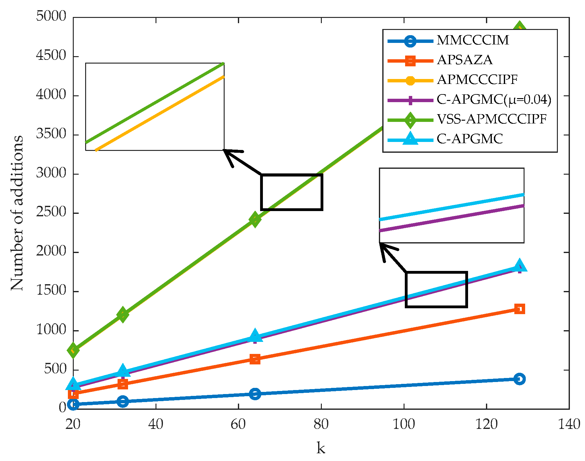
From the above table, it can be concluded that enhancing the adaptability of the algorithm to the environment may come at the cost of increased computational complexity. For example, the algorithm proposed in this paper increases the number of multiplications by 5P + 6 times and the number of additions by P + 20 times after adding the variable-step-size strategy. And after one parameter is determined, a small change in another parameter may also bring a relatively large impact on the complexity of the algorithm, so it is necessary to coordinate the relationship between the projection order of the algorithm and the filter length. In addition, the following figure visualizes the complexity comparison of the algorithms. Since all the affine projection class algorithms used in this paper have a projection order of 4 in the simulation experiments, P = 4 is set to make the length of the unknown system weight vectors k increase sequentially according to the trend of 20, 32, 64, and 128. The Figure 1 and Figure 2 of the change in the number of multiplication and addition operations of several algorithms are obtained, respectively.

From the above charts, it can be seen that the proposed algorithm in this paper has slightly more computation than the MMCCCIM algorithm after adding the CIM paradigm constraints, but the complexity is much lower than that of the same type of APMCCCIPF algorithm because the proposed algorithm does not need to perform matrix inversion. After adding the variable step factor, the complexity of the algorithm increases slightly, since the algorithms in this paper all use diagonal matrices, which actually involve only vector operations, but the computational complexity of the C-APGMC algorithm is still lower than that of the VSS-APMCCCIPF algorithm. In conclusion, all of the above algorithms add sparse regular terms in order to enhance the adaptability to the application scenarios, which increases some computational costs, but the proposed algorithm in this paper has the highest computational efficiency due to the use of the GC-loss scheme instead of the matrix inverse scheme to ensure the accuracy and real-time performance of the signal processing.

6. Simulation Results

In this section, the optimal values of several fixed parameters of the proposed algorithm will be determined and compared with several algorithms of the same type for system identification, and finally, echo cancellation simulation tests will be performed with reference to the above experiments.

The normalized mean square deviation (NMSD) will be employed as a performance metric to evaluate the filtering effectiveness of each algorithm, as defined in Equation (40).

$$\mathrm{NMSD}=10{\log }_{10}\left({\displaystyle \frac{{‖w_0-w\left(n\right)‖}_2^2}{{‖w_0‖}_2^2}}\right)$$

(40)

In the simulation experiments, the steady-state error represents the minimum level of error that the system can achieve after a period of time. Ideally the steady-state error should be close to zero. The lower the value obtained in Equation (40), the closer the steady-state error is to zero. In addition, the speed of convergence of the algorithm can be assessed by observing whether the curve representing the algorithm reaches a steady state of convergence quickly; the steady-state error of the algorithm can be assessed by the lowest value when the curve reaches the steady state; the robustness of the algorithm can be assessed by the degree of fluctuation of the curve under different noise disturbances and whether the curve can converge normally and quickly. The tracking performance of the algorithm can be evaluated by whether the algorithm curve can recover quickly when there is a sudden change in the system impulse response and reach the next steady state, and the steady-state error when each algorithm reaches the fastest convergence will be compared in the experiments as a performance evaluation criterion. The data obtained from the experiments were calculated by averaging the results of 200 independent simulations.

6.1. Algorithm Parameter Selection

The following figure shows the comparison and selection of parameters such as α and kernel width σ in the B(n) matrix of the proposed algorithm. In order to ensure environmental adaptability, we draw on the exhaustive method and grid search method in determining the important parameters. Firstly, we draw on [17,31] to initialize the parameters, and after obtaining the optimal value of the first parameter, we will set it as the initial value to continue to determine the second parameter and so on to obtain the optimal combination of parameters. The simulation experiment environment is the same as the system identification experiment environment. Gaussian white noise has a flat spectral property that can cover all frequency components of the system, and Gaussian noise can be adjusted for its autocorrelation by the autoregressive (AR) model, which enables the input signal to better simulate the statistical properties of the actual signal. Therefore, the input signal used in this system identification experiment is the AR signal, which is obtained from the Gaussian white noise signal trained by the AR training model:

$$G\left(z\right)={\displaystyle \frac{1+0.5z^{-1}+0.81z^{-2}}{1-0.59z^{-1}+0.4z^{-2}}}$$

(41)

where z is a complex variable that characterizes the signal in the frequency domain. G(z) represents the transfer function of the autoregressive model, describing the relationship between the input and output signals. The model is trained with a Gaussian white noise signal, which serves as the input. This approach enhances the adaptive filter’s recognition accuracy and improves convergence speed.

The algorithms in the experiments are projected with order P = 4. The unknown system is randomly generated from numbers between −1 and 1 according to the set sparsity with a length of 120. The total number of iterations for the algorithm in the non-smooth environment is 2 × 10⁴, where the system impulse response changes from w₀ to −w₀ at 1 × 10⁴ iterations. The Gaussian noise signal-to-noise ratio is 20 dB throughout the system identification simulation experiments. In the experiment each parameter will be taken from small to large within a reasonable range. Based on the experimental outcomes, the point with the lowest steady-state error, while maintaining the same convergence rate, is selected as the optimal value for use in subsequent experiments.

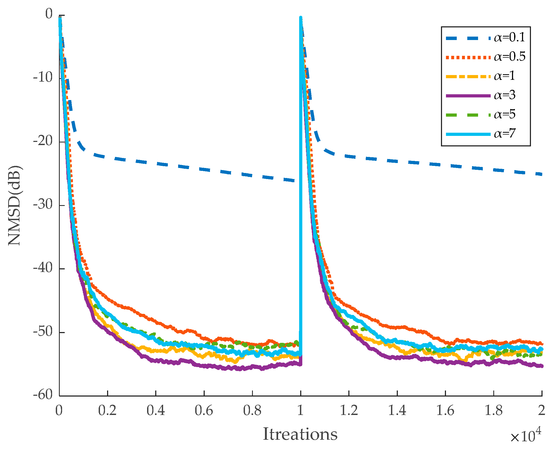
It should be noted that the parameter sensitivity analysis range of this experiment is determined based on a large number of simulation experiments, and parameter selection outside the range is likely to cause the algorithm to fail to converge properly. Therefore, in order to ensure that the algorithm can operate efficiently and stably in the real environment, the impact of parameter selection on the performance of the algorithm will be analyzed in depth within the current range. For parameter α, too large a value can lead to too much influence of the error on the algorithm, and too small a value can weaken the adaptive performance of the algorithm. 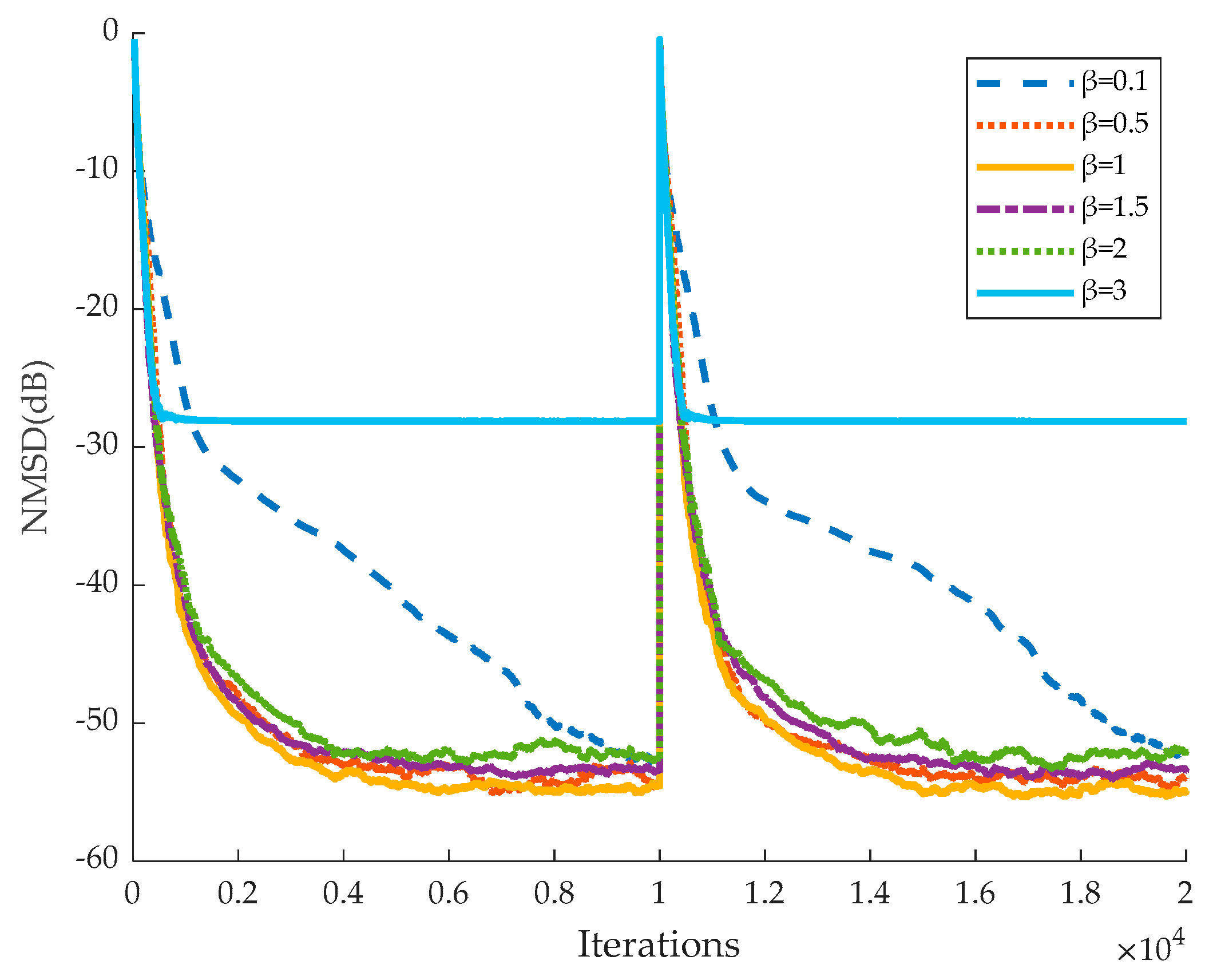For parameter β, too large a value will result in the algorithm relying too much on the sparsity of the system, and too small a value will weaken the algorithm’s ability to adapt to sparse systems. 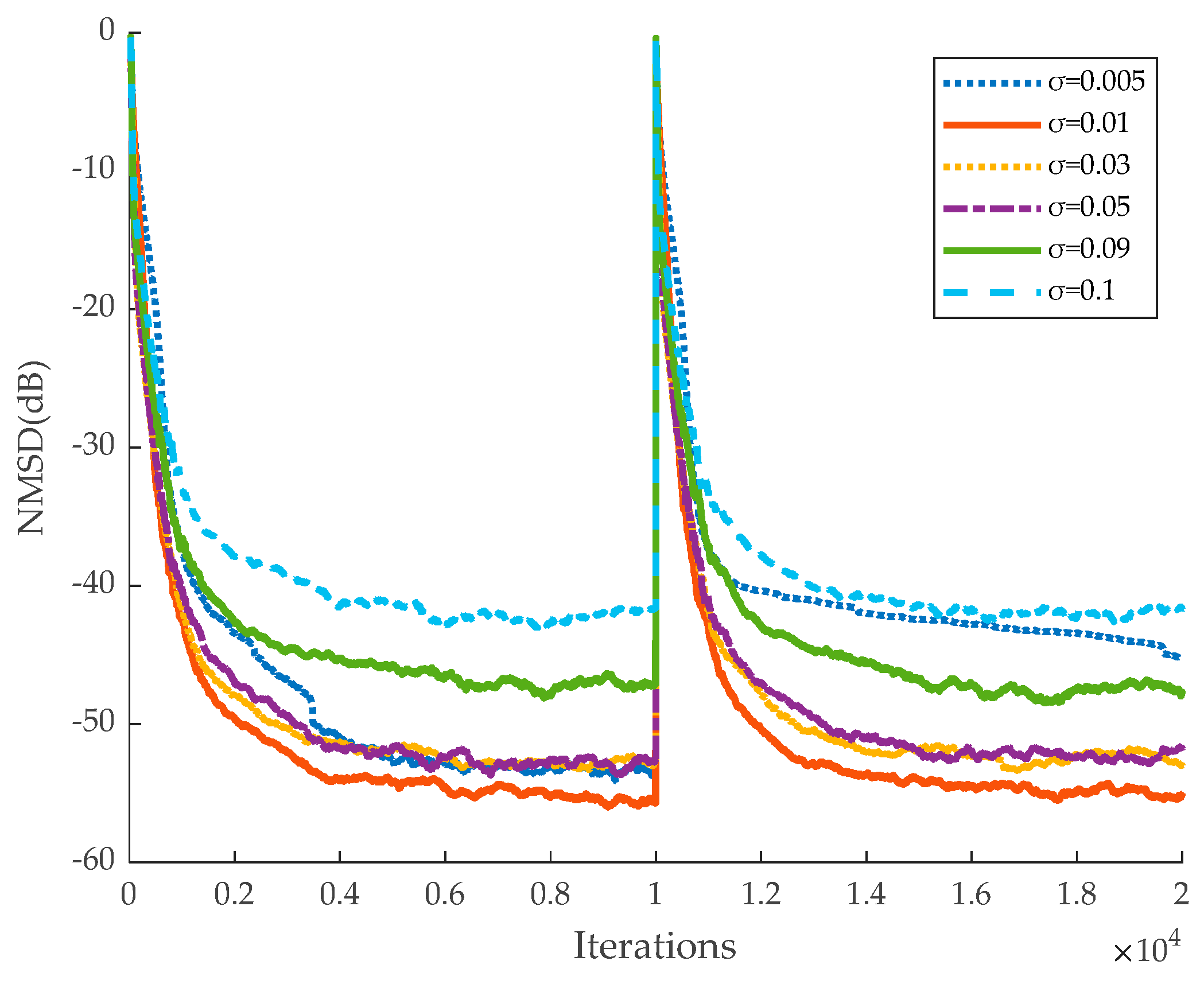For the parameter σ, a value that is too large may hinder the algorithm’s ability to adapt to complex signal dynamics, while a value that is too small could lead to overfitting. Regarding the parameter t, an excessively large value causes the algorithm to overly depend on past data, slowing down convergence. Conversely, a value that is too small results in rapid changes in the step size, reducing the algorithm’s stability. As shown in Figure 3, when the parameter α in the matrix B(n) is within the range of (0.5, 7), the algorithm achieves faster convergence and a lower steady-state error. When α is less than 0.5, the algorithm exhibits a high steady-state error and fails to converge after 1 × 10⁴ iterations. Furthermore, when α exceeds 3, the steady-state error increases as α rises. Based on these observations, the optimal value of α for the algorithm is determined to be 3. Similarly, as shown in Figure 4, Figure 5 and Figure 6 the best parameters are identified as β = 1, σ = 0.01, and t = 0.997.

6.2. Sparse System Identification

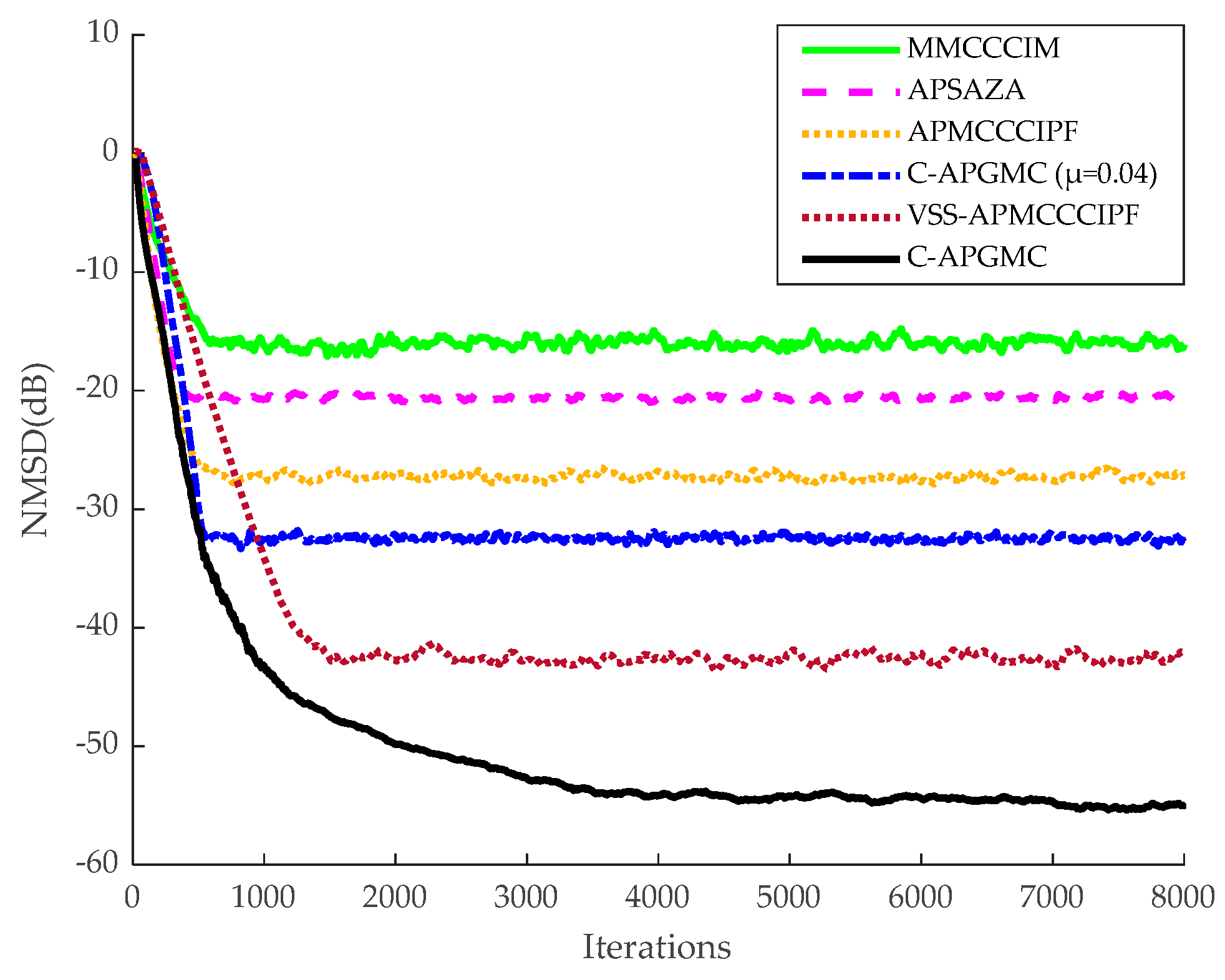
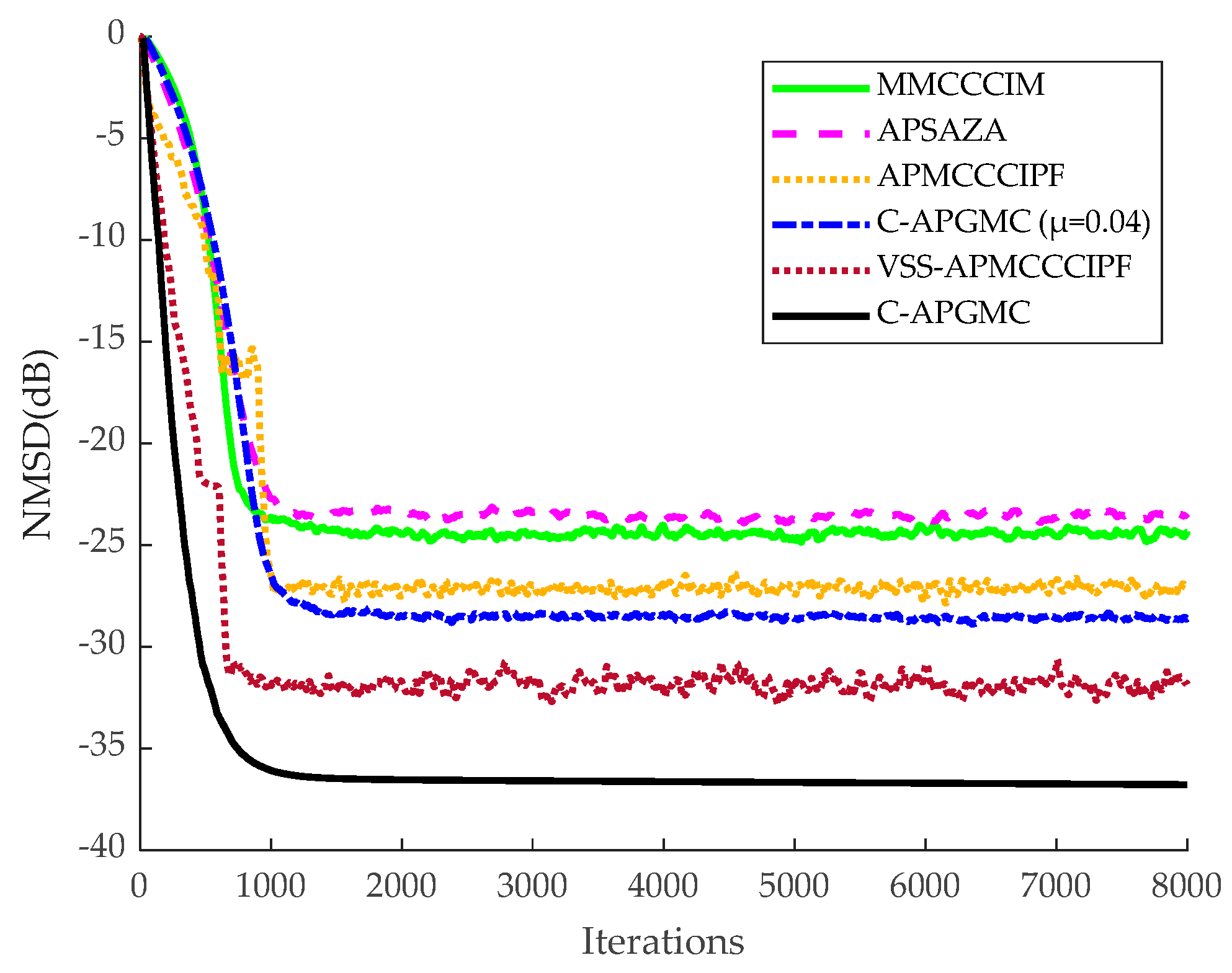
Before the echo cancellation simulation, a system identification simulation experiment needs to be set up in order to provide reasonable initial parameter settings for the adaptive filters so that the individual filter algorithms can achieve the fastest convergence rate. In this section, the algorithm proposed in this paper is compared with the same type of MMCCCIM, APSAZA, APMCCCIPF, and VSS-APMCCCIPF algorithms, and in order to enhance the comparison of the effects, the fixed-step version of the algorithm proposed in this paper is also included in the comparison.

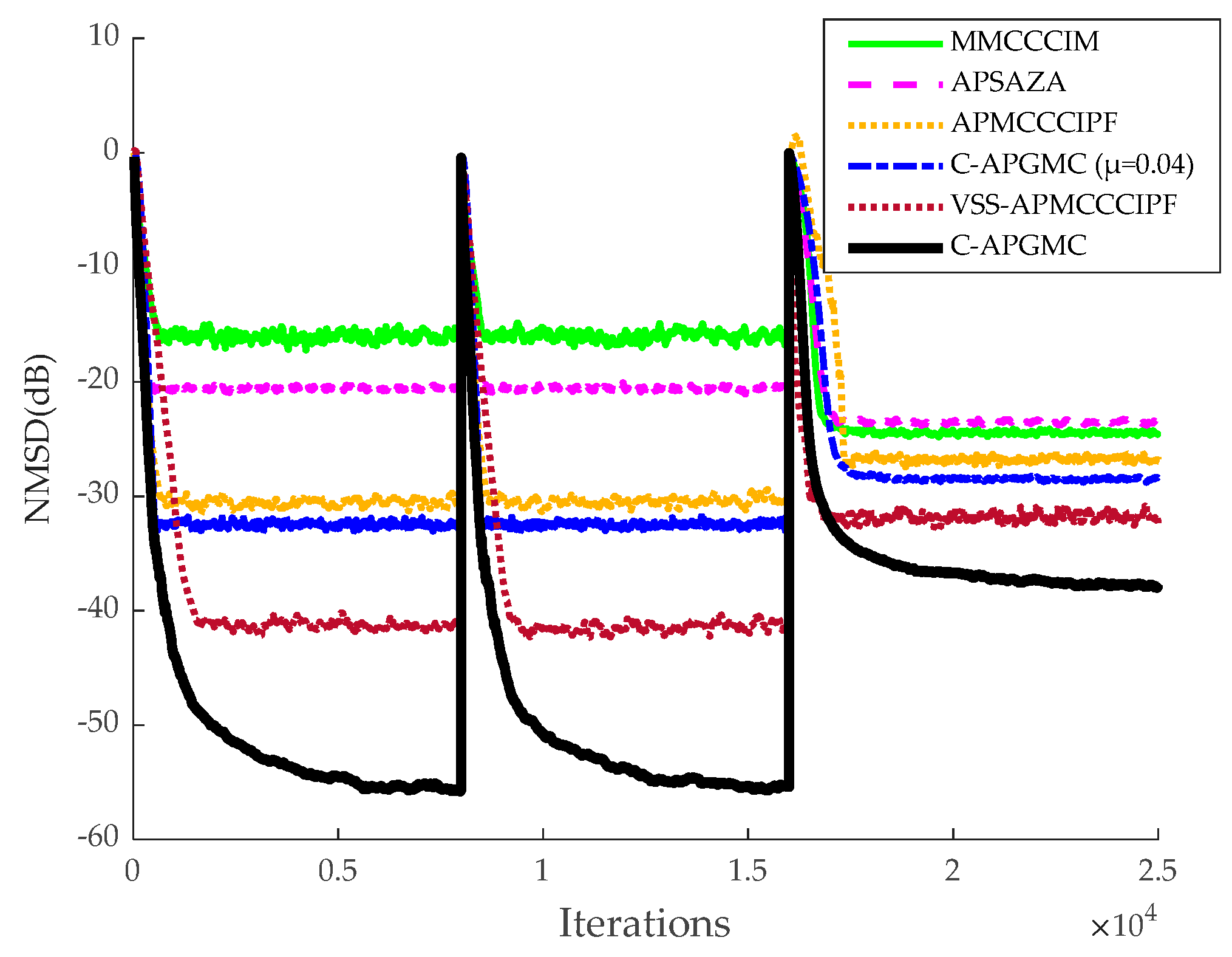
The number of iterations in this experiment was 8000 in the smooth environment and 2.5 × 10⁴ in the non-smooth environment. To ensure that the performance of each algorithm is optimal, the step size is set to μ = 0.08 for the MMCCCIM algorithm, μ = 0.02 for the APSAZA algorithm, μ = 0.04 for the APMCCCIPF algorithm, the kernel width σ = 0.01, and the zero-attraction factor β = 0.0001. For the VSS-APMCCCIPF algorithm, the step size of the variable parameter in the convex combination factor t = 0.98. For the C-APGMC algorithm, α = 3, β = 1, kernel width σ = 0.01, the convex combination factor t = 0.997. The results are shown in the Figure 7, Figure 8 and Figure 9.

As can be seen from the above figures, in the sparse system, the MMCCCIM algorithm has the worst effect because it does not reuse the input signal. In addition, compared with CIM, which approximates l₀-paradigm, the APSAZA algorithm performs poorly due to the fact that it employs l₁-paradigm as a sparse penalty term, and its zero-attraction ability is weaker than that of CIM [24]. The APMCCCIPF algorithm and the proposed algorithm have better performance due to the combination of faster convergence of the AP algorithm and advanced sparse constraints, and the APMCCCIPF algorithm has simpler structure due to sparse constraints on the CIPF function in order to reduce the complexity and its steady-state error is slightly higher than the fixed-step version of the algorithm proposed in this paper. The VSS-APMCCCIPF algorithm adopts a variable-step strategy and its steady-state error is further reduced compared with the fixed-step version of the algorithm proposed in this paper. In comparison, the C-APGMC algorithm presented in this study, which employs the MSD method to derive a variable-step-size formula and incorporates historical input signals, demonstrates superior performance in both convergence speed and steady-state error. In non-sparse systems, the algorithm proposed in this paper still has the smallest steady-state error, and in this experiment, it can be seen that the algorithm proposed in this paper can also perform well if there are multipath echo channels in the echo cancellation scenario of the algorithm, which results in a decrease in the sparsity of the echo paths. The above experiment confirms the effectiveness of the C-APGMC algorithm and its variable-step-size strategy proposed in this paper in the application of system identification scenarios.

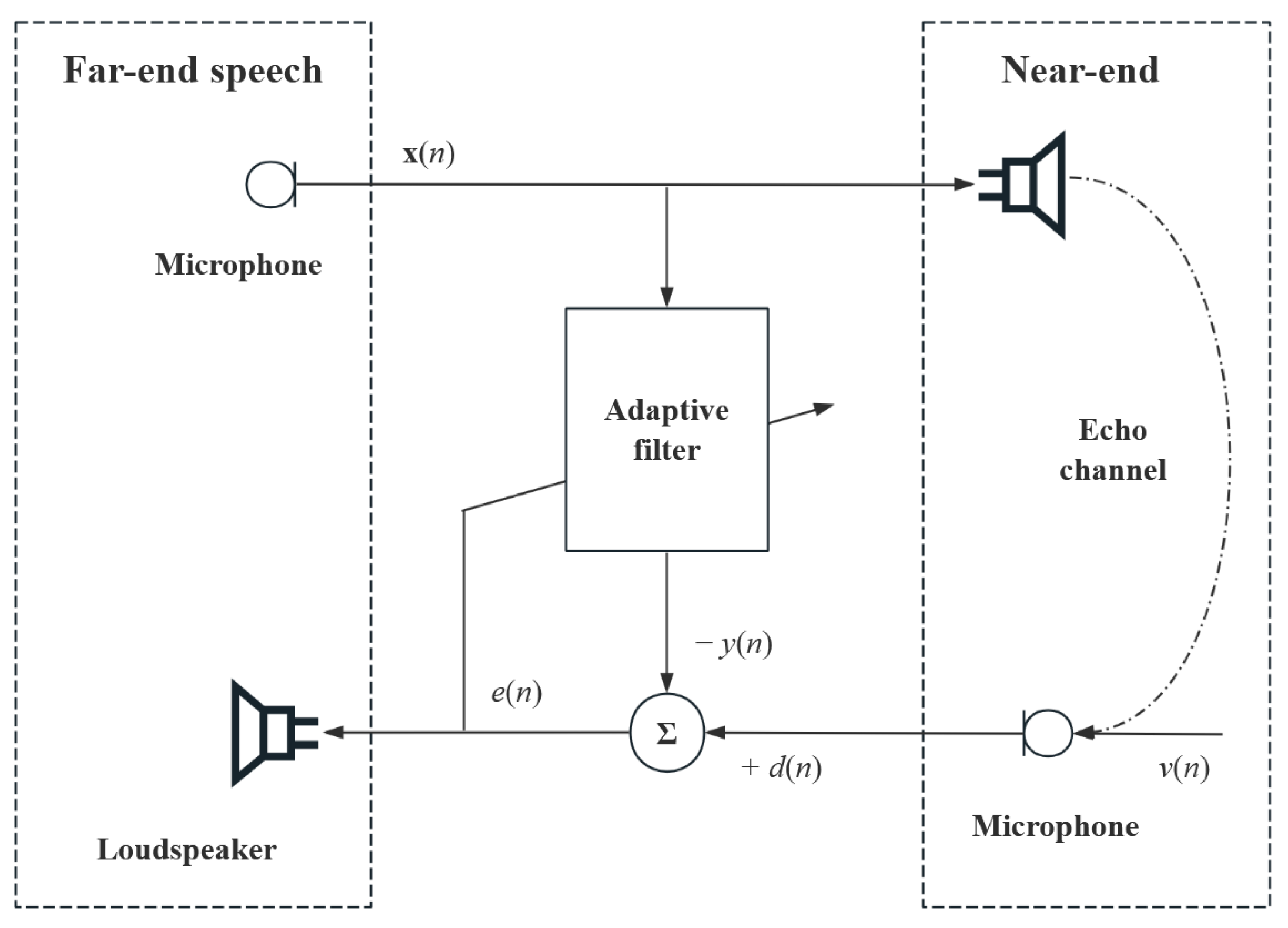
6.3. Echo Cancellation

This section continues to validate the performance of the proposed algorithm in echo cancellation scenarios. As shown in the Figure 10, the speech signal x(n) from the far end is transmitted to the near end, undergoes various reflections, is interspersed with noise v(n) to form an echo signal d(n) that is collected by the directional microphone, and is finally re-transmitted back to the far end. It should be noted that the movement of the near-end microphone position will cause an abrupt change in the impulse response of the echo system. The adaptive algorithm will simulate the echo path through known conditions to obtain a more accurate echo signal, thus eliminating the echo.

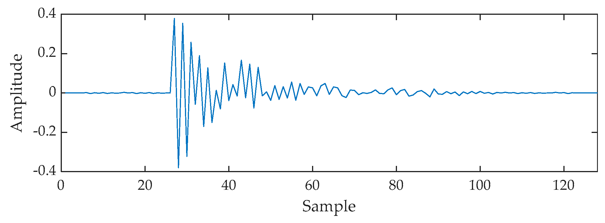
By analyzing the results of the sparse system identification experiments, setting the system impulse response length to 128 better reflects the indoor characteristics of the echo cancellation scenario, and the algorithm can exert its maximum performance under the echo path of this length. The echo cancellation simulation experiments in this paper are all performed with the same system impulse response and this sparse path setting is shown in the Figure 11:

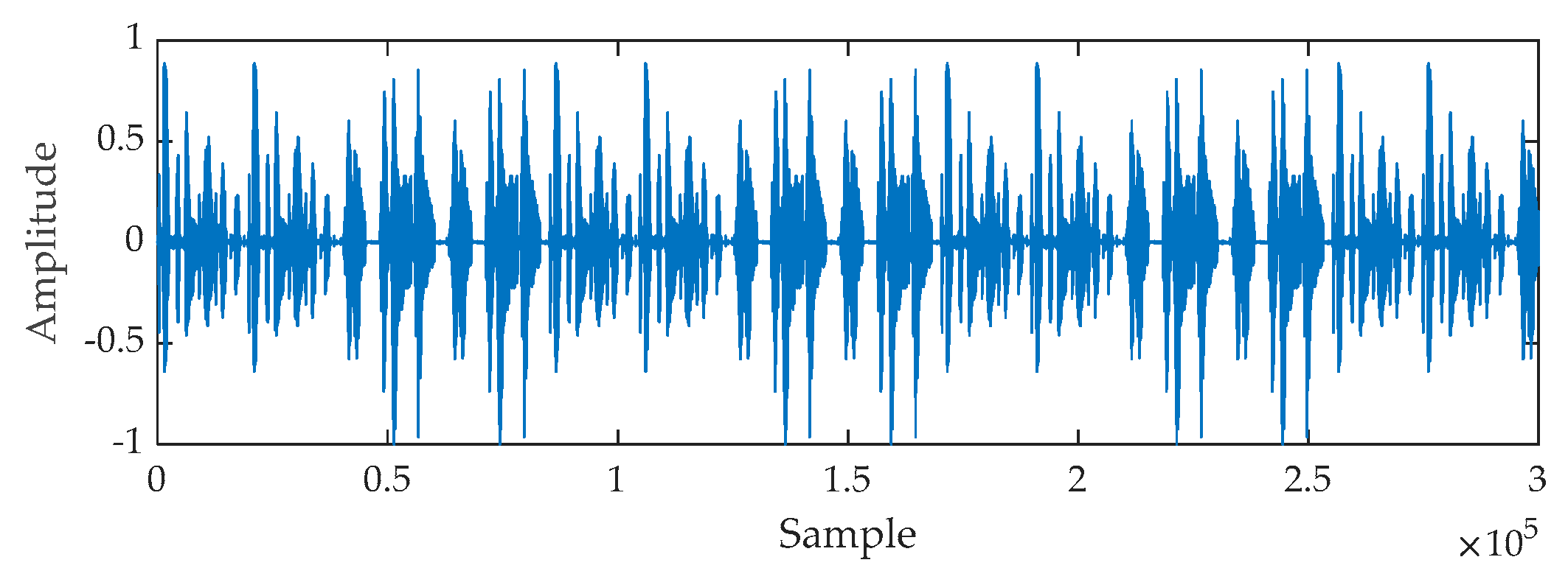
In the above figure, most of the impulse response values are zero or very small, with a peak only at a sample length of 27, which decays with time, which is consistent with the characteristics of non-multipath echo channels and delayed propagation in indoor teleconferencing and is suitable for modeling this scenario. The input signal is a real speech signal with a sampling frequency of 8 kHz and its waveform is shown in the Figure 12.

To ensure the optimal performance of each algorithm, for the APMCCCIPF algorithm, the step size is set to μ = 0.04, the kernel width σ = 0.1, the zero-attraction factor β = 1 × 10⁻⁶, and the rest of the algorithmic parameter settings are the same as those used in the above-mentioned system identification applications. To assess the performance of each algorithm under varying noise conditions, the final set of simulation experiments includes Gaussian noise with a signal-to-noise ratio of 20 dB, as well as impulsive noise following an α-stable distribution [38]. 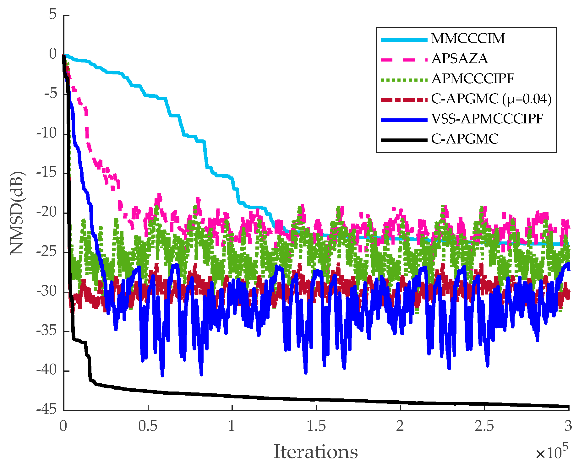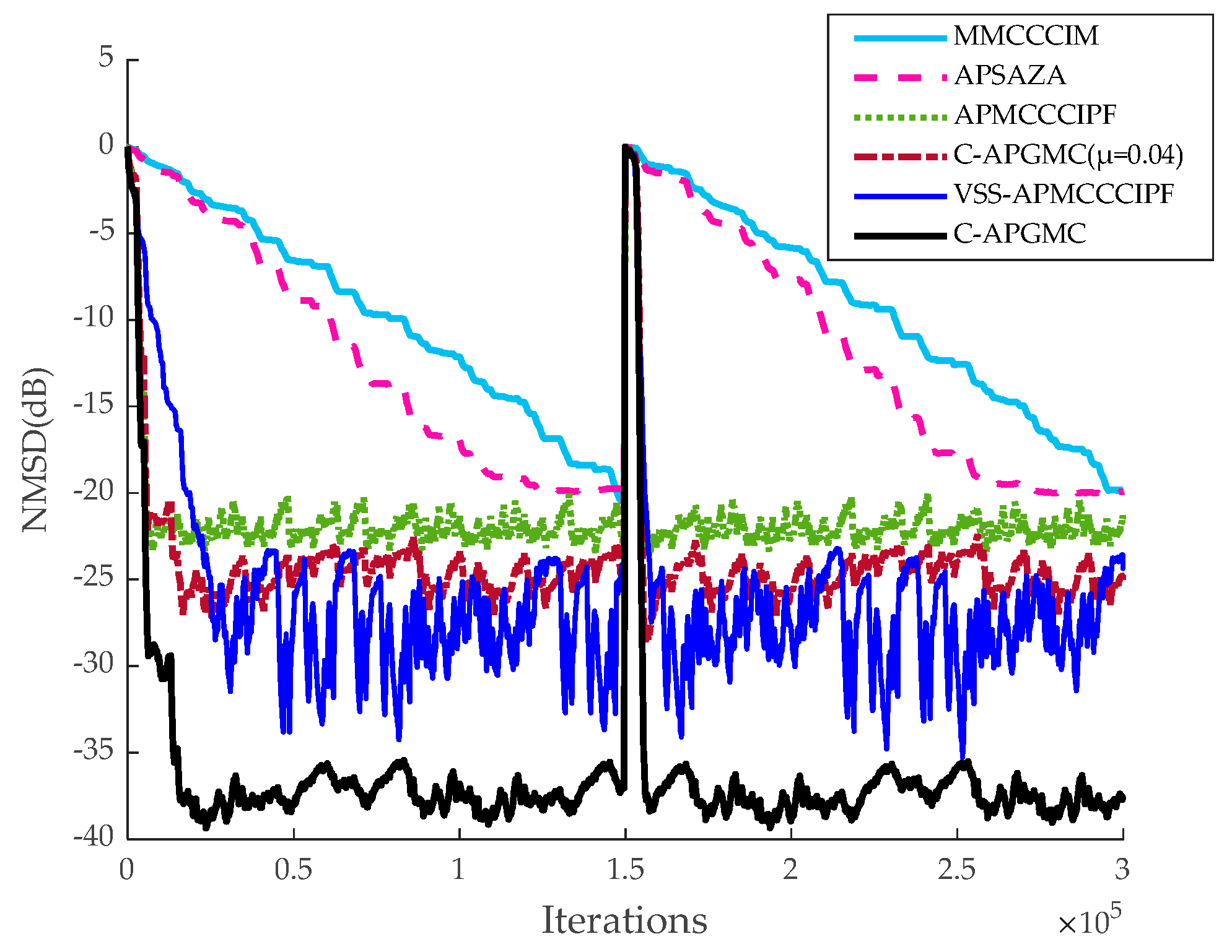The Figure 13, Figure 14 and Figure 15 present the simulation outcomes for all six algorithms across different echo cancellation scenarios.

The above comparison shows that with approximately the same convergence rate for all types of algorithms, the steady-state error of the C-APGMC algorithm with fixed step size is between those of the APMCCCIPF algorithm and the VSS-APMCCCIPF algorithm, and C-APGMC has the smoothest performance in reaching the steady state with the smallest steady-state error due to the availability of convex combination factors. Upon introducing mixed noise, the performance of all algorithms is impacted to some degree. However, the algorithm presented in this study maintains low steady-state error and high stability, thanks to the aforementioned advantages. The above results demonstrate the strong performance of the algorithm proposed in this paper in the simulation of indoor sparse echo channels compared to other algorithms of the same type, proving that the algorithm possesses a relatively strong echo cancellation effect in indoor teleconferencing scenarios.

7. Conclusions

This paper proposes the C-APGMC algorithm, which is based on the generalized maximum correlation entropy affine projection (APGMC) algorithm. The algorithm uses the CIM method as a sparse penalty term, making it more suitable for application scenarios such as echo cancellation. In addition, a variable-step-size formulation of the algorithm is derived by means of the MSD method and the introduction of a convex combinatorial factor. The performance analysis and simulation results show that, although the introduction of a variable step factor slightly increases complexity, the algorithm achieves faster convergence, reduced steady-state error, and improved tracking capability in sparse systems. Additionally, the proposed algorithm outperforms recent methods, such as the APMCCCIPF algorithm, which are also designed for sparse systems. Finally, from the comparative simulation experiments of echo cancellation with different noise inputs, it can be concluded that the interference of strong impulse noise is not conducive to the performance of the proposed algorithm in sparse echo path recognition, and the present algorithm is more suitable for indoor echo cancellation environments. Future research could try to incorporate active noise control (ANC) techniques to reduce the effect of strong impulse noise on echo cancellation algorithms.