Abstract
To maintain product reliability and stabilize performance, it is essential to prioritize the identification and resolution of latent defects. Advanced products such as high-precision electronic devices and semiconductors are susceptible to performance degradation over time due to environmental factors and electrical stress. However, conventional performance testing methods typically evaluate products based solely on predefined acceptable ranges, making it difficult to predict long-term degradation, even for products that pass initial testing. In particular, products exhibiting borderline values close to the threshold during initial inspections are at a higher risk of exceeding permissible limits as time progresses. Therefore, to ensure long-term product stability and quality, a novel approach is required that enables the early prediction of potential defects based on test data. In this context, the present study proposes a machine learning-based framework for predicting latent defects in products that are initially classified as normal. Specifically, we introduce the Sigma Deviation Count Labeling (SDCL) method, which utilizes a Gaussian distribution-based approach. This method involves preprocessing the dataset consisting of initially passed test samples by removing redundant features and handling missing values, thereby constructing a more robust input for defect prediction models. Subsequently, outlier counting and labeling are performed based on statistical thresholds defined by 2σ and 3σ, which represent potential anomalies outside the critical boundaries. This process enables the identification of statistically significant outliers, which are then used for training machine learning models. The experiments were conducted using two distinct datasets. Although both datasets share fundamental information such as time, user data, and temperature, they differ in the specific characteristics of the test parameters. By utilizing these two distinct test datasets, the proposed method aims to validate its general applicability as a Predictive Anomaly Testing (PAT) approach. Experimental results demonstrate that most models achieved high accuracy and geometric mean (GM) at the 3σ level, with maximum values of 1.0 for both metrics. Among the tested models, the Support Vector Machine (SVM) exhibited the most stable classification performance. Moreover, the consistency of results across different models further supports the robustness of the proposed method. These findings suggest that the SDCL-based PAT approach is not only stable but also highly adaptable across various datasets and testing environments. Ultimately, the proposed framework offers a promising solution for enhancing product quality and reliability by enabling the early detection and prevention of latent defects.
1. Introduction
Early detection and mitigation of latent defects play a critical role in maintaining stable product performance. High precision electronic devices, such as semiconductors, may exhibit performance degradation or failures under actual operating conditions, even if they have successfully passed initial product testing [1]. Conventional performance evaluation methods classify products as normal as long as the test results fall within predefined thresholds. However, products that exhibit results near the boundary values may initially be deemed acceptable but can drift beyond allowable limits over time [2,3]. The causes of such latent defects are diverse and include inter cell interference caused by semiconductor miniaturization, inherent limitations in inspection processes, and the emergence of new types of defects [4]. These factors can lead to increased warranty costs, reduced product reliability, and damage to the company’s reputation. In severe cases, latent defects in semiconductors may even pose safety risks to end users [5]. Therefore, to ensure the long-term performance and reliability of products, a predictive approach is required one that can identify devices likely to experience future degradation based on their initial test results [6].
Traditionally, latent defects have been detected through post manufacturing screening processes such as burn-in testing and Environmental Stress Screening (ESS) [7]. These methods are primarily designed to eliminate early life failures referred to as infant mortality which tend to cluster in the initial phase of the failure rate curve, commonly known as the bathtub curve [8]. By subjecting products to elevated levels of stress, including high temperature and voltage, these procedures aim to identify and eliminate defective units prior to deployment [8]. However, such screening techniques are often costly and time consuming [8]. Furthermore, it is challenging to replicate all possible stress conditions that a product may encounter in the field. In modern manufacturing environments, the emergence of novel failure mechanisms makes it increasingly difficult for traditional methods to effectively capture all latent defects [9]. These limitations highlight the growing need for data driven approaches in defect detection and reliability assurance. In response to these challenges, the industry has increasingly adopted the Part Average Test (PAT) as a complementary strategy to reduce dependency on burn-in testing while improving early defect detection accuracy [10]. Static and dynamic Part Average Testing (PAT) techniques are statistical test methodologies employed in semiconductor manufacturing processes to facilitate early identification of latent defects [11]. Static PAT establishes test limits based on data from previously tested lots, whereas dynamic PAT calculates these limits using data derived from the current lot under evaluation. However, conventional PAT methods exhibit inherent limitations in effectively capturing subtle anomaly signals or minor process variations. Static PAT is limited in its responsiveness to real time changes in process conditions, while dynamic PAT tends to be vulnerable to noise and variability introduced during data collection and analysis [12].
To overcome the limitations of traditional statistics-based methods and improve predictive accuracy, recent research has increasingly focused on data driven approaches utilizing machine learning and deep learning techniques for latent defect prediction. Wang and Yang proposed a machine learning-based analysis method to address random defects arising from equipment variability, analyzing the impact of equipment combinations on production yield [13]. Their method was applied to a real-world DRAM manufacturing plant, where it successfully identified abnormal equipment combinations and enabled process engineers to take prompt corrective actions. Kim and Joe introduced a framework aimed at identifying root cause processes responsible for rare latent defects. By generating virtual bad wafers and employing large scale data processing techniques, they significantly improved both the accuracy of defect source identification and the speed of analysis [4]. P. Lenhard et al. presented a die level predictive modeling approach utilizing inline defect inspection data collected during semiconductor manufacturing processes [10]. By combining saliency map clustering with advanced predictive engines, their method was able to identify dies with latent reliability risks that had passed wafer sort, thereby reducing defect escapes in post packaging stages and enhancing overall product reliability. Hu et al. proposed an unsupervised anomaly detection algorithm based on machine learning to identify and eliminate rare defective semiconductor devices that have passed standard testing procedures. The method employs a self-labeling technique in which normal data are transformed using power, Chebyshev, and Legendre polynomials to generate unique labels. This transformation process facilitates the training of a classifier capable of learning hidden patterns within the normal dataset, thereby enabling effective identification of latent defects that exhibit subtle behavioral deviations from normal chips [14].
This study proposes a post process prediction method aimed at mitigating the high cost and time loss associated with traditional screening techniques, by enabling the detection of latent defects prior to the execution of screening tests. The proposed Sigma Deviation Count Labeling (SDCL) method assigns labels to statistically defined outliers and leverages these labels within a supervised machine learning framework for defect prediction. By identifying and filtering out products with a high likelihood of performance degradation despite having passed initial tests as normal the proposed method enables significant savings in terms of cost, labor, and time typically incurred by subsequent screening procedures. Furthermore, by ensuring that only products with stable performance are shipped, the approach contributes to improved long-term quality management and enhanced product reliability. While the study by Hu et al. [14] shares the common objective of detecting latent defects at an early stage prior to product shipment, as well as the utilization of data from devices that have passed standard testing, several distinctions exist in terms of learning methodology and interpretability. Hu et al. adopt an unsupervised learning approach based on self-labeling to identify anomalies, whereas the present study assigns weak labels to statistically defined outliers and employs a supervised learning framework for model training. From an interpretability standpoint, Hu et al.’s method demonstrates strengths in representation learning and anomaly scoring, whereas the proposed approach leverages an intuitive feature namely, anomaly count to facilitate the identification of defective variables or specific process segments. Furthermore, due to its simplicity in parameter tuning, the proposed method can be readily adapted to sudden environmental changes in real-world manufacturing settings through rapid adjustment of threshold values
2. Related Work
In this study, the proposed SDCL method is compared with two widely used statistical outlier detection approaches in order to extract anomalies from normal datasets and enable subsequent machine learning training. For this purpose, the Median Absolute Deviation (MAD) method and the Interquartile Range (IQR) method were selected as benchmarks for comparison.
2.1. Outlier Detection Based on the Normal Distribution
Assuming that the data follows a normal distribution, the majority of observations are concentrated within a specific range around the mean. The spread of this distribution is determined by the standard deviation (σ), and it is well established that the probabilities of data falling within ±1σ, ±2σ, and ±3σ are 68.27%, 95.45%, and 99.73%, respectively [15]. Based on these statistical properties, thresholds can be defined in terms of σ, whereby observations exceeding these limits are regarded as statistical outliers [16]. Table 1 presents the proportions of data located inside and outside each sigma range. Outlier detection techniques based on the assumption of a Gaussian distribution inherently rely on the premise that the underlying data follows a normal distribution. However, in cases where the actual data distribution is asymmetric, this assumption is violated, increasing the likelihood of false detections. Moreover, both the mean and standard deviation are highly sensitive to extreme values the presence of even a small number of outliers can lead to inflated standard deviation estimates. When the dataset is small, the uncertainty in estimating σ becomes more pronounced, potentially resulting in biased threshold settings. Consequently, the relaxation of detection boundaries may hinder the effective identification of latent anomalies [17].

Table 1.
Probability Distribution by Sigma.
2.2. Mean Absolute Deviation
The MAD measures the extent to which each observation deviates from the median of a dataset in absolute terms and subsequently computes the median of these absolute deviations [7]. The MAD is formally defined as shown in Equations (1) and (2).
X is a set of observations. When the observations are assumed to follow a normal distribution, a correction factor of is applied. The parameter denotes a user defined sensitivity adjustment factor, which is commonly set to . Although this method has been reported in previous studies to yield effective results in outlier detection, its reliability decreases when more than 50% of the dataset consists of outliers, as the median itself may become distorted, thereby reducing the robustness of MAD [16]. However, the MAD also has limitations, particularly in small datasets, where the variability of the estimate increases and the robustness of both the median and absolute deviation diminishes. This issue becomes especially pronounced when the data exhibits strong skewness or complex clustering structures, in which case the median may fail to adequately represent the center of the overall distribution, leading to distorted outlier detection. Furthermore, since MAD is based on deviations from the median, it is relatively insensitive to subtle shifts in the central tendency of the distribution. As a result, when extreme values are prevalent, the sensitivity of outlier detection may be significantly reduced [18].
2.3. The Interquartile Range
The IQR is defined as the difference between the third quartile (Q3) and the first quartile (Q1) of a dataset, and it is calculated according to Equations (3) and (4) [19].
In the IQR method, the threshold is determined by multiplying the interquartile range by 1.5. Specifically, the lower bound is defined as while the upper bound is defined as Any observations falling outside this range are classified as outliers. However, a limitation of this approach is that extreme outliers can influence the values of or , thereby distorting the threshold calculation itself [20]. However, the IQR method also presents several limitations. First, when the data distribution is highly skewed or contains a large number of extreme values, the actual variability may be over or underestimated, leading to distorted outlier detection boundaries. Second, in the case of small sample sizes, quantile estimates may become unreliable and yield inaccurate thresholds. Third, similar to the aforementioned methods, IQR does not account for the structural characteristics of multimodal distributions, making it less effective in detecting outliers when multiple clusters are present [8,21].
3. Data Set
The datasets used in this study were provided by StatsChippackKorea (SCK) and consist of two distinct sets: a primary dataset and a secondary dataset, both derived from products that initially passed defect screening tests. The primary dataset contains a total of 14,140 samples, each described by 1804 features including timestamp, user information, temperature, and signal values. Due to the variability of test items across different products in actual manufacturing processes, the secondary dataset was constructed with different test features in order to evaluate the robustness and generalizability of the proposed model. Specifically, it is designed to verify whether the model trained on the primary dataset can maintain stable performance when applied to a dataset with altered test conditions. The secondary dataset comprises 80,819 samples, sharing common basic information such as time, user data, and temperature with the primary dataset, but differing in test related features. It includes a total of 454 features.
4. Data Preprocessing
In this study, the preprocessing procedure for latent defect detection using machine learning is illustrated in Figure 1. The process begins with data cleaning, in which missing values and irrelevant features for model training are removed from the normal dataset. Subsequently, in the outlier counting step, the number of anomalies for each sample is calculated across individual features based on the normal distribution, and this count is introduced as a new feature. Finally, the computed outlier counts are re-evaluated using the same normal distribution–based outlier detection method, through which products are relabeled as either normal or abnormal.
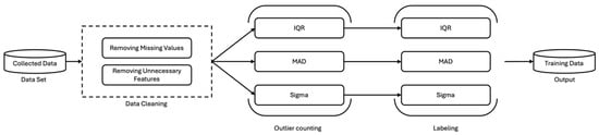
Figure 1.
Data preprocessing procedures for potential flaws in a normal dataset.
Since the assumption of normality may not always hold, this study applied not only the normal distribution–based method but also the median-based MAD approach and the quartile-based IQR method during the threshold setting and labeling processes. These additional methods were incorporated to enable comparative analysis. Through this design, the performance of each outlier detection technique can be evaluated across datasets exhibiting different distributional characteristics.
4.1. Data Cleaning
During the data collection phase, missing values may arise due to a variety of technical and environmental factors, such as sensor malfunctions, network latency, and external fluctuations [22]. These missing values can distort the distribution of the training data, potentially degrading prediction performance or, in extreme cases, rendering model training infeasible. As such, data cleaning becomes an essential preprocessing step. Common strategies for handling missing data include deletion, simple imputation, and the use of predictive models. However, deletion methods may introduce bias due to the loss of sample size and the potential elimination of meaningful patterns. Predictive modeling approaches, while more sophisticated, may result in biased estimations or overfitting if the models used for imputation are poorly trained [23]. Simple imputation techniques also carry the risk of compromising the data’s variance and covariance structure, thereby weakening the model’s generalization capability [24]. In this study, variables containing missing values were removed without applying dimensionality reduction or complex feature selection procedures, with priority given to maintaining data quality. Furthermore, variables composed of constant values or those lacking informative variability such as user identification fields were excluded, as they were deemed irrelevant for meaningful model training [25].
As a result of this preprocessing step, the number of features in the 1st dataset was reduced from 1804 to 1664, while the 2nd dataset was reduced from 454 to 374 features. The overall number of samples and features for each dataset is summarized in Table 2.
Table 2.
Characteristics and data counts of the different datasets provided by SCK.
4.2. Outiler Count and Labeling
As a method for latent defect prediction, a statistical outlier detection approach based on standard deviation thresholding is applied. With input from domain experts, thresholds are defined using the ±2σ and ±3σ ranges, and the number of features in each sample that exceed these threshold boundaries is counted. Figure 2 illustrates the results of outlier counting in the first dataset under the ±2σ and ±3σ criteria. The majority of samples are concentrated around relatively low outlier counts, indicating that most observations fall within the normal range. In contrast, a subset of samples exhibits comparatively high outlier counts and is located in the tail regions of the distribution. Such samples correspond to statistical outliers, lying outside the distributional boundaries, and may therefore represent potential risk factors or early signs of abnormality.
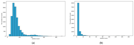
Figure 2.
(a) Histogram of Outlier Counts Using 2σ Rule on First Dataset (b) Histogram of Outlier Counts Using 3σ Rule on First Dataset.
Defined in addition, to account for cases where the data do not follow a normal distribution, outlier detection methods based on MAD and IQR were also employed. These two approaches are advantageous in that they are less sensitive to extreme values and are effective for non-normally distributed datasets [15,16]. For the MAD method, the threshold was set according to the commonly used criterion of , while for the IQR method, the threshold was defined as The subsequent labeling process was performed using the same detection methods and thresholds applied during the outlier counting stage, with final outlier designations determined based on the precomputed counts. For example, when outlier counting was conducted using the ±2σ criterion, labeling was likewise assigned according to the number of outliers identified under the ±2σ threshold. Table 3 summarizes the processes and labeling outcomes for each outlier detection method, along with their respective proportions.
Table 3.
Clustering Results of 1st and 2nd Datasets Based on σ Thresholds.
5. Performance Results
In this study, the 1st and 2nd datasets were utilized to perform outlier detection based on Sigma, IQR, and MAD methods. These detection techniques were further combined with various scaling approaches (None, Normalization, Min–Max scaling, and Standardization) and machine learning models, including Logistic Regression, Support Vector Machine, Extreme Gradient Boosting, Adaptive Boosting, Decision Tree, and K-Nearest Neighbors. The selection of models in this study is supported by prior research demonstrating their effectiveness on similar datasets. In the case of Logistic Regression (LR), Jizat et al. reported a classification accuracy of approximately 86.9% in wafer defect classification, outperforming Support Vector Machines (SVM) and k-Nearest Neighbors (k-NN) under identical experimental conditions [26]. SVM achieved a maximum accuracy of around 70–72% in a study by Hu et al., which applied an optimized Radial Basis Function kernel and feature selection techniques to high-dimensional semiconductor process data [27]. XGBoost 3.0.5 demonstrated outstanding performance in Taha’s wafer defect pattern classification experiment, achieving approximately 94.8% accuracy and an F1-score of 92.6%, while maintaining a relatively short training time compared to traditional classifiers [28]. In addition, AdaBoost, Decision Tree (DT), and k-NN models also showed competitive predictive accuracy reporting RMSE values ranging from 0.65 to 0.71 alongside Random Forest in the wafer yield prediction study by Lee and Roh [29]. These previous findings collectively support the suitability and competitiveness of the models adopted in this study, particularly in handling high dimensional datasets. To effectively evaluate the trade-off between sensitivity and specificity in the test results, Geometric Mean (GM) [30] and accuracy are adopted as the primary performance metrics. Sensitivity and specificity, which are required for GM calculation, are defined as shown in Equations (5) and (6), respectively [31]. These metrics are computed based on the confusion matrix elements: True Positive (TP), True Negative (TN), False Positive (FP), and False Negative (FN). Specifically, TP refers to correctly predicted positive cases, TN to correctly predicted negative cases, while FP and FN represent incorrectly predicted positive and negative cases, respectively. By applying these definitions, the model’s ability to accurately predict both positive and negative instances can be quantitatively assessed. The final GM is then computed as shown in Equation (7). objective is to predict latent defective products, the evaluation emphasizes balanced performance between normal and potentially defective samples. Therefore, the final experimental results are reported based on the top performing model combination, selected according to the highest GM achieved by each model.
Table 4 presents the results obtained for Process 1 and Process 2 when both outlier counting and labeling were conducted using the MAD method. A comparative analysis of the GM values across the two datasets indicates that, for most models, Process 2 exhibits a decline in GM relative to Process 1. Notably, the KNN model demonstrated the largest decrease, with GM dropping from 88.2% in Process 1 to 75.5% in Process 2, representing a reduction of 12.7pp. By contrast, the other models showed smaller declines ranging from 1.4 to 3.8% producing relatively consistent outcomes. These findings suggest that, with the exception of KNN, the models were able to achieve stable detection performance using the MAD-based approach.
Table 4.
Results of Processes 1 and 2 Using MAD 1.
Table 5 presents the results obtained for Process 3 and Process 4 when both outlier counting and labeling were conducted using the IQR method. Compared with Process 3, Process 4 demonstrates either an improvement or maintenance of GM performance. In particular, the SVM, XGB, and LR models exhibit increases in GM of 8.8, 6.1, and 3.5pp, respectively. These results indicate that, despite Process 4 having fewer features, stable detection performance can still be achieved.
Table 5.
Results of Processes 1 and 2 Using IQR 1.
Table 6 presents the results for Processes 5 and 6, where both outlier counting and labeling were conducted using the criterion. Like the trends observed in Table 4, most models exhibited a decline in GM performance in Process 6 compared with Process 5. In particular, the XGB, LR, and DT models showed substantial decreases of 49.8, 44.8, and 17.9pp in GM, respectively, indicating that these models are unable to maintain stable performance under the detection setting. By contrast, the SVM, KNN, and ADA models displayed only minor decreases of 4.4, 6.2, and 4.9pp, respectively, suggesting that these models can maintain relatively stable results when applying the criterion.
Table 6.
Results of Processes 1 and 2 Using 2σ 1.
Table 7 presents the results for Processes 7 and 8, where outlier counting and labeling were conducted using the ±3σ criterion. Like the trend observed in Table 5, most models in Process 8 exhibited either an improvement or maintenance of GM performance compared with Process 7. Notably, the XGB, LR, and KNN models achieved GM increases of 8.1, 8.3, and 6.2%p, respectively, which contrasts with the declines reported in Table 4. These results indicate that under the ±3σ setting, the majority of models are able to sustain stable and consistent performance. However, the DT model showed a decrease of 0.074 in GM, suggesting that its ability to maintain stable performance is relatively limited compared with the other models.
Table 7.
Results of Processes 1 and 2 Using 3σ 1.
Table 7 presents the highest classification performance among the experiments reported in Table 4, Table 5 and Table 6. The results empirically confirm that higher outlier detection thresholds, ranging from MAD to IQR to Sigma-based methods, lead to improved accuracy. This suggests that even among products that passed the initial screening, those suspected of latent defects may form distinguishable clusters. It is important to note that these findings are specific to the dataset used in this study. For practical application in real-world manufacturing environments, appropriate threshold conditions must be validated and calibrated based on domain specific characteristics. Based on these observations, the confusion matrix of the SVM model identified as the most stable across all experiments in Table 4, Table 5, Table 6 and Table 7 is illustrated in Figure 3. The matrix demonstrates the model’s effectiveness in predicting products suspected of latent defects.
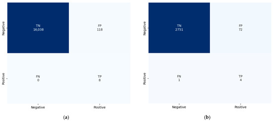
Figure 3.
(a) Confusion matrix of a SVM after 3σ preprocessing of the 1st dataset. (b) Confusion matrix of a SVM after 3σ preprocessing of the 2nd dataset.
The comparison of machine learning model performance revealed noticeable variations in both accuracy and GM depending on the applied preprocessing methods. Among the models, the SVM consistently demonstrated relatively stable and robust performance across different outlier detection methods, including MAD, IQR, and SDCL, as well as under various scaling techniques and process condition changes. When evaluating the preprocessing effects across datasets and processes, the KNN model exhibited instability under certain conditions. For instance, a substantial decrease in GM was observed with the MAD-based detection, while performance improved under the 3σ-based detection. This indicates sensitivity to the chosen outlier thresholding method. These results suggest that the selection of outlier detection criteria (e.g., MAD, IQR, SDCL) and data preprocessing strategies (e.g., scaling) significantly affects classification performance. Furthermore, the impact of these factors varies depending on the model architecture.
6. Conclusions
Latent defects in high-precision electronic devices and semiconductors are exposed to performance degradation risks when subjected to environmental factors and electrical stress during real-world operation. To ensure the reliability of products prior to shipment, it is therefore essential to conduct high-intensity stress testing that closely mimics actual operating conditions an approach that has a direct impact on manufacturing yield. In response to these challenges, this study proposes a post process prediction method utilizing various machine learning models to detect latent defects prior to screening tests. Data were obtained from devices that passed standard testing at SCK and subsequently subjected to preprocessing and SDCL. The results indicate that, under ±3σ preprocessing, all models except the DT achieved over 90% accuracy and GM. Notably, the SVM model consistently maintained the most stable performance across all preprocessing conditions. The proposed SDCL method labels devices based on the number of statistical outliers in their test features. Specifically, for each feature, device-level test results that fall outside the ±2σ or ±3σ range assuming a normal distribution are counted as anomalies. The total count of such feature-level anomalies is then used to label devices as either normal or potentially defective, based on threshold values again set at ±2σ or ±3σ. Furthermore, to accommodate the possibility of non-normal data distributions, additional labeling was performed using anomaly counts derived from the MAD and IQR methods.
Experimental results using both the primary and secondary datasets demonstrated that the proposed SDCL method achieved more generalized and stable performance compared to MAD and IQR approaches. Unlike methods that are sensitive to specific dataset characteristics, SDCL exhibited stronger potential for broad applicability. These findings indicate that SDCL effectively captures the characteristics of the data and offers a promising approach for the early prediction of performance degradation in initially normal products.
7. Discussion
This study proposed the SDCL method, a machine learning-based approach for the detection of latent defects. Experiments were conducted using two datasets provided by SCK, designed to verify whether the model could maintain consistent performance even when the product test parameters were altered. Experimental results showed that the SVM model exhibited the most stable performance regardless of preprocessing techniques or changes in dataset composition. Notably, data preprocessing based on the ±3σ threshold led to overall improvements in model accuracy. Furthermore, increasing the strictness of the outlier detection threshold resulted in better model performance across all models. These findings suggest that even among products that have passed initial screening, certain devices suspected of latent defects may form distinguishable clusters. The proposed SDCL-based machine learning methodology offers practical utility for anomaly detection and quality management automation. However, successful deployment in real-world manufacturing environments requires sufficient prior efforts in data collection, preprocessing, and the configuration of context specific threshold parameters. In the early stages of implementation, additional investment is needed for infrastructure capable of collecting and analyzing process data, as well as time and expert resources for model training.
This study employed traditional machine learning models in combination with the SDCL technique, leveraging various algorithms to account for the high dimensionality of the data and the potential linear and nonlinear relationships with the target variable. Nonetheless, several limitations remain. First, the study is based on a specific experimental dataset, and its application in actual manufacturing processes necessitates the careful calibration of boundary conditions that reflect process characteristics. Threshold values such as those derived from MAD, IQR, ±2σ, and ±3σ must be appropriately tuned according to process variability and required quality levels. For instance, in industries demanding high reliability such as automotive semiconductors stricter thresholds (e.g., ±2σ or ±3σ) are typically required, whereas in less precision sensitive domains, looser bounds (e.g., ±3σ or ±4σ) may be more appropriate. Second, the presence of high dimensional input features and process variability may hinder model generalization, thereby limiting the transferability of trained models across different production lines. To address this, future work will focus on incorporating ensemble learning methods and advanced hyperparameter optimization techniques to enhance model stability and performance. Moreover, the extension of this approach to deep learning models is recommended. In manufacturing scenarios where defect data are limited and imbalanced, the application of deep learning architectures such as Convolutional Neural Networks (CNN) or autoencoders is expected to enable the extraction of high-level features, suppression of noise, and more precise identification of latent defect patterns. Furthermore, for real time deployment, especially at the chip level, future studies must investigate methods for handling large scale data streams, enabling timely and efficient anomaly detection within high throughput production environments.
Author Contributions
Conceptualization, C.-s.N.; methodology, C.-s.N.; software, Y.-s.K., W.-c.S., H.-j.P. and H.-y.Y.; validation, C.-s.N., Y.-s.K. and W.-c.S.; formal analysis, Y.-s.K., W.-c.S.; investigation, W.-c.S.; resources, C.-s.N.; data curation, Y.-s.K., W.-c.S., H.-j.P. and H.-y.Y.; writing—original draft preparation, Y.-s.K. and W.-c.S.; writing—review and editing, Y.-s.K., W.-c.S., H.-j.P., H.-y.Y. and C.-s.N.; visualization, Y.-s.K. and W.-c.S.; supervision, C.-s.N.; project administration, C.-s.N.; funding acquisition, C.-s.N. All authors have read and agreed to the published version of the manuscript.
Funding
This work was partly supported by the Institute of Information & Communications Technology Planning & Evaluation (IITP)-Innovative Human Resource Development for Local Intellectualization program grant funded by the Korea government (MSIT) (IITP-2025-RS-2023-00259678, 50%) and by INHA UNIVERSITY Research Grant (70477-1, 50%).
Data Availability Statement
The data that support the findings of this study are not publicly available because of a confidentiality agreement with SCK. Access to the data is restricted in accordance with the terms of this agreement to protect proprietary information.
Acknowledgments
This work was supported by data provided by STATS ChipPAC Korea (SCK). We are grateful to SCK for their valuable contribution to this research.
Conflicts of Interest
The authors declare no conflict of interest.
References
- Nguyen, M.H.; Kwak, S. Enhance Reliability of Semiconductor Devices in Power Converters. Electronics 2020, 9, 2068. [Google Scholar] [CrossRef]
- Liao, H.T. Reliability prediction and testing plan based on an accelerated degradation testing model. Int. J. Mater. Prod. Technol. Technol. 2004, 21, 402–422. [Google Scholar] [CrossRef]
- Julitz, T.M.; Schlüter, N.; Löwer, M. Scenario-Based Failure Analysis of Product Systems and their Environment. arXiv 2023, arXiv:2306.15694. [Google Scholar] [CrossRef]
- Kim, J.; Joe, I. Chip-Level Defect Analysis with Virtual Bad Wafers Based on Huge Big Data Handling for Semiconductor Production. Electronics 2024, 13, 2205. [Google Scholar] [CrossRef]
- Price, D.W.; Sutherland, D.G.; Rathert, J. Process Watch: The (Automotive) Problem with Semiconductors. Solid State Technol. 2018, 15, 1–5. [Google Scholar]
- Qiao, X.; Jauw, V.L.; Seong, L.C.; Banda, T. Advances and limitations in machine learning approaches applied to remaining useful life predictions: A critical review. Int. J. Adv. Manuf. Technol. 2024, 133, 4059–4076. [Google Scholar] [CrossRef]
- Ooi, M.P.-L.; Kassim, Z.A.; Demidenko, S. Shortening Burn-in Test: Application of Weibull Statistical Analysis & HVST. In Proceedings of the 2005 IEEE Instrumentation and Measurement Technology Conference, Ottawa, ON, Canada, 16–19 May 2005; Volume 1, pp. 1–6. [Google Scholar] [CrossRef]
- Suhir, E. To Burn-In, or Not to Burn-In: That’s the Question. Aerospace 2019, 6, 29. [Google Scholar] [CrossRef]
- Wang, M. A Review of Reliability in Gate-All-Around Nanosheet Devices. Micromachines 2024, 15, 269. [Google Scholar] [CrossRef]
- Lenhard, P.; Kovalenko, A.; Lenhard, R. Die Level Predictive Modeling to Reduce Latent Reliability Defect Escapes. Microelectron. Reliab. 2023, 148, 115139. [Google Scholar] [CrossRef]
- Moreno-Lizaranzu, M.J.; Cuesta, F. Improving Electronic Sensor Reliability by Robust Outlier Screening. Sensors 2013, 13, 13521–13542. [Google Scholar] [CrossRef] [PubMed]
- Pihlaja, D. Real Time Dynamic Application of Part Average Testing (PAT) at Final Test. In Proceedings of the CS MANTECH Conference, New Orleans, LA, USA, 13–16 May 2013; pp. 165–167. [Google Scholar]
- Wang, C.-C.; Yang, Y.-Y. A Machine Learning Approach for Improving Wafer Acceptance Testing Based on an Analysis of Station and Equipment Combinations. Mathematics 2023, 11, 1569. [Google Scholar] [CrossRef]
- Hu, H.; Patel, S.; Hsiao, H.; Tretz, F.; Volk, T.; Arslan, M.; Nix, R.; Jindal, S.; Archambeault, B. Advanced Outlier Detection Using Unsupervised Learning for Screening Potential Customer Returns. In Proceedings of the 2020 IEEE International Test Conference, Washington, DC, USA, 2–5 November 2020; pp. 1–10. [Google Scholar] [CrossRef]
- van Selst, M.; Jolicoeur, P. A Solution to the Effect of Sample Size on Outlier Elimination. Q. J. Exp. Psychol. Sect. 1994, 50, 386–393. [Google Scholar] [CrossRef]
- Yang, J.; Rahardja, S.; Fränti, P. Outlier Detection: How to Threshold Outlier Scores? In Proceedings of the International Conference on Artificial Intelligence, Information Processing and Cloud Computing, New York, NY, USA, 19–21 December 2019; pp. 1–6. [Google Scholar]
- Wan, X.; Wang, W.; Liu, J.; Tong, T. Estimating the Sample Mean and Standard Deviation from the Sample Size, Median, Range and/or Interquartile Range. BMC Med. Res. Methodol. 2014, 14, 135. [Google Scholar] [CrossRef]
- Dhwani, D.; Varma, T. A Review of Various Statistical Methods for Outlier Detection. Int. J. Comput. Sci. Eng. Technol. 2014, 5, 137–140. [Google Scholar]
- Wickham, H.; Stryjewski, L. 40 Years of Boxplots. Am. Stat. 2011, 65, 1–6. [Google Scholar]
- Jones, P.R. A Note on Detecting Statistical Outliers in Psychophysical Data. Atten. Percept. Psychophys. 2019, 81, 1189–1196. [Google Scholar] [CrossRef] [PubMed]
- Atif, M.; Farooq, M.; Shafiq, M.; Alballa, T.; Alhabeeb, S.A.; Khalifa, H.A.-E.-W. Uncovering the Impact of Outliers on Clusters’ Evolution in Temporal Data-Sets: An Empirical Analysis. Sci. Rep. 2024, 14, 30674. [Google Scholar] [CrossRef]
- França, C.M.; Couto, R.S.; Velloso, P.B. Missing Data Imputation in Internet of Things Gateways. Information 2021, 12, 425. [Google Scholar] [CrossRef]
- Emmanuel, T.; Tlamelo, M.; Phaneendra, B.; Das, D.; Epule, E. A Survey on Missing Data in Machine Learning. J. Big Data 2021, 8, 140. [Google Scholar] [CrossRef]
- Kang, H. The Prevention and Handling of the Missing Data. Korean J. Anesth. 2013, 64, 402–406. [Google Scholar] [CrossRef]
- Chandrashekar, G.; Sahin, F. A Survey on Feature Selection Methods. Comput. Electr. Eng. 2014, 40, 16–28. [Google Scholar] [CrossRef]
- Jizat, J.A.M.; Ahmad, N.; Alwi, N.H.; Nor, M.I.; Salleh, N.M.; Kamal, M.M. Evaluation of the Machine Learning Classifier in Wafer Defects Classification. ICT Express 2021, 7, 535–539. [Google Scholar] [CrossRef]
- Hu, J.; Zhou, Z.; Chen, J.; Wang, Z.; Lin, S.; Li, Y. A Novel Quality Prediction Method Based on Feature Selection Considering High Dimensional Product Quality Data. J. Ind. Manag. Optim. 2022, 18, 2715–2735. [Google Scholar] [CrossRef]
- Taha, K. Observational and Experimental Insights into Machine Learning-Based Defect Classification in Wafers. J. Intell. Manuf. 2025, 020502. [Google Scholar] [CrossRef]
- Lee, Y.; Roh, Y. An Expandable Yield Prediction Framework Using Explainable Artificial Intelligence for Semiconductor Manufacturing. Appl. Sci. 2023, 13, 2660. [Google Scholar] [CrossRef]
- Barandela, R.; Valdovinos, R.M.; Sánchez, J.S.; Ferri, F.J. The Imbalanced Training Sample Problem: Under or Over Sampling? In Proceedings of the Structural, Syntactic, and Statistical Pattern Recognition, Lisbon, Portugal, 18–20 August 2004; Structural, Syntactic, and Statistical Pattern Recognition. Springer: Berlin/Heidelberg, Germany, 2004; Volume 3138, pp. 806–814. [Google Scholar]
- García, V.; Sánchez, J.S.; Mollineda, R.A. On the Effectiveness of Preprocessing Methods When Dealing with Different Levels of Class Imbalance. Knowl.-Based Syst. 2012, 25, 13–21. [Google Scholar] [CrossRef]
Disclaimer/Publisher’s Note: The statements, opinions and data contained in all publications are solely those of the individual author(s) and contributor(s) and not of MDPI and/or the editor(s). MDPI and/or the editor(s) disclaim responsibility for any injury to people or property resulting from any ideas, methods, instructions or products referred to in the content. |
© 2025 by the authors. Licensee MDPI, Basel, Switzerland. This article is an open access article distributed under the terms and conditions of the Creative Commons Attribution (CC BY) license (https://creativecommons.org/licenses/by/4.0/).