Lifetime Prediction of GaN Power Devices Based on COMSOL Simulations and Long Short-Term Memory (LSTM) Networks

Abstract

Gallium nitride (GaN) power devices have attracted extensive attention due to their superior performance in high-frequency and high-power applications. However, the reliability and lifetime prediction of these devices under various operating conditions remain critical challenges. In this study, a hybrid approach combining finite element simulation and deep learning is proposed to predict the lifetime of GaN power devices. COMSOL Multiphysics (V6.3) is employed to simulate the thermal and mechanical stress behavior of GaN devices under different power and frequency conditions, while capturing key degradation indicators such as temperature cycles and stress concentrations. The variation in temperature over time can reflect the degradation of the device and also reveal the fatigue damage caused by the long-term accumulation of thermal stress on the chip. LSTM performs exceptionally well in extracting features from time series data, effectively capturing the long-term and short-term dependencies within the time series. By using simulation data to establish a connection between the chip temperature and its service life, the temperature data and the lifespan data are combined into a dataset, and the LSTM neural network is used to explore the impact of temperature changes over time on the lifespan. The method mentioned in this paper can make preliminary predictions of the results when sufficient experimental data cannot be obtained in a short period of time. The prediction results have a certain degree of reliability.

1. Introduction

Gallium nitride (GaN) power devices have emerged as a transformative technology in the field of power electronics due to their exceptional material properties, including wide bandgap, high electron mobility, and high breakdown voltage [1,2,3,4]. These advantages enable GaN-based devices to operate at higher frequencies, voltages, and power densities compared to traditional silicon-based counterparts. As a result, GaN devices have found increasing applications in high-frequency switching power supplies, electric vehicles, RF amplifiers, and aerospace systems. However, the harsh operational environments and high thermal loads associated with these applications raise significant concerns regarding the long-term reliability and operational lifetime of GaN power devices.

Device lifetime is a critical metric in power electronics, directly impacting system reliability, maintenance cycles, and safety. Premature failure of power devices can lead to catastrophic system malfunctions, especially in mission-critical applications. Therefore, accurately predicting the lifetime of GaN power devices under varying operational conditions is essential for robust design and reliable deployment. Lifetime prediction typically involves understanding the degradation mechanisms driven by thermal, electrical, and mechanical stresses accumulated over time. These mechanisms include thermal cycling fatigue [5], electromigration [6], and stress-induced delamination [7], all of which are influenced by device structure, material properties, and loading profiles such as power levels and switching frequency. Conventional approaches to lifetime prediction often rely on empirical models derived from accelerated aging tests, such as Arrhenius-type models [8], Coffin–Manson relationships [5], and rainflow counting methods [9]. While these models provide useful approximations, they are limited by several inherent shortcomings. First of all, they require a large amount of experimental data, and obtaining this data requires a lot of equipment and a considerable amount of time, which cannot be accomplished within a short period of time. However, the prediction of the lifespan of gallium nitride chips is extremely dependent on relevant data with temporal characteristics. Second, they often assume simplified and static loading conditions, failing to capture the dynamic behaviors of devices in real-world operations. Third, many methods require collecting data information from multiple dimensions, and the data collection process is quite challenging. Among the common failure modes, a large number of failures can be reflected by the temperature changes over time, such as lead bonding failure and thermal breakdown. The change in temperature can be regarded as a relatively common factor reflecting the working state of the chip.

To address these limitations, this study proposes a hybrid method that combines multiphysics finite element simulation with a data-driven deep learning approach [10,11,12] to predict the lifetime of GaN power devices. Specifically, COMSOL Multiphysics is utilized to simulate the thermal and mechanical stress distribution in GaN devices [13,14,15] under various power and frequency settings. These simulations provide detailed insight into the spatiotemporal evolution of temperature fields, stress concentrations, and fatigue-inducing cycles, which are difficult to capture experimentally. We combined temperature and fatigue life to create a dataset and used the temperature data in conjunction with physical formulas to characterize the degradation process of the chip. To extract patterns from this time-series data and forecast future degradation trends, a Long Short-Term Memory (LSTM) neural network is employed [16,17,18,19,20,21]. LSTM, a variant of recurrent neural networks (RNNs), is particularly well-suited for modeling temporal sequences and capturing long-term dependencies. By using a long short-term memory model trained on simulated data, this model is able to learn the complex relationship between temperature changes over time and the lifespan of the chip, thereby being capable of accurately predicting the lifespan for situations that have not been encountered before. This approach significantly reduces the reliance on large-scale physical aging experiments and enhances the adaptability of lifetime modeling to diverse device configurations and operating environments.

Unlike traditional feedforward neural networks, the Long Short-Term Memory (LSTM) architecture incorporates memory units and gating mechanisms, which enable it to retain long-term temporal dependencies [22,23] and alleviate the problem of gradient vanishing, which is crucial for capturing the time-varying temperature characteristics in power devices. This capability allows LSTM to learn the complex nonlinear relationships between historical operating conditions (the amplitude and speed of temperature changes) and the final failure behavior of the devices. Most predictions of service life are based on the characteristic that certain physical quantities of the object to be predicted change over time. Then, the trend in these characteristics over time is analyzed to establish a corresponding relationship with the final service life. LSTM can effectively extract these time-related features. The temperature of GaN devices is affected by various factors such as packaging and operating conditions. The final temperature change is manifested as a time-varying sequence. LSTM can extract many time-related features from this sequence, and by linking these features with the corresponding service life, the service life prediction of GaN chips can be achieved. LSTM, due to its ability to effectively extract time-related features, has been widely applied in the prediction of the lifespan of mechanical or electronic equipment [24]. Despite these advantages, applying LSTM to life prediction still involves several technical considerations. These include careful sequence design to ensure temporal coherence (the sampling time standard for all the tested chips is the same), appropriate normalization of input variables to maintain learning stability, and effective training strategies to prevent overfitting [25,26], particularly when the dataset is limited or simulated. Moreover, hyperparameter tuning (e.g., number of layers, hidden units, and learning rate) and evaluation using appropriate loss functions are critical to optimizing prediction accuracy. Attention must also be given to how well the model generalizes across unseen operating conditions, which is essential for robust real-world deployment.

In this paper, a comprehensive finite element modeling framework was developed using COMSOL to simulate the thermal–mechanical response of gallium nitride power chips under various operating conditions. A structured approach was adopted to convert the simulation results into data related to the attenuation situation. At the same time, a dataset related to the time series was constructed based on the simulation results. A prediction model based on deep learning and using Long Short-Term Memory (LSTM) was designed and trained, aiming to predict the service life of equipment. The results predicted by this model demonstrate a certain degree of reliability. The proposed methodology offers a scalable and efficient alternative to traditional lifetime prediction techniques, paving the way for intelligent reliability analysis in next-generation power electronics. The device selected for this study is the GaN HEMT MMIC PA. It is mainly used to amplify the weak radio frequency signal input to a higher power level and is also used to drive antennas or subsequent circuits. Overall, this work bridges the gap between physics-based simulation and data-driven prediction, providing a novel pathway toward more accurate and practical lifetime assessment for GaN power devices.

2. Simulation and Analysis

In this study, we investigated the typical degradation mechanisms of GaN power devices and proposed a novel lifetime prediction method based on the combination of finite element simulation and deep learning. Unlike traditional approaches that rely heavily on empirical models or statistical extrapolation from aging experiments, our method integrates COMSOL-based multiphysics simulations with a Long Short-Term Memory (LSTM) neural network to enhance prediction accuracy and generalizability under diverse operating conditions. To generate realistic degradation data, we employed COMSOL Multiphysics to simulate the thermal and mechanical stress distribution within GaN devices under different power loads and switching frequencies. COMSOL was selected over other tools such as ANSYS (2023 R1) Icepak due to its superior capabilities in coupling multiple physical domains—particularly thermal–mechanical interactions that are essential for capturing the fatigue-inducing mechanisms in GaN-based structures. Through these simulations, we obtained time-resolved stress and temperature fields, which reflect the evolution of critical failure precursors, such as thermal fatigue, delamination, and stress concentration near junction interfaces. In this study, the simulation modeling is not aimed at the specific modeling of transistors or semiconductors, but rather it is based on the thermodynamic modeling of chip power dissipation and the mechanical modeling of thermal stress caused by thermal expansion.

The detailed data of the chips used in this experiment are shown in

Table 1. The operating condition parameters of the chip.

Parameter	Value
DC terminal voltage $VDS$ (V)	36
Input signal power $\mathrm{P}\mathrm{i}\mathrm{n}$ (dBm)	44
Input signal pulse width (ns)	200
frequency $f$ (GHz)	9.0
Conduction resistance resistor (mΩ)	150
Power-added efficiency PAE (%)	38
Power Gain (dB)	9.0

,

Table 2. Internal structural dimensions of GaN FET.

Modular Structure	Length (mm)	Width (mm)	Height (mm)	Materials
Chip	1.5	1.3	0.05	GaN
Substrate	1.5	1.3	0.15	SiC
Chip soldering layer	1.52	1.32	0.3	Sn3.5Ag
Top copper layer	16.2	6.4	0.8	Cu
Ceramic layer	12.4	4.6	0.5	Al2O3
The under-soldering layer	12.4	4.6	0.5	Sn3.5Ag
Substrate	18.1	8.7	2.04	CPC

,

Table 3. Material characteristics of GaN FET.

Materials	Density (g/cm3)	Coefficient of Thermal Expansion (/10−6·K−1)	Thermal Conductivity (W/(m·K))	Young’s Modulus (GPa)	Poisson’s Ratio
GaN	6.10	5.59	130	275	0.215
W80Cu	15.65	8.30	200	276	0.310
SiC	3.20	5.00	270	354	0.190
Sn3.5Ag	7.30	21	54	47.2	0.4
CPC	9.20	9.50	260	120	0.320
Al2O3	3.60	6.50	30	270	0.222

and

Table 4. Finite element simulation load setting.

Simulation Load	Numerical Setting
Environmental temperature (°C)	20
Heat flux(W/mm2)	12.3
Thermal radiation	1
Thermal convection(W/mm2·°C)	5

. The content in Table 1 represents the working conditions parameters of the chips, the content in Table 2 shows the internal structural dimensions of the GaN FET, and the content in Table 3 presents the material characteristics of the GaN FET. Finite element simulation load setting in Table 4.

Unlike passive components such as capacitors, in which failure may manifest through parameter drift or electrolyte depletion, GaN device failure is more closely associated with accumulated thermal stress and material degradation caused by repetitive switching and self-heating cycles. Therefore, the simulated output is processed into a time series dataset related to temperature, where each sequence represents the evolution of the chip’s temperature under a specific operating scenario. These datasets were used to train multiple machine learning models for lifetime prediction. In this work, we primarily focus on the LSTM model due to its capability to learn long-range temporal dependencies in time-series data, which is essential for tracking gradual degradation patterns. While other methods like XGBoost, KNN, or feedforward neural networks (e.g., BP networks) may capture static relationships, they often struggle with the temporal dynamics inherent in device aging processes. LSTM, with its memory cells and gating mechanisms, offers a more suitable architecture for predicting remaining useful life (RUL) based on sequential stress responses.

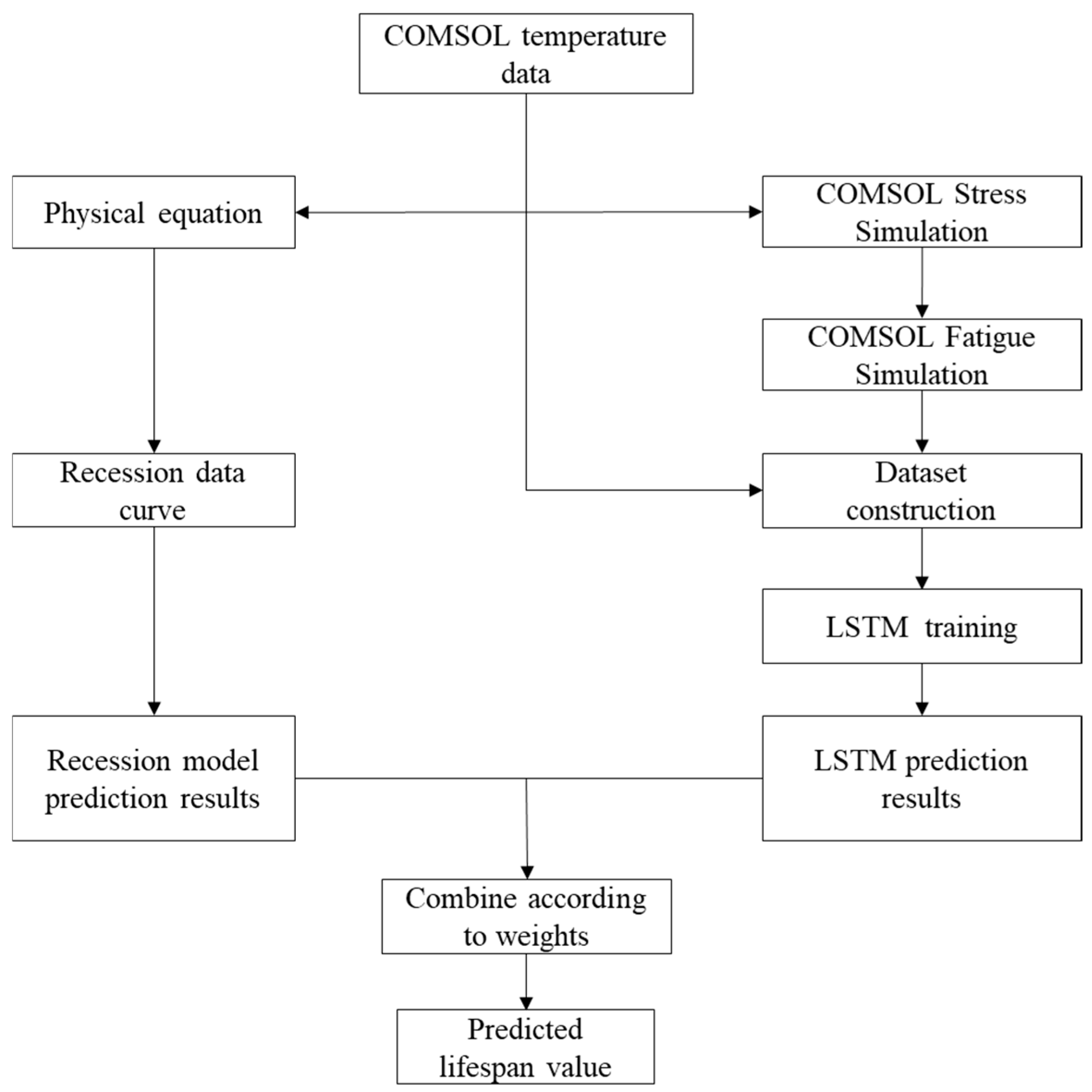
It is important to note that when applying LSTM to lifetime prediction tasks, several technical considerations must be addressed. These include the appropriate segmentation and normalization of input sequences, careful selection of model depth and hidden units, and rigorous validation using cross-validation techniques to prevent overfitting, especially when the dataset is simulation-based and limited in diversity. Furthermore, model generalizability across various loading conditions and device geometries must be ensured to enable broader application in real-world scenarios. The flowchart for predicting the lifespan of the device using the hybrid model is shown in Figure 1. 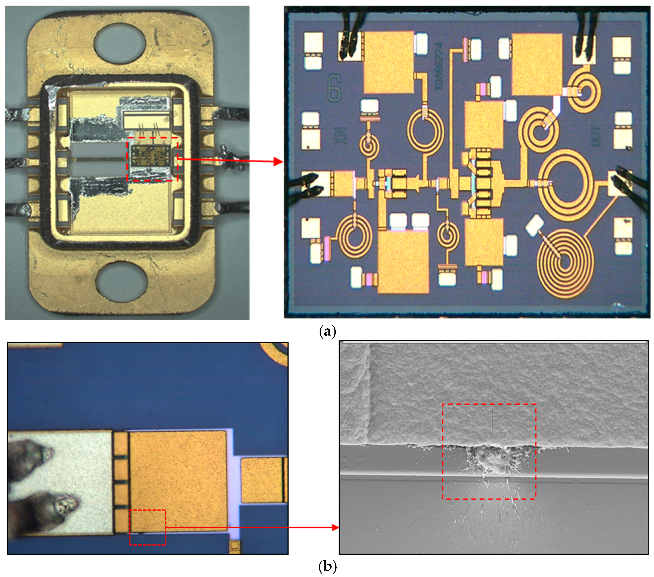Figure 2a summarizes the primary degradation modes observed in GaN power devices under repeated thermal-electrical cycling, including thermal fatigue-induced cracking, increased junction resistance, and material delamination. In our experimental investigation, a mechanical decapsulation technique was employed to open the device packages, aiming to identify structural anomalies or internal defects potentially associated with observed failure modes and to accurately locate the failure sites. After decapsulation, optical microscopy was used to examine the internal structure of the samples in detail. The result is shown in Figure 2b. The post-decapsulation inspection revealed several significant failure-related features. Because the voltage borne by the capacitor medium exceeded the designed withstand voltage value, a concentrated local electric field was formed, resulting in dielectric breakdown. Specifically, the gate bonding wire was found to be melted and broken, indicating a possible overcurrent or localized overheating event. Additionally, thermal discoloration marks were observed at the die-attach interface between the chip and the substrate, suggesting excessive heat accumulation during device operation. Sooting and deposition of splattered molten bonding wire material were also noted on the inner surface of the metal lid, which further supports the occurrence of high-temperature events leading to bond wire failure. No other anomalies were observed in the remaining regions of the device. These findings point to a thermal-electrical failure mechanism, likely initiated by localized Joule heating or thermal runaway at the gate terminal. The observed internal morphology and failure traces after decapsulation provide visual evidence to support the failure analysis.

The fabrication process of GaN devices can be divided into four core steps: substrate selection, epitaxial growth, device structure preparation, and passivation and packaging. Among them, the substrate and epitaxy are the key factors determining the performance and cost of the device. Although the GaN single crystal substrate is perfectly matched with the GaN crystal lattice, its preparation is difficult, and the cost is extremely high (5–10 times that of a SiC substrate). Currently, the mainstream method is to use hetero substrates and achieve high-quality GaN epitaxial layer growth through “lattice mismatch compensation”. Epitaxial growth is the process of growing a single layer or multiple layers of GaN-based materials (such as GaN, AlGaN, InGaN) on the substrate. It directly determines the crystal quality (defect density) of the material and the reliability of the device. MOCVD (Metal–Organic Chemical Vapor Deposition) is the current mainstream production technology. The device structure preparation step forms the core functional area of the device through semiconductor micro-processing technology. The key steps include: lithography and etching, ohmic contact preparation, Schottky contact preparation, and ion implantation. The surface states of GaN devices are easily affected by the environment, and in high-power scenarios, heat dissipation is concentrated, which requires a solution through passivation and packaging.

A variety of factors can lead to excessive leakage current and eventual failure in electrolytic capacitors. These include inadequate manufacturing processes, poor oxide film formation, outdated slicing techniques, physical damage or contamination of the oxide layer, suboptimal electrolyte formulation, low-purity raw materials, and instability in the chemical or electrochemical properties of the electrolyte over time. In particular, high chloride ion contamination can accelerate oxide film degradation, leading to localized perforation and increased leakage current. Impurities such as copper and silicon hinder the proper formation of crystalline aluminum oxide, further exacerbating leakage issues. In the manufacturing process of GaN devices, chlorine-based gases (such as Cl₂, BCl₃, and HCl) are commonly used for etching or cleaning. The residual chlorine ions are prone to causing contamination. The chloride ions (Cl⁻) can easily lead to metal corrosion, electrode failure, increased leakage current, and reliability risks. Copper impurities usually come from electrode materials, while silicon usually originates from the glass fiber support material. Even if other different oxides are used, impurity contamination still has an impact, although the manifestation may be different. Overall, metallic impurities significantly contribute to increased leakage current and reduced capacitor lifespan. To predict component lifespan, simulations were conducted using COMSOL and compared with experimental data. The simulated results deviated by no more than 5% from actual measurements.

3. Result

• COMSOL simulation process

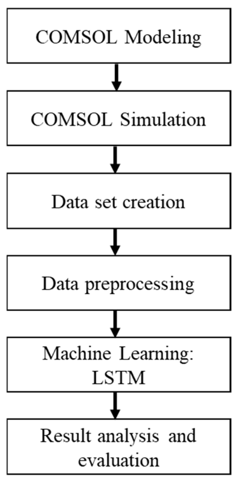
The simulation process of GaN power devices is conducted on the COMSOL Multiphysics platform, employing a multiphysics coupling modeling approach to systematically evaluate the thermal and mechanical response characteristics of the devices under complex operating conditions. The entire simulation workflow is shown in Figure 3.

Initially, simulation preparation is conducted to define the target scenario and physical processes. Subsequently, model parameters are determined in COMSOL, where thermal conductivity, thermal expansion coefficient, and other material properties of GaN are input, and the geometric model of the device structure is constructed. Following this, the necessary boundary conditions and initial parameters, such as thermal dissipation paths and ambient temperature, are configured. Upon completion of the model setup, the multiphysics coupling analysis phase is initiated. First, the actual experimental data of electrothermal heat generation is imported into COMSOL as a heat source. Then, through thermodynamic simulation, the heat distribution of the packaged device under natural cooling conditions during operation is obtained and saved. At the same time, the coupled simulation of thermal–mechanical is continued to simulate the thermal stress distribution caused by the temperature gradient and evaluate the potential impact of stress fatigue on the packaging structure.

Upon completion of the coupling modeling, the simulation model is executed to yield results such as temperature fields and stress fields. The simulation data is processed using COMSOL’s visualization tools to further analyze the effects of different power densities and packaging structure parameters on thermal management efficacy, and to explore the correlation between temperature rise, stress concentration, and device reliability degradation. This simulation workflow fully leverages COMSOL’s strengths in multiphysics coupling computation and parameter visualization, providing robust support for the structural optimization and reliability design of GaN power devices.

In the COMSOL simulation, we simulate the working mode of the chip by conducting periodic thermal power cycling tests. In actual testing, we monitor the drift of the change in power, combine infrared thermal imaging to locate hotspots of the metal capacitor, and analyze failures such as solder layer peeling or gate metal electrical migration. The test conditions need to control ΔT, the heating and cooling rate (>100 °C/s), and the duty cycle (10–90%) to accelerate the fatigue accumulation. Power cycling test: directly correlates with the high-frequency switching condition to verify the deviation between the thermal simulation based on the dissipated power inputs model in the simulation and the experimental data. Use the actual power cycling test results as the basis for the COMSOL simulation to prove the validity of the COMSOL simulation.

The thermal distribution data obtained from the COMSOL simulation is input into the Weibull–Arrhenius equation to obtain the degradation curve of the equipment. When the equipment degrades to 80%, it is considered to have failed, and a set of lifetime data is obtained. This lifetime value will be combined with the predicted lifetime obtained by LSTM at a certain weight as the final predicted lifetime value.

During the multi-physics simulation process, in order to more accurately reflect the thermal response behavior of GaN power chips under actual working conditions, we introduced a modeling method of dynamic power waveform input in COMSOL Multiphysics. Specifically, based on the geometric structure and thermal simulation based on dissipated power inputs model that were previously constructed, by applying time-varying power signals to the heat source term, we simulated the operating state of the chip under periodic on-off or variable power load conditions.

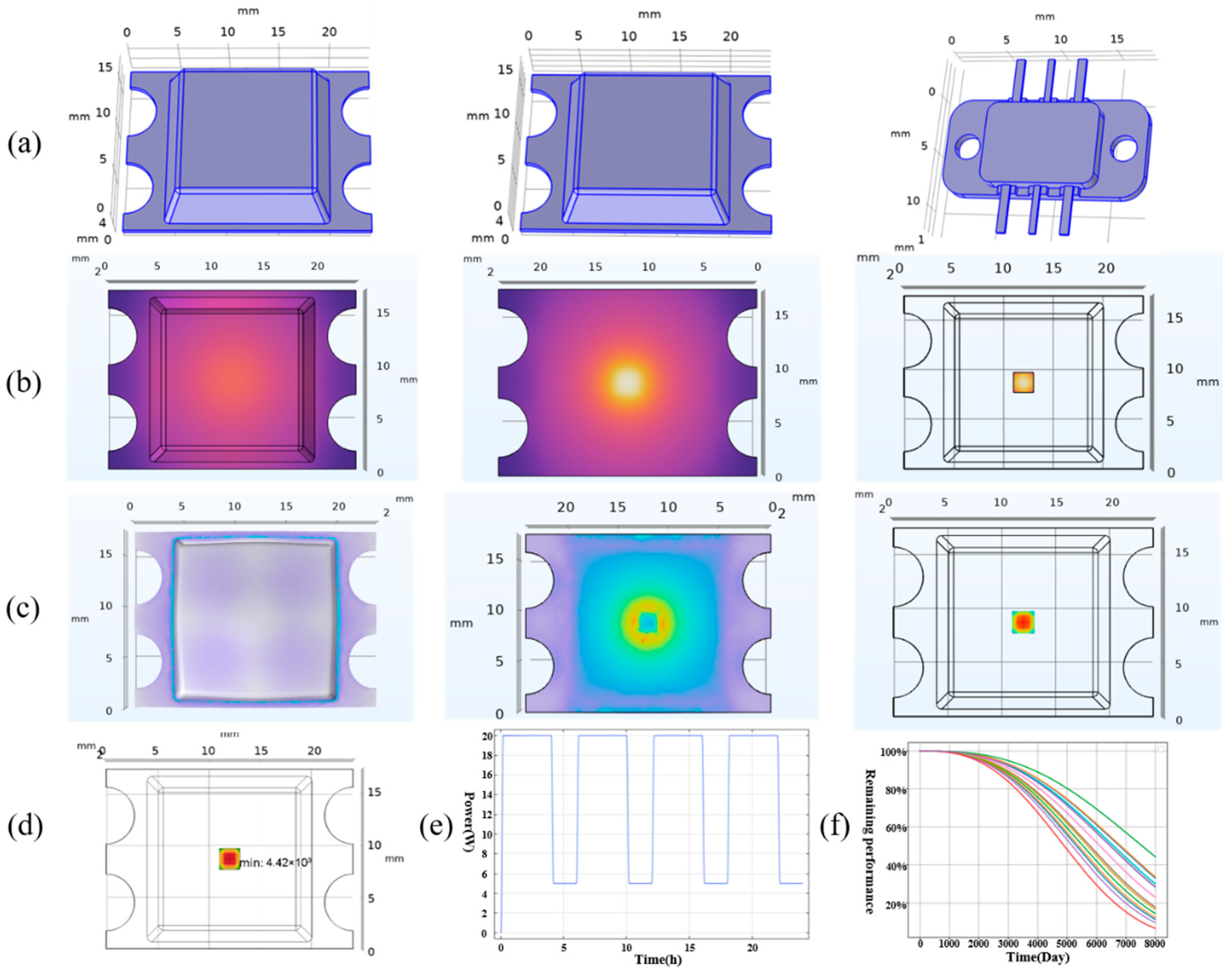
The packaging modeling of different devices is shown in Figure 4a. The heat source is positioned in the middle part of the chip package, close to the bottom layer. The heat flux is set as convective heat flux with air as the medium. The convective heat transfer coefficient is set to 10 (W/(m²·K)), and the external environment temperature is set to 293.15 [K]. We characterize the heating condition of the heat source by using square wave heat power. Different square wave powers and duty ratios represent the power consumption under different working modes. The power waveform is shown in Figure 4e. Here, the power amplitude represents the maximum power consumption level of the chip during conduction, while the duty cycle is used to simulate the conduction ratio of the chip within a unit time. By adjusting these two parameters, the thermal behavior of the device under various operating conditions such as low-frequency high load and high-frequency low load can be flexibly simulated.

After the model is adjusted, it is solved in COMSOL through the “time-dependent” module. The system can automatically respond to the changes in the power waveform within the time domain, and calculate the corresponding transient temperature distribution and thermal stress evolution. The temperature data is then incorporated into the physical model Weibull–Arrhenius (The specific formula of this model will be elaborated in the next part of the article.) to obtain the attenuation of the device’s output power over time as shown in Figure 4f (multiple different samples). A total of 300 simulation attenuation data points were collected for this project. This demonstrates the evolution process of the chip’s thermal field under different input power conditions. This method not only improves the authenticity and dynamic response capability of thermal simulation, but also provides an important means for evaluating the thermal management effect and reliability of the chip in typical application scenarios such as pulse load and intermittent operation.

During the COMSOL simulation process, the acquisition of temperature distribution is one of the key steps in evaluating the thermal performance of power electronic devices. For high-power density electronic devices such as GaN, the spatial distribution of the temperature field not only directly affects the electrical performance and reliability of the device, but also relates to the stability and safety of its long-term operation. Especially under different packaging structures, the differences in heat conduction paths, thermal resistance distribution, and material thermal conductivity will lead to significant temperature gradients within the device, thereby affecting the overall heat dissipation efficiency. Therefore, accurately simulating and analyzing the temperature distribution has the following important significances: (1) It can identify the hotspots in the chip, providing a basis for material selection and structure optimization; (2) It helps evaluate the thermal diffusion capability of the packaging structure and determine whether it is suitable for high-power applications; (3) It provides a foundation for subsequent thermal–mechanical coupling analysis, predicting the thermal stress concentration and potential failure risks caused by temperature non-uniformity.

In this project, based on three typical packaging forms, we used the COMSOL thermal simulation based on the dissipated power inputs module to obtain the steady-state and transient temperature distribution inside the device under different operating conditions. As shown in Figure 4b, it presents the typical temperature field distribution characteristics of the chip under a specific power input, providing quantitative support for deeply understanding the impact of packaging design on thermal management performance. At the same time, this temperature data was exported to an Excel table for convenient future use.

In the multi-physics field simulation of power electronic devices, apart from the temperature distribution itself, the thermal stress distribution caused by the temperature gradient also has significant engineering significance. Due to the variety of materials inside the chip and the differences in thermal expansion coefficients, after the device is powered on and generates heat, the unevenness of the temperature distribution will cause complex thermal stress concentration at different material interfaces and structural edges. Over a long period, this accumulation may lead to material fatigue, crack initiation, and even failure of the packaging layer or solder joints. In this study, we utilized the thermal-structural coupling module of COMSOL to further solve the stress field inside the device based on the obtained temperature field distribution, and focused on analyzing the stress concentration areas at the chip surface and interfaces. By introducing mechanical parameters such as the material thermal expansion coefficient, Young’s modulus, and Poisson’s ratio, we simulated the deformation and contact state of each structural unit under the temperature rise condition.

The simulation results are shown in Figure 4c, which reveal the evolution law of thermal stress within the chip under different packaging forms and power conditions. The study indicates that the high-temperature hotspots often correspond to high-stress concentration areas, especially at the chip-substrate interface. By comparing the stress distributions of different structural models, it is helpful to identify potential reliability weak points, thereby enabling structural reinforcement or material selection optimization during the packaging design stage. Thermal stress simulation not only provides support for the thermal management of the device but is also an indispensable part of achieving high-reliability power device design.

After obtaining the distribution of the stress field, the data is used for the stress-life simulation in the COMSOL fatigue simulation. The module’s built-in S-N curve model is applied to calculate the device’s lifespan, as shown in Figure 4d.

2.

Recession Model and LSTM Construction

In the research, we adjusted the temperature data obtained from the COMSOL simulation based on the data from the accelerated decline test. Accelerated recession experimental data are shown in

Table 5. Accelerated recession experimental data.

Chip Type	Duration of Aging (h)	Serial Number	Tone-Up (dB)
NC912P1	0	1	15.1
		2	15.2
		3	15.1
P39		1	11
		2	11
		3	11
P34		1	16.56
		2	16.5
		3	16.5
NC912P1	148	1	14.28
		2	14.67
		3	14.48
P39		1	10.49
		2	10.32
		3	10.37
P34		1	15.37
		2	15.48
		3	15.48
NC912P1	314	1	14.17
		2	14.39
		3	14.22
P39		1	10.11
		2	10.04
		3	10.06
P34		1	15.12
		2	15.18
		3	15.14
NC912P1	426	1	14.02
		2	14.11
		3	14.05
P39		1	9.97
		2	9.88
		3	9.91
P34		1	14.87
		2	14.91
		3	14.87
NC912P1	1032	1	13.96
		2	13.99
		3	14.01
P39		1	9.86
		2	9.79
		3	8.82
P34		1	14.73
		2	14.79
		3	14.68

.

After obtaining the heat field data through COMSOL simulation, this project, based on the basic theory of the Weibull distribution model and in combination with the parameter attenuation characteristics of GaN power devices, studies the multi-field coupling by integrating the Weibull model and the Arrhenius model, and establishes the formula:

$$R(t,T)=\mathrm{e}\mathrm{x}\mathrm{p}\left(-{\left({\displaystyle \frac{t}{\tau (T)}}\right)}^{\alpha }\right)$$

(1)

$$\tau (T)={\tau }_0\cdot \mathrm{e}\mathrm{x}\mathrm{p}\left({\displaystyle \frac{E_a}{k_B{T}_{avg}}}\right)$$

(2)

Among them: $\alpha$ is 3, ${\tau }_0$ is the time factor with a value of 2 × 10⁻⁸, $E_a$ is the activation energy of the specific device, $k_B$ is the Boltzmann constant with a value of 8.617 × 10⁻⁵ eV/K. The graph plotted based on the established Weibull–Arrhenius formula is shown in Figure 4f. After substituting the COMSOL thermal simulation data, the attenuation curve of the equipment can be obtained. Combining the heat distribution data with the fatigue life to establish a dataset, it is used for machine learning (long short-term memory neural network) to conduct regression analysis on the simulation data, in order to improve the prediction accuracy under complex conditions.

As shown in Figure 5, in this project, in order to accurately predict the lifespan of GaN power devices, we have constructed a lifespan modeling process that integrates physical modeling and data-driven algorithms, as depicted in the figure. The entire process begins in the data preparation stage, where the thermal distribution data obtained from the COMSOL simulation is combined with the fatigue life data. These data are then used as the training dataset for the neural network. After completing the data collection, data cleaning is performed first to eliminate outliers and missing values, ensuring data quality.

During the modeling stage, this flowchart illustrates two key components: On one hand, the COMSOL simulation thermal distribution data is processed, and the fatigue life values are used as labels to obtain the dataset; on the other hand, the dataset is used for LSTM training to capture the temporal characteristics of the data and confirm that the model error is controlled within 10%. Finally, based on the trained model, it can be used to optimize the power density design of the device, improve the thermal management structure of the package, and provide theoretical support and data decision-making basis for the long-term reliability improvement of the device. This process fully integrates the COMSOL physical field simulation results with the data-driven prediction mechanism and constructs a complete lifespan modeling framework from simulation to intelligent prediction.

For the machine learning part, the Long Short-Term Memory neural network (LSTM) was selected as an improved variant of the Recurrent Neural Network (RNN). It demonstrates significant advantages in processing sequential data. The standard RNN has difficulty capturing long-distance temporal dependencies due to the “gradient vanishing/exploding” problem when dealing with long sequences. LSTM, through “gate units” (input gate, forget gate, output gate), controls the flow of information and allows the model to selectively retain or forget long-term information, thus effectively handling the dependencies in long sequences.

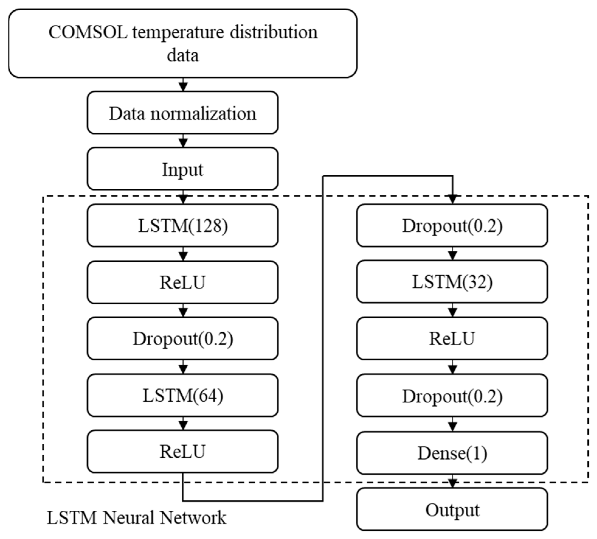
The data of each sample is stored in an Excel table. Each Excel file represents a sample, and each column in the Excel file represents a time step. The file name of the Excel file is used as the label for the sample’s lifespan. Due to the large amount of data information and large data values, to accelerate the learning rate of the neural network, the data of all samples is normalized using the maximum and minimum values, and all lifespan labels are also normalized using the maximum and minimum values. After processing, all data and lifespan labels will be proportionally scaled to 0–1, thereby compressing the data values and accelerating the learning efficiency. The neural network uses a three-layer LSTM, with a ReLU activation function layer and a Dropout layer after each layer.

ReLU (the Rectified Linear Unit) is one of the most commonly used activation functions in deep learning. Its core idea is to introduce nonlinear characteristics while alleviating the problem of gradient disappearance. Dropout is a widely used regularization technique in deep learning. Its core idea is to randomly “discard” (temporarily ignore) a portion of neurons during training to reduce the model’s dependence on specific features, enhance generalization ability, and alleviate overfitting problems. Finally, it outputs through the fully connected layer. The specific structure is shown in Figure 6.

Take 20% of the sample as the test set, 80% as the training set, and 20% as the validation set. The loss function is selected as MSE, which is a commonly used loss function in machine learning and statistics, used to measure the difference between the predicted values and the true values. Its core idea is to quantify the accuracy of the prediction by calculating the mean square error, and the smaller the value, the better the prediction effect. The optimizer is chosen as Adam, with the learning rate set to 0.0001. The Early Stopping mechanism is adopted to reduce ineffective learning, shorten the training time, and reduce the risk of over-fitting.

3.

Evaluation of prediction results

The Root Mean Square Error (RMS Error) is a metric used to measure the average magnitude of the error between the predicted values and the actual values. The calculation formula is as follows:

$$\mathrm{RMSE}=\sqrt{{\displaystyle \frac{1}{n}}\sum _{i=1}^n {\left({\widehat{y}}_i-y_i\right)}^2}$$

(3)

where n is the sample size; $y_i$ is the actual value (observation) of the $i$ sample; ${\widehat{y}}_i$ is the predicted value of the $i$ sample; $\left({\widehat{y}}_i-y_i\right)$ is the prediction error (residual) of a single sample. The smaller the value of RMSE, the smaller the deviation.

The Coefficient of Determination is used to measure the explanatory power of a regression model for the variation in the dependent variable. The calculation formula is as follows:

$$R^2=1-{\displaystyle \frac{\sum _{i=1}^n {\left(y_i-{\widehat{y}}_i\right)}^2}{\sum _{i=1}^n {\left(y_i-\overline{y}\right)}^2}}$$

(4)

Here: The meanings of $y_i$ and ${\widehat{y}}_i$ are the same as above;$\overline{\mathrm{y}}={\displaystyle \frac{1}{n}}\sum _{i=1}^n{y}_i$ is the average of the actual values; the numeratoris the sum of squared residuals (SSE), which reflects the deviation between the predicted values and the actual values; the denominator $\sum (y_i-\overline{y}{)}^2$ is the total sum of squared deviations (SST), which reflects the total variation in the actual values themselves. The value of R² gets closer to 1, indicating that the model has a stronger ability to explain the data.

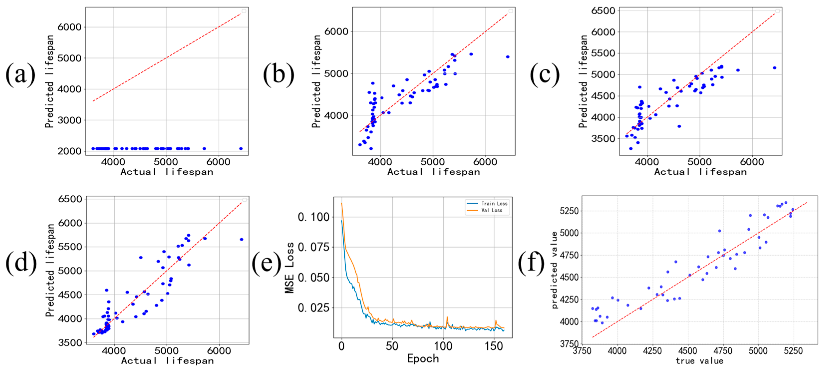
During training, it is crucial to normalize the lifespan labels as well. If only the features are normalized, it will result in a significant difference in the order of magnitude between the features and the labels. The neural network will have difficulty distinguishing subtle differences in the features and will end up with the same predicted value for all cases, as shown in Figure 7a.

If LSTM is not used, and only the simplest BP neural network is employed, the prediction results are shown in Figure 7b. The evaluation index of the training results, RMSE, is 344.71, and the R² value is 0.7225.

If a simple RNN neural network is adopted, the prediction result is shown in Figure 7c. The evaluation index of the training result, RMSE, is 337.60, and the R² value is 0.7339. Since RNN can capture temporal features better than the BP neural network, its performance is significantly better than that of the BP neural network.

As a variant of the RNN neural network, the scatter plot of the final prediction results obtained by training the LSTM neural network and the actual values is shown in Figure 7d. Its ability to capture time characteristics is stronger. The evaluation index of the training result, RMSE value, is 293.31, and the R² value is 0.8097 (the calculation of the evaluation index is in the code, and it is automatically calculated and given after the neural network training is completed). It can be seen that its effect is significantly better than that of BP and RNN neural networks. The scatter points are basically distributed along the diagonal, indicating that the predicted values of the model are close to the actual values.

Mean Square Error (MSE), also known as quadratic loss or L2 loss, is a commonly used loss function in machine learning, especially suitable for regression prediction tasks. MSE is a convex function, which ensures that when using optimization algorithms such as gradient descent, as long as the learning rate is reasonable, it can converge to the global optimal solution. At the same time, since it is a quadratic function, MSE is continuously differentiable everywhere, which is convenient for calculating the gradient and suitable for gradient descent and other optimization algorithms for model training. The gradient of the predicted value with respect to the error is proportional to the error, and the larger the error, the greater the parameter update amplitude. The MSE formula is simple, only requiring the squaring, summation, and averaging operations of the error, with low computational complexity and suitable for training scenarios with large-scale data. The advantages of MSE are that it imposes a greater penalty on large errors, allowing the model to pay more attention to reducing large errors, thereby making the predicted value closer to the true value. At the same time, the smooth and differentiable characteristic makes the model training process more stable and easier to converge. However, it is sensitive to outliers because the squaring operation significantly amplifies the loss of outliers, which may lead to the model over-fitting to outliers and reduce the model’s prediction performance for normal data. The loss function curve during the training process is shown in Figure 7e. It can be seen that the loss fluctuates during the training process and eventually stabilizes within a certain range, indicating that the neural network has successfully learned the features in the data.

Time series often contain cross-period dependencies, and traditional models (ARIMA, simple RNN) are unable to capture dependencies beyond 10 steps due to the problem of gradient vanishing. Time series often have situations where the mean and variance change over time. LSTM dynamically adjusts the gating weights to handle such changes. When the data distribution undergoes a sudden change, the input gate increases the weight of new data and the forget gate quickly clears the old distribution features. LSTM can simultaneously input multiple related sequences, and the gating mechanism automatically learns the temporal correlations between variables. The forget gate assigns low weights to irrelevant variables, while the input gate focuses on the changes in core variables. A multi-layer LSTM can capture short-term fluctuations at the lower level and abstract long-term trends at the higher level. LSTM has demonstrated unique advantages in predicting device lifetimes.

The implementation process of the hybrid model: Firstly, physical modeling was conducted using COMSOL to simulate the chip. Initially, the heat distribution data was obtained. The data was then input into the Weibull–Arrhenius physical model, resulting in the performance decay curve of the chip. The value at which the performance decay reached 20% was taken as a predicted lifetime. The Weibull–Arrhenius model describes the chip performance degradation caused by temperature cycling. Its core lies in the correlation between lifetime and average temperature, and it determines the mode of equipment performance decline. Subsequently, COMSOL continued to perform stress simulation, calculating thermal stress. Through fatigue simulation, the chip’s lifetime under the influence of thermal stress was obtained, and the thermal distribution data and lifetime data were combined into a dataset. This dataset was learned through a neural network LSTM, and the predicted lifetime values were obtained. Finally, the lifespan values obtained by different methods are added together according to certain weights. After extensive data verification, it is empirically determined that a ratio of 0.63:0.37 is more appropriate. This weight is the ratio when both the APE (Absolute Percentage Error) and MAPE (Mean Absolute Percentage Error) values are at their minimum in the experimental results. It indicates that, based on the comprehensive data obtained, this weight is the ratio that, on the whole, makes the predicted results closest to the actual situation. That is:

$$Life=w_1{L}_1+w_2{L}_2$$

(5)

Among them, “Life” refers to the predicted ultimate lifespan, “L₁” represents the lifespan value obtained from the Weibull–Arrhenius model, and “L₂” refers to the lifespan value predicted by the trained LSTM. The weights w₁ and w₂ are 0.63 and 0.37, respectively.

The scatter plot showing the distribution of 50 sets of actual lifespan data obtained through accelerated lifespan testing and the predicted lifespan data obtained using the mixed model is shown in Figure 7f.

The formula for calculating Absolute Percentage Error (abbreviated as APE) can be expressed as:

$$APE=\left|{\displaystyle \frac{{\widehat{y}}_i-y_i}{y_i}}\right|\times 100\%$$

(6)

Here, ${\widehat{y}}_{\mathrm{i}}$ represents the predicted value, while $y_i$ represents the actual value.

Mean Absolute Percentage Error (MAPE): The average value of the APE for multiple predicted samples. The formula is as follows:

$$\mathrm{MAPE}={\displaystyle \frac{1}{n}}\sum _{i=1}^n\left|{\displaystyle \frac{{\widehat{y}}_i-y_i}{y_i}}\right|\times 100\%$$

(7)

It is commonly used to evaluate the overall accuracy of a prediction model and is a classic indicator for measuring prediction accuracy.

Among these 50 sets of data, the maximum absolute percentage error is 8.51%, and the average absolute percentage error is 3.07%. This meets the requirement that the overall error is less than 10%.

Weibull–Arrhenius Model: This model reflects the impact of heat accumulation during the operation of the equipment on its various performances, which in turn leads to the equipment’s wear and tear. By establishing the connection between heat and chip performance degradation, the performance decay of the chip can be obtained, thereby determining the service life. COMSOL Fatigue Simulation + LSTM: This method reflects the different thermal expansions caused by different heating, cooling, and heat transfer during the equipment’s operation, thereby generating thermal stresses. Considering the equipment’s ability to withstand stress, the service life value can be obtained, and it is learned using the LSTM neural network. Hybrid Model (Combining the Above Two Models): The Weibull–Arrhenius model directly reflects the impact of heat on the equipment’s performance loss. COMSOL Fatigue Simulation + LSTM Neural Network takes into account the possible damage to the equipment’s structure caused by stress based on heat. Combining these two methods achieves complementary advantages, enabling a more comprehensive and accurate consideration of various factors when predicting the lifespan of GaN power devices, significantly improving the prediction accuracy. This fully demonstrates the effectiveness and superiority of integrating different types of models, providing a more reliable and precise solution for accurate prediction of GaN power device lifespans, and helping to more reasonably evaluate the reliability and lifespan of devices in practical engineering applications.

4.

Optimized direction

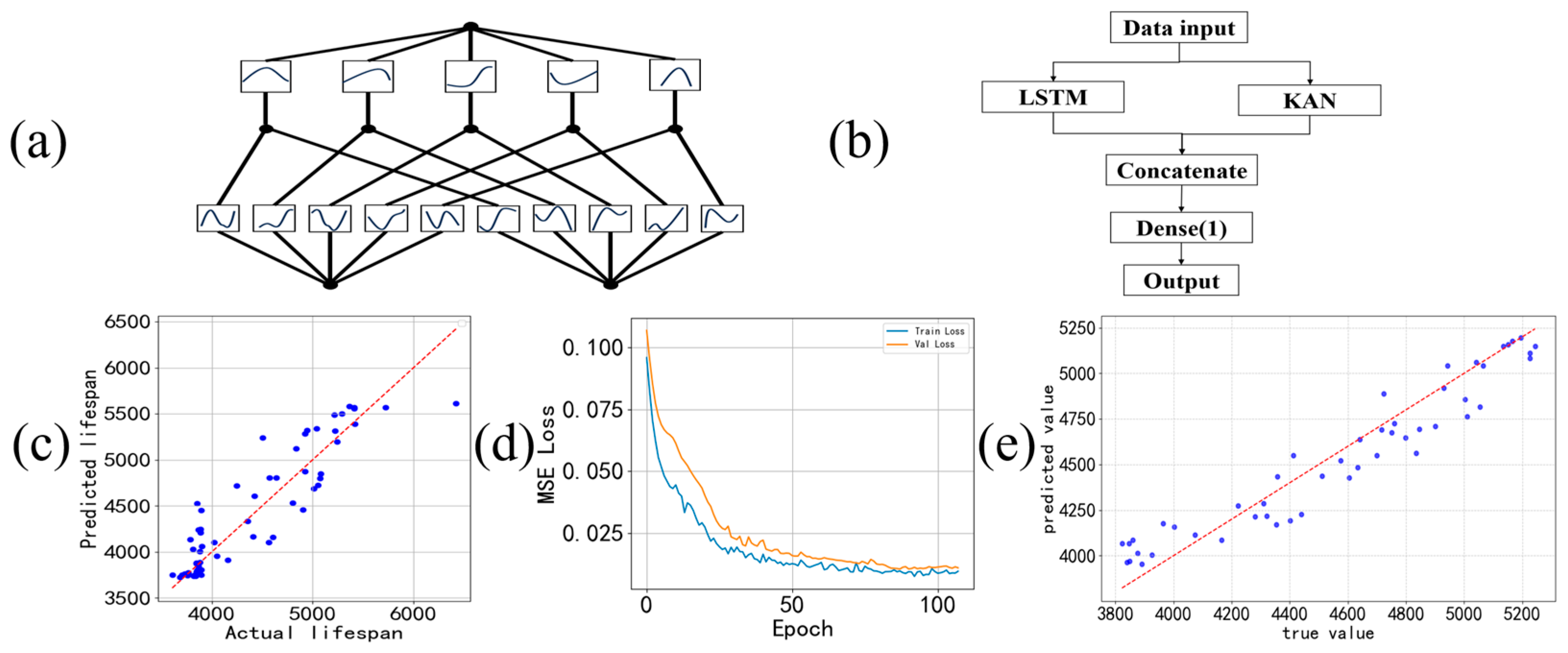
KAN (Kolmogorov-Arnold Network) is a new type of neural network structure based on mathematical representation theorems. It replaces the activation function of traditional neural networks with multiple learnable unary nonlinear functions, thereby achieving efficient approximation of any continuous multivariate functions. Its structural schematic diagram is shown in Figure 8a. These unary functions are often constructed using B-spline functions because they possess advantages such as smoothness, local controllability, and good differentiability. By combining KAN with LSTM, the ability of LSTM to capture temporal features and the advantage of KAN in capturing complex nonlinear relationships of input variables can be fully utilized, enhancing the model’s expressive power and prediction accuracy. The hybrid model structure is shown in Figure 8b. The input data is simultaneously passed into the LSTM and KAN branches: LSTM processes the time series sequence through the gating mechanism (input gate, forget gate, output gate), and outputs a vector containing temporal dynamic features; KAN maps the input features to nonlinear feature vectors through the B-spline function layer. The two outputs are concatenated through the Concatenate layer, and finally, the prediction result is output through the fully connected layer. During training, the temporal features of LSTM provide a “dynamic background” for KAN, and the nonlinear features of KAN supplement “static correlations” for LSTM. The two update parameters through back propagation collaboratively, improving the model’s adaptability to complex data.

The RMSE value obtained from the training of the KAN-LSTM neural network is 281.29, and the R² value is 0.8152. The training results and loss function are shown in Figure 8c,d. The MAPE value obtained by comparing the predicted life with the actual life after combining the prediction results of KAN-LSTM with the COMSOL simulation results is 2.58%, and the Max APE value is 6.42%. The prediction results are shown in Figure 8e. It can be seen that the prediction accuracy of the KAN-LSTM neural network is improved compared to the pure LSTM neural network. However, the data complexity used in this paper is not high, so the improvement in the prediction accuracy of the life of the KAN-LSTM neural network compared to the LSTM neural network is not obvious. With the increase in data complexity, the KAN neural network can leverage its better ability to capture nonlinear relationships to make the KAN-LSTM neural network exhibit superior prediction capabilities. In the future, it can be used as an optional optimization solution.

4. Conclusions

This study presents a hybrid framework integrating finite element simulation and deep learning for accurate lifetime prediction of GaN power devices. By leveraging COMSOL Multiphysics to simulate thermomechanical behavior under varying operational conditions, key degradation indicators such as thermal cycling and stress concentration are effectively extracted. These features are then used to train an LSTM neural network capable of modeling the temporal degradation patterns of GaN devices. This method was proposed based on the consideration that conducting a large number of practical experiments requires a significant amount of time and resources, which is difficult to achieve within a short period of time. Therefore, it was decided to adopt simulation experiments to expand the sample size. Under limited conditions, this is a feasible approach. If sufficient experimental data can be obtained later, it can be directly used to replace the simulation data, thereby obtaining more accurate prediction results. This work is conducive to promoting the development of predictive maintenance and reliability engineering for next-generation power electronic devices based on gallium nitride.