Predictive Navigation of Mobile Robots in Dynamic Environments: A UKF–APF Approach

Abstract

Human behavior when navigating a dynamic environment relies on predicting the near future that describes immediate states of moving objects based on their current trajectories. Mobile robots, instead of using a similar approach in many cases, rely only on feedback from the current moment in time, which can result in close encounters with obstacles, leading to trajectory instability due to a strong control signal coming from avoidance algorithms. This paper presents an approach that uses predictive control based on dynamic environment estimation performed by an Unscented Kalman Filter. The predictor analyzes trajectories of nearby objects and assesses the possibility of collision or close encounter. This introduces an additional control signal integrated into the Artificial Potential Fields algorithm, which helps to reduce rapid changes in the control signal, in effect smoothening the robot’s trajectory, as well as reducing the likelihood of dangerous situations happening.

1. Introduction

There is a consistent trend of providing machines, especially robots, with increasingly complex control systems whose primary purpose is to make them work more safely and more efficiently. Many of those solutions are based on the behavior of living organisms: Genetic Algorithms, Ant Colony Optimization, Fuzzy Logic, or Neural Networks, to name just a few, are all inspired by how nature handles complex information processing.

Despite extensive research and many known successful applications, a number of commercially available autonomous mobile robots with well-developed safety systems are missing one crucial aspect of how living organisms handle real-time feedback during movement: prediction. To understand the idea, consider walking through a tech fair. Every individual moves independently, often in an unpredictable manner, yet despite a highly dynamic environment, collisions are rare occurrences. It is possible because every agent in this environment is actively predicting short-term trajectories of others and adjusting its planned trajectory accordingly based on sensory feedback. This decentralized prediction-based navigation allows smooth and efficient flow without global coordination—a key principle worth translating to robotics.

This behavior can be reproduced to a certain degree within constraints of a digital navigation system through the use of UKF-APF algorithms in tandem. A state estimator can be used to evaluate the current conditions of other agents present in the environment. Connected with a predictor algorithm, it can be used to assess the immediate future of the workspace, reproducing expectations a person has regarding their surroundings, which hints at what trajectory should be taken to safely move towards the target. APF also recreates basic assumptions of human navigation: move towards the target, move away from obstacles. As such, it can be easily integrated with a predictor algorithm through the introduction of additional forces. Utilization of distribution described through sigma points is also possible as a means of fine-tuning the control system, but it is out of the scope of this work and will be explored in the future.

Prediction-based navigation for robots has been widely studied, with several approaches proposing to integrate prediction into the control loop. The authors of [1] provided a detailed formulation of predictive control for mobile robot navigation, where the position described in time is not used as a constraint, but another degree of freedom available to the controller instead. This way, depending on the situation, the controller is able to focus on maintaining safety and feasibility of the navigation task instead of enforcing a vector of consecutive positions described in function of time. The downside of this approach is that the environment is assumed to be static, limiting its application in dynamic conditions. In ref. [2], a similar problem of predictive control is described, but the approach is more focused on the dynamics of the robot and exploring optimal control in an environment with unknown elements. The authors introduced compensation of stochastic disturbance, which increases robustness, but again, it assumes the environment to be static in each planning cycle. This approach will work well in static or low-dynamic settings, but might struggle in highly dynamic conditions. The authors of [3] presented an approach expanded to control a fleet of wheeled mobile robots, where predictive control helps with maintaining formation. Their work shows that introducing a predictive control approach for a robot fleet allows for achieving visibly better navigation quality when using time constraints, as well as keeping formation with non-omnidirectional robots. The downside of this approach is the usage of shared information, which requires a stable flow of detailed information, an assumption that is not always feasible. In ref. [4] the authors focus on the analysis of predictive control stability in the presence of unknown disturbances and their effect on path following precision. The presented approach increases the robustness of the system, but it focuses on a single agent operating in the environment, not exploring the case of a dynamic environment. The authors of [5] present an approach to minimize wheel slip through analysis of forces that are required to adhere to preemptively assumed kinematic constraints through a nonlinear MPC framework. Their work addresses low-level motion feasibility but does not address global navigation or dynamic obstacle avoidance.

Recent research has shifted towards AI-based navigation for autonomous robots, which is also implemented in the context of predictive control. The authors of [6] proposed transformer-based prediction network describing spatio-temporal relations between robot and other dynamic agents, producing multimodal future distributions. It improves long-horizon prediction accuracy compared with classical kinematic models, but requires a large amount of resources for training as well as for real-time computing, limiting usability on embedded systems. Reinforcement learning has also been used to augment the capabilities of the APF algorithm. For instance, results presented in [7] used a potential field as a reward function, trying to improve convergence and escape local minima. This approach significantly increases the robustness of the system, but similarly to above, it requires a large amount of resources for training and additional computational time for implementation. There can also be seen examples of multi-sensor fusion being used for robot control. In refs. [8,9] authors present an IMU connected with LiDAR for increased robustness and uncertainty estimation of the localization system. This set of sensors is often used for embedded systems, as it does not require a significant amount of computational resources, but low-cost IMUs require multiple levels of data filtering and conditioning to achieve good quality of information [10].

This work presents the usage of classical methods for UKF-APF predictive control with LiDAR-based feedback, with a focus on addressing problems caused by the generic APF controller in a dynamic environment. This setup allows for estimating the state of all dynamic obstacles present in the robot’s workspace through the UKF algorithm. The implementation of chosen LiDAR-only feedback for detecting obstacles, instead of introducing a camera for additional data, aims to reduce the computational resources needed for achieving functionality and make it applicable for typical embedded systems. Described algorithms, apart from being tested in the Matlab environment, were also translated to C using the Embedded Coder toolbox and designed in such a way to maintain good practices known from most widely used coding standards like MISRA C or ASIL. They were then programmed and executed on STM32F407G Discovery Board to verify feasibility of using them on commercially available microcontrollers, which would serve as starting point of implementing it on physical system.

2. Motion Controller

The proposed motion control system is based on the Artificial Potential Field algorithm. First presented in [11] is one of the most popular approaches for obstacle avoidance and motion control. Currently, many different modifications and applications can be found in the literature. The authors of [12] presented an interesting method based on deterministic annealing to look for possible local minimum areas before the robot comes into them and steers away, saving time and energy. The downside of this approach is that, by the nature of deterministic annealing, it might perform worse in a dynamic environment, while reaching the global optimum is not guaranteed. In ref. [13] Ant Colony Optimization metaheuristic-focused approach is presented, significantly reducing the typical amount of iterations required for ACO-based path planning, at the same time lowering the median path length through the usage of APF. The limitation of this method is the significant computational overhead required by the metaheuristic component to converge, as well as the loss of determinism. In ref. [14] authors presented a robot fleet control system based on the APF approach to maintain formation and safe distances between agents when avoiding obstacles. While it shows great performance with local path adjustment in the scale of the fleet, some issues related to oscillations of the control signal were not addressed explicitly, and stable communication between agents is required for the application.

In the scope of this work, the APF algorithm is used as a motion controller that focuses on obstacle avoidance. The basic data input for the algorithm is feedback from the LiDAR scanning the robot’s immediate surroundings, as well as information about the robot’s localization and the current target, ensuring the robot will attempt to achieve its target. Apart from those calculations, the robot will perform the prediction of the obstacle trajectory in the immediate future based on the UKF estimation, so no communication with other agents is required.

2.1. UKF State Estimator

The unscented Kalman Filter described in detail in [15] alongside the Extended Kalman Filter is one of the most commonly used state estimators for nonlinear systems. A discussion about the pros and cons of these two algorithms and how they compare with each other has been ongoing for many years, with no clear winner. The difference in precision and computations required depends on the use case [16,17,18,19]. The authors decided to choose UKF because of how the Unscented Transform represents data. The Gaussian distribution of the parametric estimate is represented by a set of Sigma Points, which in essence defines a one-sigma area around the estimated state. This representation is more intuitive to use in connection with other algorithms related to path planning than the covariance matrix in the EKF approach, and will provide a basis for future work regarding finer predictive mobile robot control.

For obstacle state estimation, the most common dynamic representation in a 2D environment has been assumed, where the state vector consists of 9 variables:

$$\chi ={[x,\dot{x},\ddot{x},y,\dot{y},\ddot{y},\theta ,\dot{\theta },\ddot{\theta }]}^T$$

(1)

This vector represents the full state vector that will allow fine tracking of the obstacle’s dynamic state and will provide input for further calculations. For this application, UKF was modified compared with its basic form, which can be found in [20], because it caused problems when estimating orientation. Depending on how motion controllers are coded, orientation is expected to be limited to $(-\pi ,\pi )$ or $(0,2\pi )$ range. In Figure 1a comparison can be seen between simply limiting orientation value and implementing additional logic within UKF to handle overflow case. It can be seen that if it is not properly addressed, UKF will treat it as a sudden change in the measured state, leading to errors in the following velocity and acceleration estimation.

To address this problem, a phase unwrapping algorithm has been added inside UKF code logic to maintain $(-\pi ,\pi )$ orientation range that adheres to the notation of atan2 function (Algorithm 1). This approach had been analyzed in [21] and in this work was implemented for 3D UKF handling 3 degrees of freedom for the angular dynamic state with a single measurement describing the current orientation:

Algorithm 1 UKF angle overflow handler.

1: if $abs(y-\theta )>1.5\pi$ then 2:     if $\theta <0$ then 3:         $\theta =\theta +2\pi$ 4:     else 5:         $\theta =\theta -2\pi$ 6:     end if 7: end if

where:

• $\Theta$—3D angular dynamic state $\Theta$ = [$\theta ,\dot{\theta },\ddot{\theta }$],
• y—measurement of current orientation.

  The general idea is that angle measurement y uses atan2 notation, which may cause discontinuity when going from $\pi$ to $-\pi$. This will cause a false-positive occurrence of high velocity between two iterations of UKF, resulting in a significant following error. The correctness of the data is verified by the first condition, where the absolute value of the difference is compared. The value used for comparison should be big enough that a quick change in orientation detected by sensors will not trigger the algorithm, but accordingly smaller than $2\pi$, so it could be described as follows:

$$(BPC,2\pi -BPC)$$

(2)

where $BPC$ stands for Biggest Possible Change in orientation, which results from the dynamics of present dynamic obstacles as well as the scheduling rate of the algorithm, e.g., if based on knowledge about the environment where the robot works, it can be said that in a single iteration of the control system, a detected obstacle would not turn for more than 3, then $BPC=3$.

When the function is triggered, it will change the internal value of the estimated value, which then will be used during the innovation stage of the algorithm with the same measurement used in the condition. With this approach, no sudden change in the difference between measurement and estimated orientation will occur, effectively maintaining the high accuracy of the estimated state.

2.2. Predictor Algorithm

The UKF algorithm calculates an estimated state of all obstacles without using any global data or knowledge about their kinematic structures. This property makes the presented approach highly reusable and robust in terms of possible applications. The estimate is used as the main input for the collision prediction stage of the navigation system, which, based on the data, verifies if navigation should proceed in the current state or adjustments need to be made. The prediction algorithm is separated into three stages, which will be described in detail below.

In the first stage, predicted trajectories of obstacles and the robot are calculated. In case of obstacles, the current estimated state is expanded upon to N discrete steps into the future based on its position, linear velocity, and angular velocity. Accelerations are not taken into consideration because obstacles are assumed to be moving with constant velocity when not turning, and small values coming from virtual measurement inaccuracies and the UKF itself contributed to the prediction being burdened with bigger errors than when using only velocities.

In case of prediction of the robot’s state, there are two tested approaches: a theoretical straight-to-target prediction, and one that calculates the same way as obstacle predictions. The first option creates a series of points that are directed towards the current target, taking into account only the current velocity of the robot. The idea behind it is that when the robot changes direction to go around a moving obstacle, then its predicted trajectory based on estimation will not be on a collision course anymore, which will cause it to get closer to the obstacle and make trajectories collide again. The described behavior is close to a two-state regulator, causing the robot to oscillate. Results of using both approaches will be presented in the next section.

The second stage is checking whether a collision may occur if the current trajectories are maintained. For each point of the robot trajectory prediction, the distance from successive points of the obstacle trajectory is calculated. If the distance is smaller than a chosen safety margin, which is assumed based on the size of both the robot and the obstacle, then the point is marked as a potential collision.

The sections of both trajectories where collision may occur are then processed in the third stage. There are many approaches to avoiding the collision, such as speeding up, slowing down, or going around. For the scope of this work, a robot has a constant velocity assumed; as such, the focus is on the going around strategy. To perform it, information about the side from which the obstacle is coming is required. To determine it, a linear function based on a segment of the robot trajectory is created, which is described in Algorithm 2. Depending on the slope of this function and whether its value at the same X coordinate as the point taken from the obstacle trajectory is bigger or smaller, the direction from which the obstacle is approached can be calculated.

R denotes x and y coordinates of 2 points of robot trajectory in segment where collision may occur. O denotes a point from the obstacle’s predicted trajectory in which a collision may occur. $X_{dir}$ determines if the robot is currently going in a positive or negative direction of the global X axis. In line 8, it is being verified whether the point O is above or below the line created from the points R. Based on it and knowledge of which direction the robot is going, it can be determined if the obstacle is approaching from the left-hand side or the right-hand side.

Algorithm 2 Check obstacle side.

1: $a={\displaystyle \frac{R(2,2)-R(1,2)}{R(2,1)-R(1,1)}}$ 2: $b=R(1,2)-a·R(1,1)$ 3: if $R(2,1)>R(1,1)$ then 4:     $X_{dir}=1$ 5: else 6:     $X_{dir}=-1$ 7: end if 8: if $O\left(2\right)<=a·O\left(1\right)+b$ then 9:     if $X_{dir}==1$ then 10:         $O_{side}=L$ 11:     else 12:         $O_{side}=R$ 13:     end if 14: else 15:     if $X_{dir}==1$ then 16:         $O_{side}=R$ 17:     else 18:         $O_{side}=L$ 19:     end if 20: end if

2.3. APF-Based Motion Controller

As mentioned at the beginning of the section, the Artificial Potential Fields algorithm was chosen as a basis for the motion controller. This approach is simple to implement, robust, and easily modifiable, be it on the design level or during runtime, making it a popular choice. The controller used in the presented work makes use of the superposition of three forces:

• attraction to the target
• repulsion from the obstacle
• repulsion from the predicted collision

Attraction to target is based on current orientation of the robot and its angular distance from the target. Its value is calculated using the atan2 function with post-processing consisting of scaling the force and forcing a minimum amplitude.

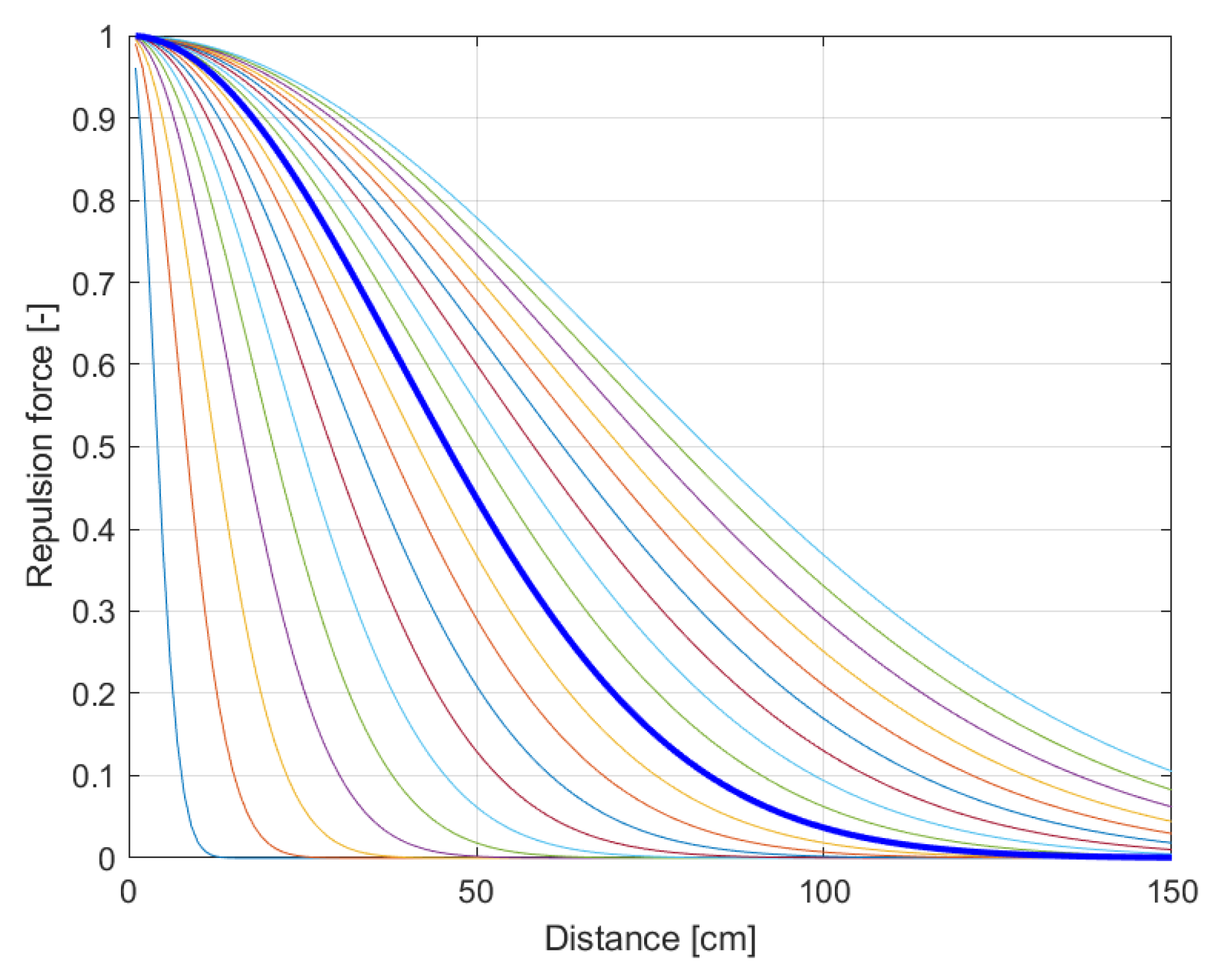
Repulsion from obstacle is force that is responsible for avoiding crashes with obstacles, both static and nonstationary. The usual practice when designing this force is using an exponential function with the distance from the target as an argument. In this work the equation of the function, based on previous simulations, was chosen as follows:

$$Rep=e^{-({\displaystyle \frac{d}{55}}{)}^2}·sign\left(sin\left(a\right)\right)$$

(3)

where $Rep$ is the repulsive force, calculated separately for each LiDAR measurement point, d is the distance from the detected point, and a is the angle to the detected point relative to the front of the robot. The Signum function is used to determine whether the robot should turn left or right to avoid an obstacle. The parameter in the denominator was chosen to be 55 based on experiments on the APF motion controller conducted in [22]. Presented function was checked for multiple values of the parameter to check how the curve would be changing, what can be seen in Figure 2. The value chosen reflects the limited dynamics of the simulated robot, which requires initiating avoidance maneuvers in advance.

Repulsion from predicted collision is scaled in a similar manner as a repulsive force, but a linear function was chosen instead. The equation for this component of the steering is as follows:

$$P_{steer}={\displaystyle \frac{40P_{dir}}{P_{dist}+1}}$$

(4)

where $P_{dir}$ fulfills the same role as the signum function in the case of the previous repulsive force and represents the direction from which the obstacle is approaching. $P_{dist}$ is the distance from the predicted collision point, responsible for scaling the force. Parameter 40 in the numerator was chosen empirically based on the robot’s behavior in the simulation. Low values did not contribute enough to the overall steering force, which limited the usefulness of the modification, in general, while high values caused the robot to instantly achieve the maximum permitted angular velocity, which generated problems with trajectory continuity and would cause high mechanical wear and slip if tested on a physical system.

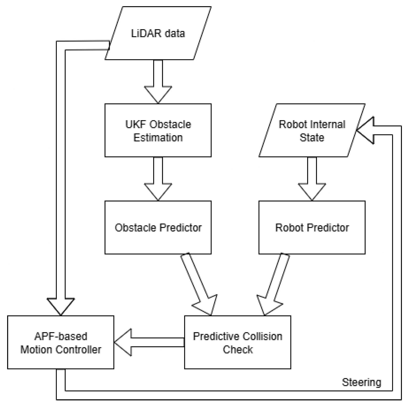
The full data flow of the algorithm described above can be seen in Figure 3. In this work, the robot is assumed to have objective knowledge about its own state. In real applications, it should be estimated as well, but here, to reduce degrees of freedom for developing motion control, this simplification was adopted.

3. Experimental Results

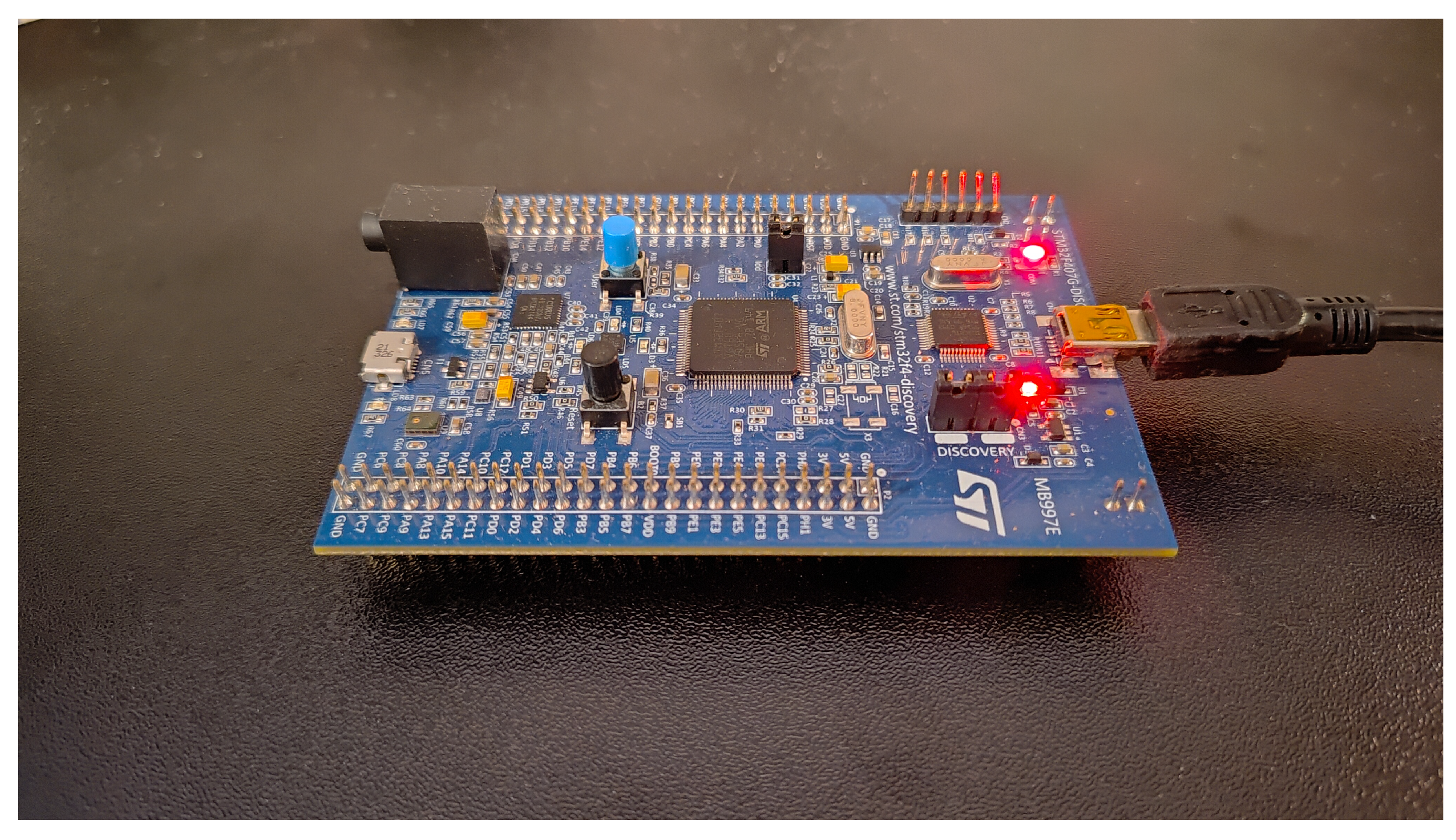
To verify the proposed algorithms, all the presented solutions were implemented in a simulation project prepared in a Matlab environment. The project includes dedicated libraries for generating a dynamic environment, providing sensor feedback that includes measurement error as well as control robot mechanics. Simulations were performed on a machine running Matlab 2022b with Intel i3-12100F CPU and 32 GB 4800 MHz RAM. Because of authors’ good experience with specialized mobile robots that are based on ST microcontrollers, presented algorithms were also tested on a discovery board equipped with STM32F407G controller (Figure 4) that uses 8 MHz clock. To translate the code, MATLAB Coder toolbox was used, running generation supporting ARM Cortex-M systems and full MISRA compliance with no optimization flags or other preprocessor directives.

3.1. Simulation

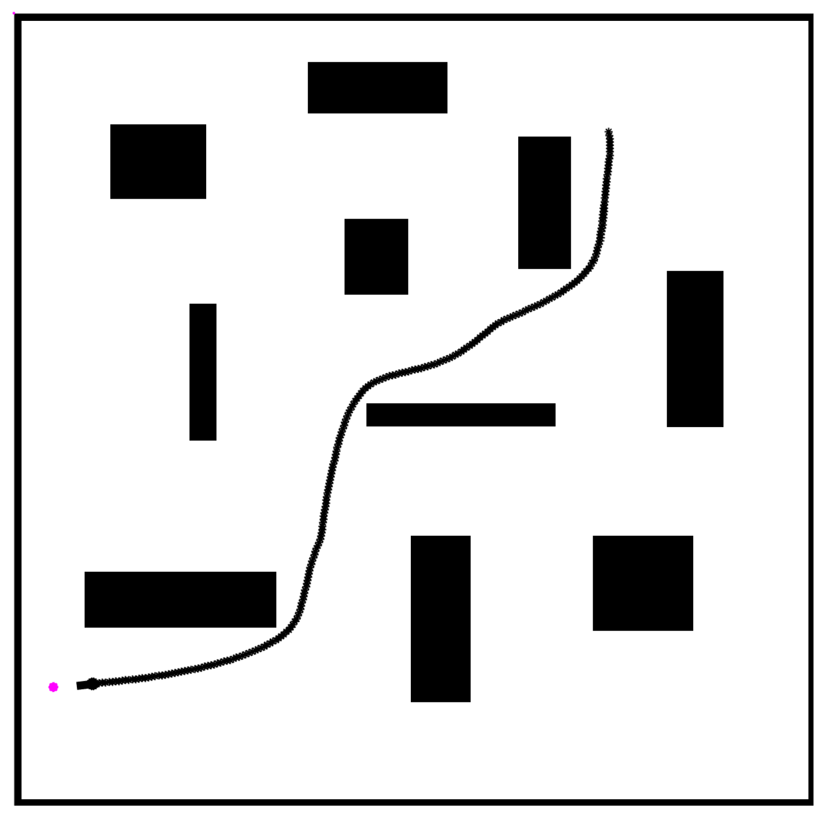
Initial verification of the presented approach was conducted to check if the APF motion controller algorithm works correctly. To ascertain it, a testing environment with static obstacles was prepared. As will be shown in later examples, using only the APF controller might cause problems when the robot finds itself in the immediate surroundings of a dynamic obstacle, which will be resolved through the use of the predictor algorithm. As seen in Figure 5, the robot successfully traversed the environment with static obstacles and reached its target.

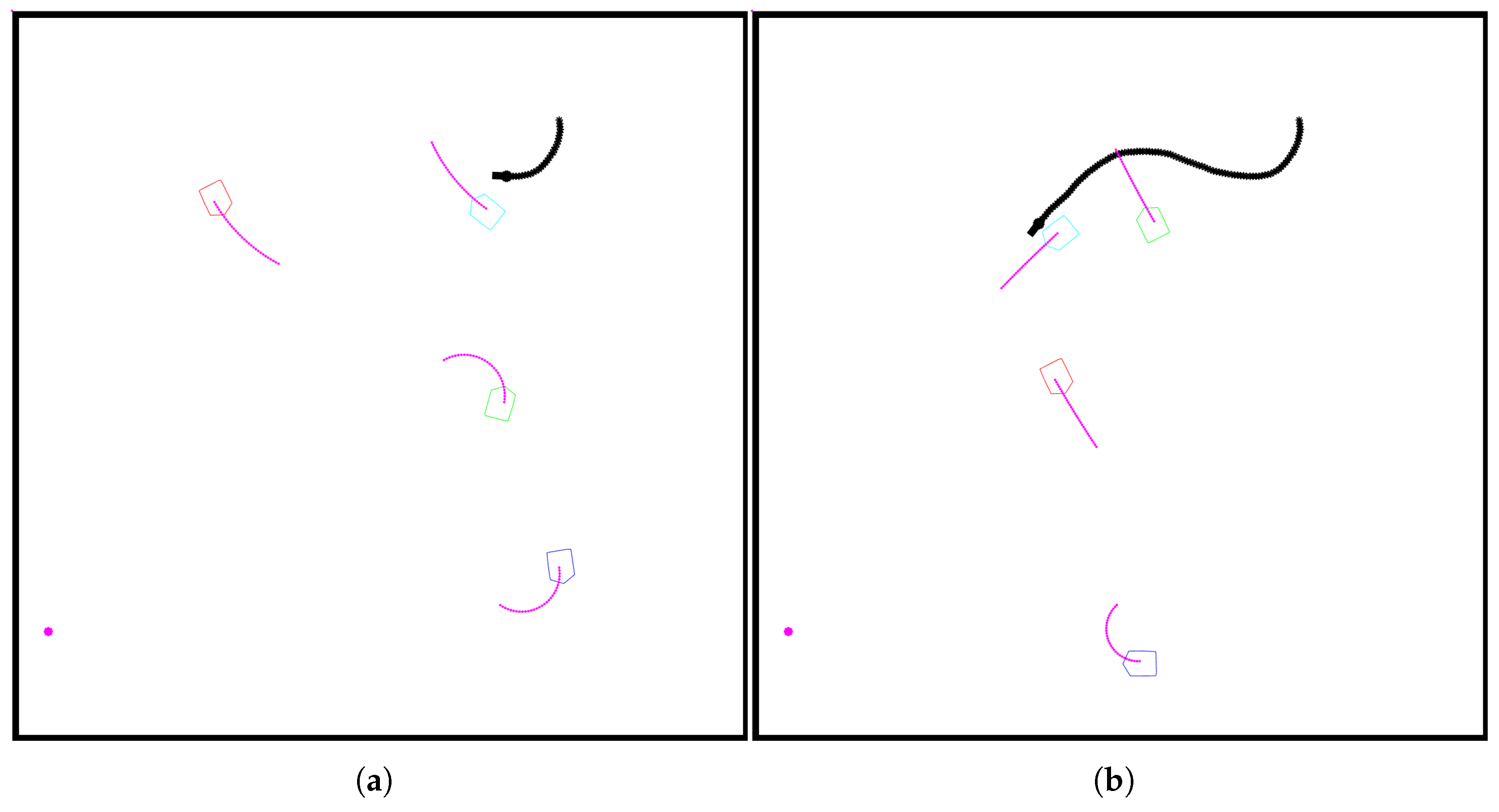
The next step of verification involved running the robot in a dynamic environment without the predictor part of the controller online. All obstacles present in the workspace are moving with constant velocity and have a constant turning rate, with magnitudes similar to those of the robot. The results can be seen in Figure 6. In the figure colored polygons denote dynamic obstacle and purple lines represents prediction of movement. The presented situation is an edge case that was specifically prepared to depict the main weakness of typical controllers working without a predictive component. When the robot and the obstacle met, they started following each other. While the obstacle was moving independently without any safety system maintaining distance from other obstacles (robots), the robot was trying to orient itself towards the target, while the safety system was ensuring that no collision would occur. The result is very specific and can be called another type of local minimum, but at the same time, it represents a situation that might occur when dealing with typical real mobile robots. Certainly, this sort of situation will not last indefinitely like an actual local minimum, but for a significant amount of time, the robot will be staying in a highly unpredictable state.

This problem can be addressed by using a predictor controller that will calculate the most probable trajectory of the obstacle based on its estimated state and change the robot’s steering accordingly. As mentioned before, two possible implementations of the predictor algorithm were considered. The first approach is a more intuitive one, as it uses the same predictor algorithm that was applied for obstacles. 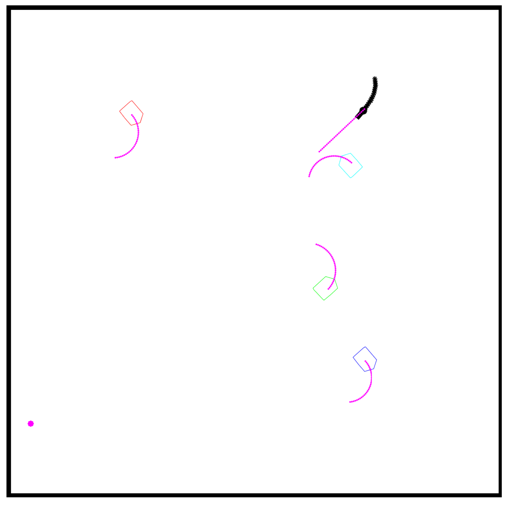Based on the estimation of the robot’s current position and velocities, a simple prediction n step into the future is made. Another approach for predictor controller is to calculate a theoretical linear prediction, which assumes that robot can travel towards its current target unobstructed and a bee-line manner. Both of those methods require overlapping with the obstacle trajectory to occur in order to trigger an avoidance maneuver. This creates a possibly dangerous edge case, in which the obstacle is rotating and its trajectory will overlap with the robot’s only when the two are already close to each other, as shown in Figure 7. It is difficult to predict such a situation early enough without communicating with the obstacle, and for the scope of this work, the robot’s safety at such moments will be left to standard avoidance movement created by APF’s repulsion force.

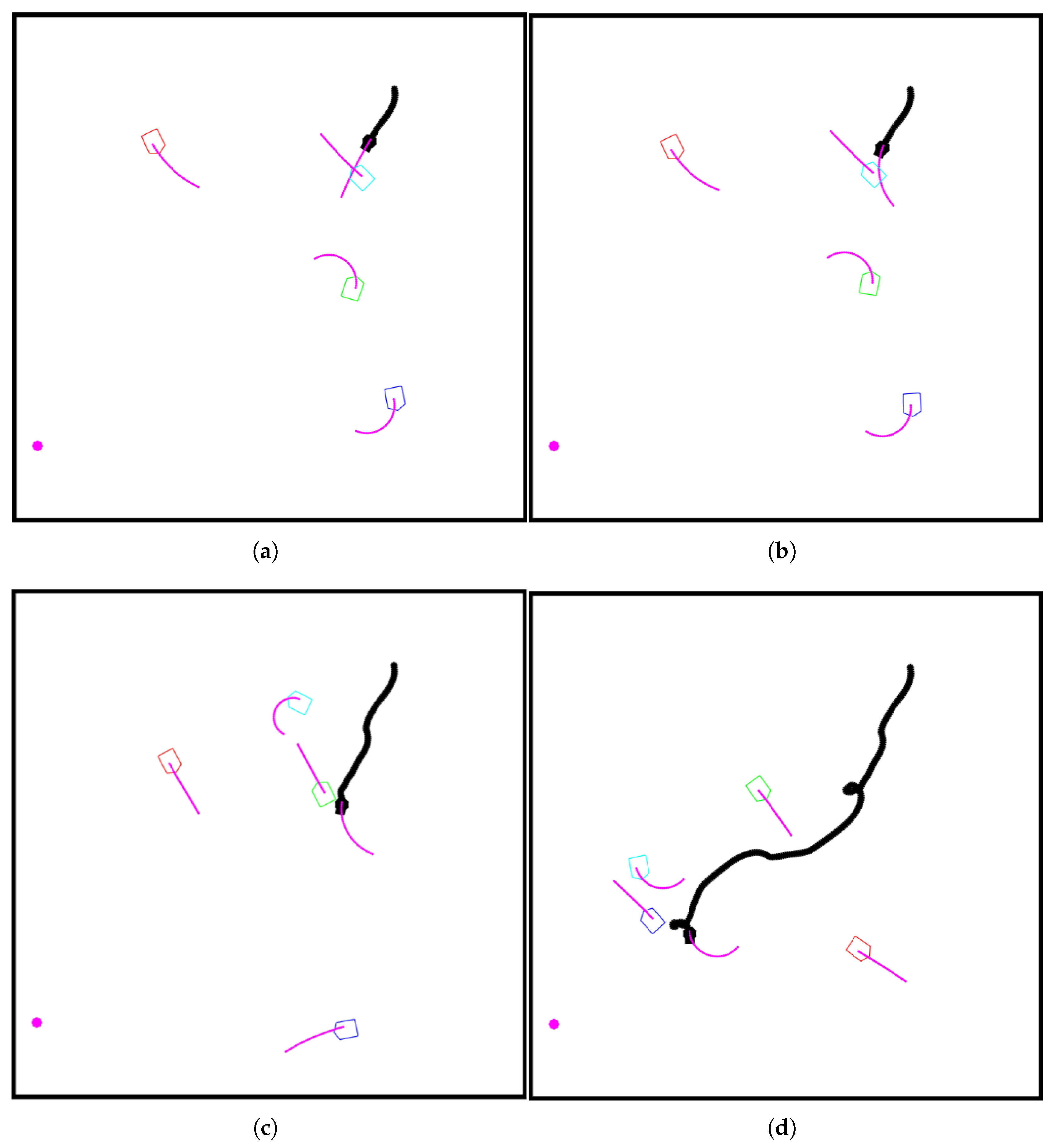
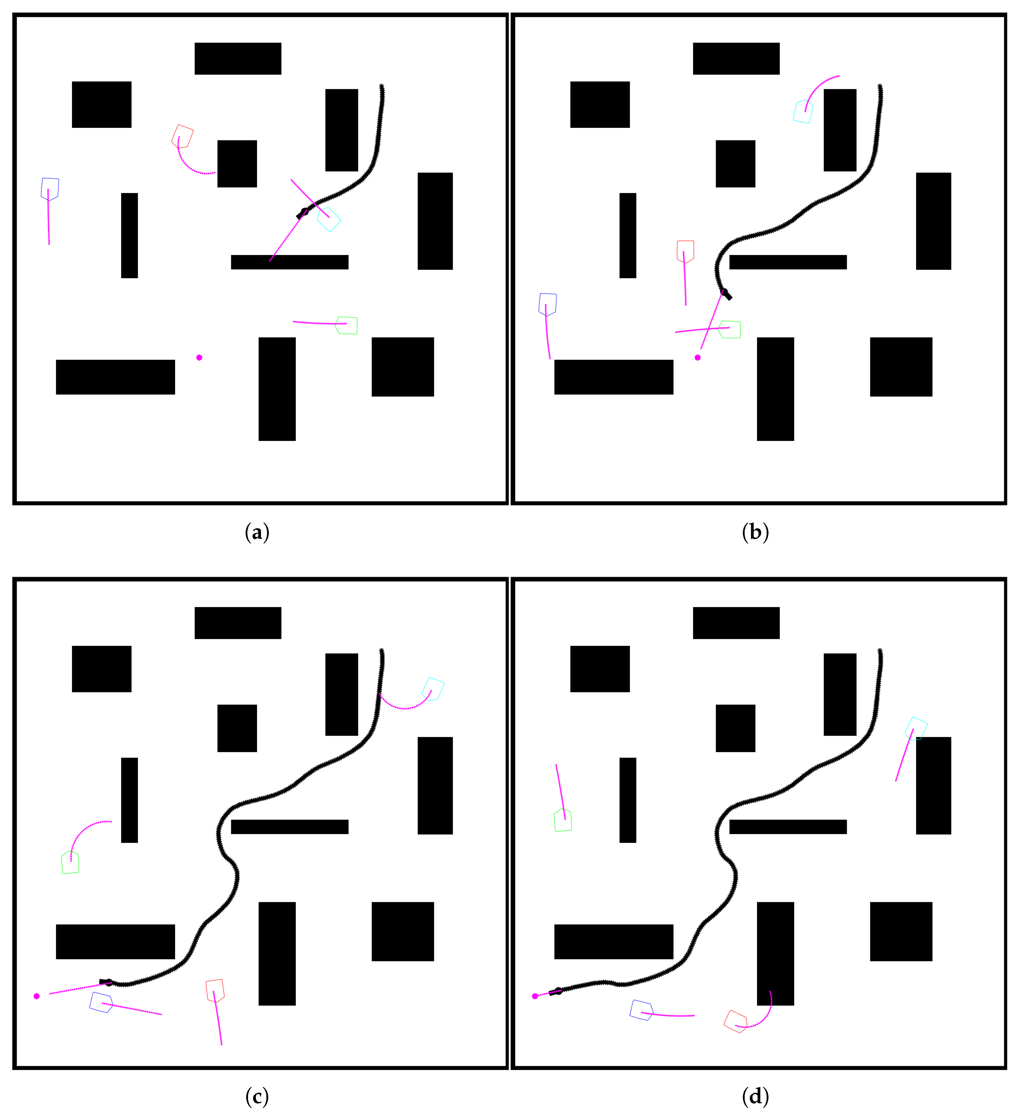
The results of using first approach can be seen in Figure 8. The top pair of Figure 8a,b presents two consecutive time steps, where it can be seen that the prediction of the robot’s movement changed significantly due to its turning. The turning in one hand is caused by the standard repulsive force from APF, but on the other is also caused by the predictor motion controller, which detected the possibility of collision when calculated trajectories are maintained and ordered the robot to turn left in this particular case. In the next time step, when the predictor controller is again checking for possible collision, the predicted trajectory of the robot has already changed due to the previous steering. Because of it, in the current time step, no collision is detected anymore, and as such, the robot will start turning right again because of the attraction force towards the target. The situation that will follow can be seen in Figure 8c. Through the addition of a predictor to the motion controller, the robot will be able to go around the obstacle, and it will do so in close proximity to it. A less desirable situation can be seen in Figure 8d, where the robot will start to make circles at a place. It is presented more as a curiosity because it is unlikely to transpire in case of physical systems, but this situation, in essence, can be easily observed. Most commercial physical systems that authors have experience with in case of very close encounters will start moving around in place, which is caused by the reception of steering signals with rates and magnitudes greater than the actuators, given the system’s inertia, are able to execute. Usually, directly after such a situation occurs, an error flag will be raised and the robot will require the operator’s attention before being able to operate again. A simulation does not have those physical constraints, and no such flag is simulated; as such, a robot starting to dance in place might not be fully detached from a real-life situation when looking from the perspective of the cause of the issue.

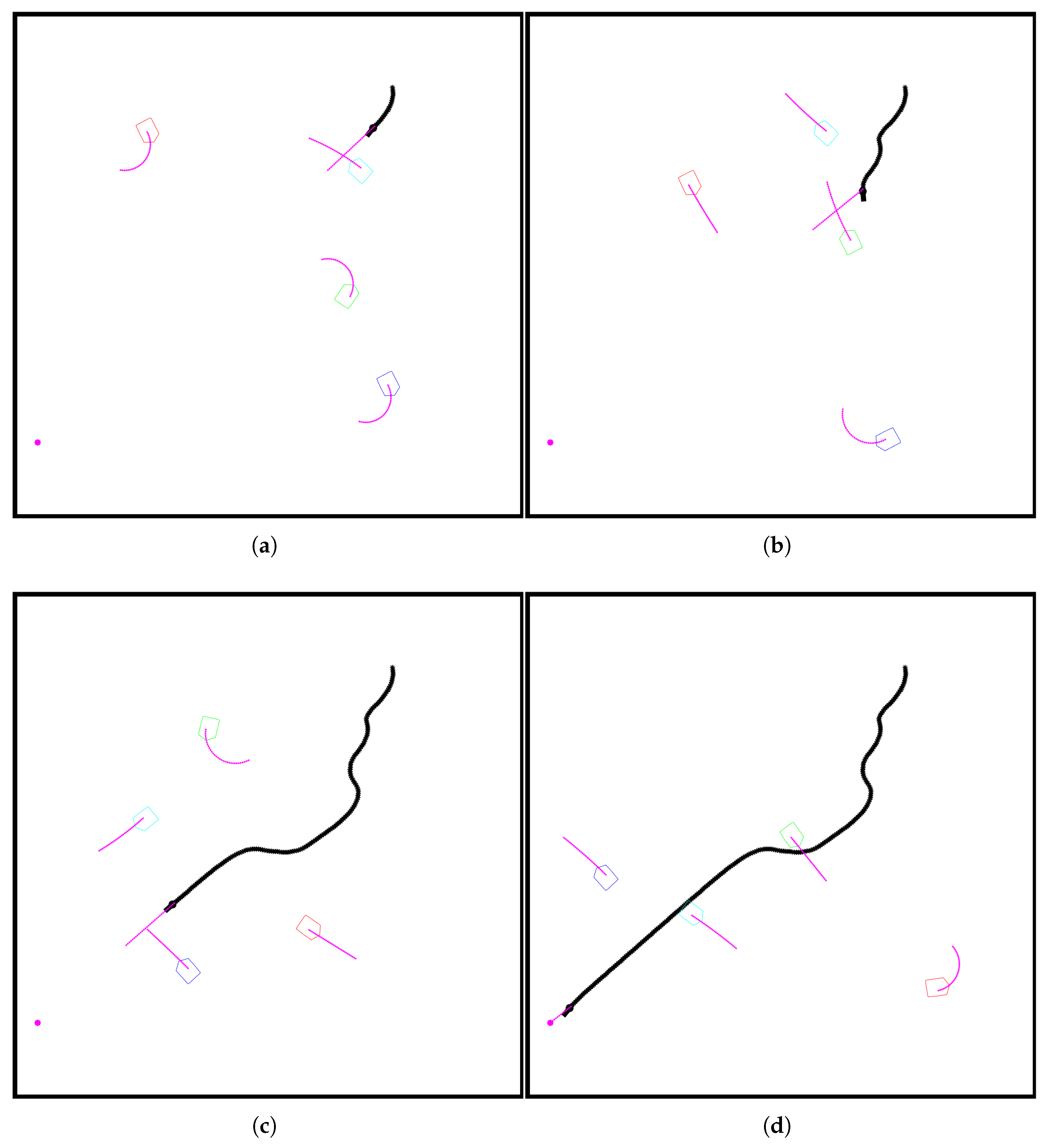
The effects of using the second approach can be seen in Figure 9. Figure 9a shows the moment before the robot starts the avoidance maneuver for the first obstacle. When comparing it with Figure 9b, which is before the second maneuver, it can be seen that while the distance from the obstacle in both cases is similar, the robot orientation has changed earlier in the second case. This is because in the first case, the moment presented is just after the obstacle finishes turning, and only now is on a collision course with the robot, thus the robot started avoidance movement later. Figure 9c can be used to compare avoidance radii-when a collision course was detected earlier, the robot naturally started maneuvering in advance. The same subfigure presents a moment when the predicted trajectories of the robot and the blue obstacle started overlapping. Figure 9d shows that despite it happening, the robot’s trajectory remained unchanged. This is because, as described before, the algorithm is analyzing predictions in a certain range, both physical and temporal. If trajectories are overlapping, but their distance on the time axis is big enough, both objects will not happen to be in each other’s close enough vicinity that would justify commencing a maneuver.

For the next experiment, an environment with both static and dynamic obstacles was prepared. The results can be seen in Figure 10. In Figure 10a, a robot is proceeding with a light maneuver to maintain a safe distance from the first dynamic obstacle. In Figure 10b, the robot can be seen already going around the second obstacle after the system detected a possible collision. In Figure 10c, another minor change in trajectory is required to get around the third obstacle. It is important to know that the avoidance part of the APF controller does not differentiate between the detection of static and dynamic obstacles, so in this case, the robot will have a tendency to get closer to the dynamic one, as static ones are targeted by more LiDAR rays. Differentiating between them to keep a smaller distance from the static obstacle, which is a safer option, will be the subject of future work.

3.2. Embedded Evaluation

Time of execution in an embedded system was tested using four data sets with 30-step predictions exported from a Matlab simulation that was evaluated using the STM32F407G microcontroller. To evaluate the time required for calculations, which is the main point of interest for this experiment, multiple datasets were prepared, varying in when the collision was first detected:

• Set 1 (measurements 1–5)—first obstacle
• Set 2 (measurements 6–10)—second obstacle
• Set 3 (measurements 11–15)—third obstacle
• Set 4 (measurements 16–20)—none

Every set carried four packs of data exported from Matlab, each referring to one obstacle, so in total it is possible to perform calculations for four obstacles in each iteration. Also, to make timing analysis easier, in each set containing a collision, it occurred at around the 15th step, and the function will break when it is detected for any of the datapacks. For example, in the case of the first set of measurements, the microcontroller will have to check 15 steps of predictions before returning feedback for the motion controller, and the fourth set will perform full 4 rounds of 30 prediction steps, as none of the sets contain collision.

As shown in Figure 4, to communicate with the microcontroller, a built-in debugger was used. Time was calculated as a mean value of 100 executions using a dedicated timer running at quartz speed. To reduce possible measurement errors coming from the processor performing operations on hardware, the time-measuring function was programmed not to use any write operations, as shown in Algorithm 3.

Algorithm 3 Measure time.

1: $TIM\_PeriodElapsed(TIM\_Handl{e}^{*}htim)$ 2: if $htim->Instance==htim6.Instance$ then 3:     $values\_init\left(\right);$ 4:     $pre\_cnt=TIM2->CNT;$ 5:     $execute\_calculations\left(\right);$ 6:     $post\_cnt=TIM2->CNT;$ 7:     $diff=post\_cnt-pre\_cnt;$ 8:     if $diff>0$ then 9:         $times\left[inx\right]=diff$ 10:         $inx++;$ 11:     end if 12: end if

Timer 2 was used because on this model of the controller board, it had the largest counter buffer (32 bits). It allowed proceeding with calculations without the possibility of integer overflow during one measurement session, although a safeguard was prepared, which is visible in line 8. If overflow occurs, then the post value will be smaller than the pre. In such a case, the saving measurement will be skipped, and one more iteration will be performed before calculating statistics.

The mean values of each experiment calculated from 100 executions can be found in

Table 1. Table with results of algorithms evaluation on embedded system.

Experiment	Mean Time [s]	Time STD [s]
1	$0.0496536$	$5\times {10}^{-7}$
2	$0.0496535$	$6.25\times {10}^{-7}$
3	$0.0496610$	$6.25\times {10}^{-7}$
4	$0.0496536$	$6.25\times {10}^{-7}$
5	$0.0496535$	$6.25\times {10}^{-7}$
6	$0.1483866$	$8.75\times {10}^{-7}$
7	$0.1483865$	$7.5\times {10}^{-7}$
8	$0.1483864$	$7.5\times {10}^{-7}$
9	$0.1483865$	$7.5\times {10}^{-7}$
10	$0.1483864$	$7.5\times {10}^{-7}$
11	$0.2471170$	$7.5\times {10}^{-7}$
12	$0.2471171$	$7.5\times {10}^{-7}$
13	$0.2471171$	$7.5\times {10}^{-7}$
14	$0.2471171$	$7.5\times {10}^{-7}$
15	$0.2471173$	$6.25\times {10}^{-7}$
16	$0.3954198$	$13.75\times {10}^{-7}$
17	$0.3954193$	$10\times {10}^{-7}$
18	$0.3954194$	$8.75\times {10}^{-7}$
19	$0.3954193$	$10\times {10}^{-7}$
20	$0.3954194$	$10\times {10}^{-7}$

. It can be seen that mean time values are near constant, with changes visible on the seventh decimal point in most cases. There is a slight difference visible in the third row, which could not be attributed to a change in environmental conditions or thermal state of the microcontroller, as all experiments were conducted in a row. The difference was not meaningful enough compared with the whole number, and it was assumed to come from a slight change in the controller’s internal memory state, which was not traceable in the scope of the prepared testing software. The value of standard deviations was also negligibly small compared with the mean time, showing stability of the controller.

Based on the presented data, it can be estimated that calculations for each obstacle took around 0.1 s, which is the difference between the first three sets of measurements. The first set took half of that value, because a collision was detected almost at the central step of the prediction. The difference between the third and fourth sets is greater because for the last set, the microcontroller had to finish the third set and then proceed with the whole fourth set. Because determining the relative position of the obstacle requires negligible resources compared to the detecting collision step, which involves matrix operations and square roots, it can be estimated that for each step of the prediction for a single obstacle, the controller requires roughly 0.033 s. This estimate can be used to decide on the length of the prediction based on the expected number of obstacles and the required scheduling rate. This conjecture was confirmed in an additional experiment in which the prediction horizon was reduced to 10 steps with the fourth dataset.

As shown in

Table 2. Table with results for modified prediction steps.

Experiment	Mean Time [s]	Time STD [s]
21	$0.1342327$	$7.5\times {10}^{-7}$
22	$0.1342325$	$8.75\times {10}^{-7}$
23	$0.1342328$	$5\times {10}^{-7}$
24	$0.1342326$	$10\times {10}^{-7}$
25	$0.1342325$	$7.5\times {10}^{-7}$

, the timings with reduced horizon are, as expected, close to $1/3$ the timing of the fourth dataset. To calculate it precisely, the estimated time was around 0.1318065, while the measured time turned out to be around 0.1342326. As the code was analyzed, this difference should be the result of the initialization phase of the function, before calculations that use most of the CPU time are performed.

4. Discussion

The presented work focuses on the UKF-APF approach, where LiDAR-based data are used as the input for the state estimator to predict trajectories of dynamic obstacles, which are later propagated for the motion controller. When implementing this system, a problem with orientation representation occurred, as the commonly used atan2 algorithm uses $(-\pi ,\pi )$ notation. When the orientation of the plane moves between the second and third quarter, a sudden change in the orientation measurement value occurs, which creates a false spike in the velocity for the state estimator. This problem was resolved by using the phase unwrapping algorithm on the estimated data, effectively removing velocity spikes and maintaining high precision of the estimate.

Predictions of the dynamic state of both obstacles and the robot are used to detect possible collisions that may occur if both systems maintain their current trajectories. Obstacle predictions are calculated using estimates of LiDAR-based data. For the robot, two approaches were tested: dynamic state-based prediction and theoretical prediction that assumes the robot is going in a beeline towards its current target. Simulations show that despite the first approach being more intuitive, it performs worse in a dynamic environment. Beeline prediction allowed for avoiding most of the potentially dangerous situations, but was not able to fully resolve the issue with obstacles approaching from an angle, which causes collision detection to trigger late.

To evaluate algorithms developed in Matlab on an embedded system, the Matlab Coder toolbox was used. It provided dedicated packages for ARM microcontrollers as well as evaluating compliance with MISRA, which is the most popular embedded code standard. Generated source code was immediately compilable and usable after providing datasets exported from the simulation.

Embedded evaluation showed that the developed algorithm might not be suitable for microcontrollers with low processing power. Fourth evaluation set, which assumed performing calculations on whole prediction vectors, took almost 0.4 s on Discovery STM32F407G, which is mainstream-grade board with 8 MHz quartz. This timing shows that it would be difficult to stably calculate and evaluate predictions with a frequency higher than 1 Hz, which is not sufficient for systems such as autonomous mobile robots. There are multiple ways to make the presented approach more suitable for the application, which could reduce the time required for calculations. Firstly, as described in the previous chapter, reducing the prediction horizon could be very beneficial for increasing the possible scheduling rate. Reduction from 30 to 10 steps could make running 5 Hz scheduling on the tested device feasible. Through the analysis of the spatial step of the prediction, it can be proved that the reduction could not affect the prediction negatively. In the presented simulations, this value was around 6cm when translated into real-world units (estimation based on dynamic and kinematic constraints of the robot inspired by one of the experimental platforms used by the authors). This value could easily be increased multiple times while still covering the size range of most of the popular platforms, thus greatly reducing requirements for computational power. At the same time, parallel computations could be considered when collision analysis would have to be performed for more than one obstacle in a single iteration. Verification of this idea would require performing tests on a multi-core embedded platform to verify the magnitude of the overhead connected with parallelization, which could be the subject of future research.

5. Conclusions

This paper presents the usage of a predictive control system inspired by biological processes to enhance the navigation capabilities of a mobile robot. The work proposes a UKF-APF-based approach that addresses some of the problems that are often encountered when working with commercially available robots. The described issues, bearing similarities to the classical local minimum problem, affect the autonomous navigation process in a disruptive manner, causing the agent to waste time and energy, while increasing the risk of collision.

Presented solution uses predictive approach for evaluating whether collision may occur and how it could be avoided based on the movement vector of the encountered dynamic obstacle. As proven in the described experiments, the developed steer-clear movement strategy allowed for a much smoother trajectory while maintaining a safe distance from obstacles.

The described control system assumes the usage of commonly used sensors and has been proven to be fully compatible with widely used embedded systems, making it applicable for most projects related to the autonomous control of mobile agents.