Abstract
Accurate computer-aided cell detection in immunohistochemistry images of different tissues is essential for advancing digital pathology and enabling large-scale quantitative analysis. This paper presents a comprehensive comparison of six unsupervised segmentation methods against two supervised deep learning approaches for cell detection in immunohistochemistry images. The unsupervised methods are based on the continuity and similarity image properties, using techniques like clustering, active contours, graph cuts, superpixels, or edge detectors. The supervised techniques include the YOLO deep learning neural network and the U-Net architecture with heatmap-based localization for precise cell detection. All these methods were evaluated using leave-one-image-out cross-validation on the publicly available OIADB dataset, containing 40 oral tissue IHC images with over 40,000 manually annotated cells, assessed using precision, recall, and -score metrics. The U-Net model achieved the highest performance for cell nuclei detection, an -score of 75.3%, followed by YOLO with = 74.0%, while the unsupervised OralImmunoAnalyser algorithm achieved only = 46.4%. Although the two former are the best solutions for automatic pathological assessment in clinical environments, the latter could be useful for small research units without big computational resources.
1. Introduction
Immunohistochemistry (IHC) analysis is a gold standard method used by pathologists to help in the diagnosis and prognosis of cancer [1,2]. The Ki-67 expression is important to both as a reliable prognostic immunomarker [3] or a useful factor for determining the tumor grade of various cancer types, including breast cancer [4,5], bladder carcinoma [6], colorectal cancer, oral cancer [7], and lung cancer. Therefore, a precise and accurate assessment of Ki-67 IHC analysis will provide valuable information about tumor proliferation and aggressiveness. The stained tissue in IHC slices is examined under a microscope, where the pathologist manually estimates the proportion of the stained cell’s nuclei within the image, known as the Ki-67 proliferation index. This process is very time-consuming and depends on the expertise of pathologists [8], a fact that motivated the development of image analysis methods to automate Ki-67 proliferation index scoring. Currently, several commercial and non-commercial digital image analysis methods have been proposed to identify and quantify the Ki-67 positive cells. But, they have limited accuracy, and more reliable methods for Ki-67 estimation in IHC images are still demanded [1]. The variability in histopathological slides, including differences in tissue specimens and variations in staining, presents significant challenges for automatic image analysis [9]. To address these challenges, it is necessary to design a robust cell detection step that enhances the reliability of image quantification.
Target detection is a key task in computer vision and image analysis. The targets in our application are the cell’s nuclei. Nevertheless, cell detection can be seen as a process of image segmentation, which involves partitioning the whole image into a number of non-intersecting regions that contain some equivalent properties [10]. Numerous image segmentation techniques have been proposed in the last decades [11]. They can be grouped using various criteria: the degree of supervision, the underlying mathematical formulation, and the image information used to conduct the segmentation. Unsupervised segmentation techniques provide a binary or labeled image with the objects separated from the background. They are frequently based on the hypothesis that (1) pixels inside an object have similar image properties, i.e., the similarity property; and (2) the image properties of pixels from an object and background are different, i.e., the discontinuity property. In recent years, deep learning (DL) models have yielded a new generation of image segmentation algorithms [12]. They are normally formulated as a classification problem in which the image pixels are labeled as object or background and are included in the supervised techniques.
The segmentation of IHC images to detect the cell’s nuclei position is a challenging topic in automatic image analysis in pathology. In previous works, the OralImmunoAnalyser software [7] included two image segmentation approaches to detect the cell’s nuclei in IHC images of oral tissues. Both approaches can be applied to the IHC images interactively through their graphical interface. Nevertheless, this use does not allow us to evaluate independently each approach in order to have a deeper understanding of the strengths and weaknesses of each technique. The current paper tests the statistical performance of these approaches and other state-of-art segmentation techniques on this problem.
The main contributions of this work are as follows:
- We provide the first comprehensive quantitative evaluation of the OralImmunoAnalyser software methods (OIA-RDA and OIA-EDA) using precision, recall, and -score metrics against ground-truth annotations.
- We conduct a systematic comparison of classical unsupervised segmentation methods (including graph cuts, active contours, and clustering approaches) with modern deep learning techniques (U-Net and YOLO) for cell detection in oral IHC images.
- We use a U-Net-based approach with heatmap regression and Gaussian-encoded centroids specifically adapted for robust nuclei detection in challenging IHC conditions.
- We carry out computational resource analysis of all approaches, informing practical deployment decisions and providing evidence-based recommendations for method selection in resource-constrained research settings.
The remainder of this paper is organized as follows: Section 2 describes the OIADB dataset of IHC images used in our evaluation, including detailed statistics on cell staining levels and image characteristics. Section 3 presents the methodological framework, covering both unsupervised segmentation techniques (edge-based, region-based, and hybrid approaches) and supervised deep learning methods (U-Net and YOLO architectures). Section 4 describes the evaluation metrics and experimental setup and presents and discusses the quantitative results obtained by these methods, including performance comparisons, computational time analysis, and detailed discussion of findings. Finally, Section 5 summarizes the main findings and provides concluding remarks and outlines the limitations of the current work and directions for future research.
2. Data
The publicly available OIADB dataset (https://gitlab.citius.gal/analyser/oiadb, accessed on 10 September 2025) is used to statistically compare the different image segmentation methods [7]. This dataset includes 41 original IHC images of mouth tissue with oral leukoplakia with different levels of dysplasia, in which experts manually draw a region of interest (ROI) to count the cells. Image 21 was not considered due to errors in the annotation. The positions of the cell’s nuclei were manually annotated by expert pathologists as ground-truth data. Each cell nucleus was marked with its centroid coordinates (x, y position) and classified according to staining intensity: highly stained, low-stained, or unstained nuclei. These expert annotations serve as the base for evaluating all detection methods in this study. Note that patient samples belong to the Department of Oral Medicine, Oral Surgery and Implantology of the University of Santiago de Compostela, acquired in different time moments, where they were diagnosed, clinically and histologically, with oral leukoplakia. The patients were selected by trying to achieve a maximum variability in their diagnosis (and then a wide variability among IHC images, due to the differences in epithelial thickness depending on the oral anatomical location, the sample collection, processing and storage, the presence of epithelial dysplasia in different degrees, etc.): 28 cases of leukoplakia without epithelial dysplasia, four of mild dysplasia, one of moderate, and two of severe, three carcinomas in situ, two infiltrating carcinomas, and one verrucous carcinoma [7]. IHC images were acquired with a magnification of 20×, developing an image size of pixels containing between 334 and 2252 cells per image within the ROI and an average of 1043 cells per image. According to the level of nuclei staining, the IHC images contain: (1) nuclei highly stained: an average of 152 (14.8%) cells per image, ranging from 16 (2.6%) to 623 (59.1%); (2) nuclei low-stained: 173 (16.4%) cells per image, ranging from 37 (3.9%) to 553 (38.8%); and (3) nuclei without staining: 720.9 (68.7%) cells per image, ranging from 156 (15.6%) to 1542 (89%). Detailed information on the proportion of cells belonging to different staining levels is shown in Figure 1 for each IHC image, showing the high variability of the data set. Figure 2 shows examples of IHC images, where the expert analysis is overlapped on the image. The region designated for counting is highlighted in red, and the nuclei are marked as circles in different colors to indicate their staining levels: yellow for highly stained nuclei, green for lower-stained nuclei, and blue for unstained nuclei.
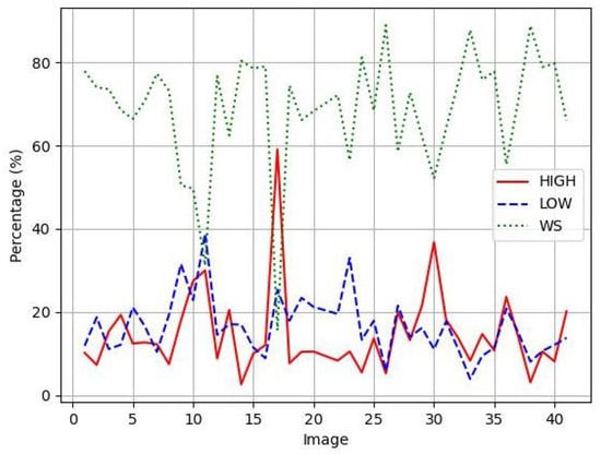
Figure 1.
Percentage of cells for each staining level for all IHC images in OIADB dataset: Nuclei highly stained in red, nuclei low-stained in blue, and nuclei without staining in green.
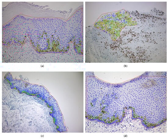
Figure 2.
Examples of original IHC images of OIADB dataset with the expert analysis overlapped: image4 (a), image17 (b), image12 (c), and image34 (d). The region of analysis is drawn in red and the cell’s nuclei as circles in yellow for highly stained nuclei, green for low-stained nuclei, and blue for nuclei without staining.
3. Methods
Image segmentation is often the first essential and critical step in achieving quality outcomes in image analysis systems. The results of a segmentation process are normally represented (1) by a set of connected pixels to define a region or object, being visualized as binary or labeled images; (2) by a set of connected and sorted pixels to define the outline of objects or boundaries; or (3) as lines, corners, or keypoints.
Although segmentation results can be provided by regions or edge segments, both representations are equivalent because it is easy to construct a region from its contour and obtain the contour of an existing region. From the supervision point of view, segmentation techniques can be classified into unsupervised and supervised. There are also proposals to integrate classical unsupervised segmentation techniques into DL approaches [13,14]. These approaches are detailed in the following subsections.
3.1. Unsupervised Image Segmentation
These approaches can be categorized into edge-based, region-based, and hybrid strategies [10]. Region-based segmentation involves partitioning an image into homogeneous areas of connected pixels by applying homogeneity or similarity criteria among the image pixels. Pixels are considered similar on the basis of certain computed properties, such as color, intensity, and/or texture, among others. These techniques assume that the partitions formed represent regions, objects, or meaningful parts of the image. Commonly used techniques include thresholding, region growth, and clustering. Thresholding is the simplest and fastest technique, in which the image is partitioned into sets of pixels with values lower than or higher than a specified threshold [11]. Also, it can be applied locally or globally, but it often yields unsatisfactory segmentations in images with complex backgrounds. Although different methods to calculate the optimal threshold have been proposed in the literature [15], the most popular is the method proposed by Otsu [16]. The region growth methods group pixels or subregions into larger regions based on predefined growth criteria [17]. Among other drawbacks, these methods can be very time-consuming when segmenting large images.
Clustering methods also divide an image into homogeneous regions based on some image property, such as gray level, color, texture, or another [18]. The K-means algorithm is the most popular method due to its simplicity and its very low execution time [10]. Each pixel in the image is considered a pattern, and the K-means algorithm subdivides these patterns into K components by calculating the average patterns for each component. Its main drawbacks are its sensitivity to noise in images and the fact that the selection of the K value affects the quality of the segmentation. The use of image pre-processing techniques may reduce image noise and improve segmentation results. Different improvements on the original algorithm have been addressed in the literature [19]. For example, the MeanShift algorithm [20] does not require the number of clusters as input and calculates this value indirectly using a parameter called the kernel bandwidth.
An edge is considered the boundary of the object, which is manifested as a change or discontinuity in a number of pixels along a certain direction. Edge-based segmentation involves identifying the locations of pixels that correspond to the boundaries of objects present in the image. First and second derivatives are normally used to determine the edge position, marking the pixel as white if it belongs to the boundary of an object and black otherwise. Many edge detectors are available in the literature. They are very sensitive to the presence of noise in the image and cannot detect edgeless objects. However, they have the advantage of requiring a low computation time for application. Canny filter [21] is the most popular due to its trade-off between edge detection and noise attenuation. Edge detectors find the position of pixels in the boundaries of objects, but these pixels must be linked into closed chains of pixels to identify the objects.
The watershed transform is a segmentation method that interprets a grayscale image as a topographical relief, where each pixel is associated with an altitude that corresponds to its intensity. Thus, the pixel values are equivalent to the surface heights defined on a lattice. The main idea is that, as rainwater naturally flows down the steepest paths, the watershed algorithm will eventually fall into a number of domains of attraction. The watersheds are the dividing lines of these domains, called catchment basins, which are the natural segmenting contours of the landscape. The watershed transform is applied to the gradient image to achieve image segmentation. Various algorithms have been proposed to compute the watershed based on different principles. Some popular approaches are the immersion approach and toboggan simulation [22].
Active contour-based models, also called snakes, have long been a popular group. They transform the image segmentation problem into an energy minimization problem, where the energy function specifies the segmentation criterion, and the unknown variables describe the contours of different regions [23]. These methods can be divided into parametric and geometric snakes, depending on whether their representation is explicit using parametric curves or implicit using level-set algorithms [24]. Snakes are considered edge-based models when the parameterized curve of the snake evolves until it reaches high-gradient areas or edges. Since edge-based approaches use gradient functions to stop the evolution of the curve, they struggle with identifying weak edges or edges in noisy images or capturing regions separated by textures. In contrast, geometric snakes are considered region-based models as they employ homogeneity properties to decompose the image domain into different regions, thereby overcoming the aforementioned drawbacks of edge-based approaches. Many of these methods require an initial curve, and its placement on the image plays an important role in the final segmentation, which is a drawback for their application to our problem. The Chan–Vese model is the most representative model, as it can be applied as a region-based and edge-based technique [23].
Image segmentation can also be tackled using graph cuts models, in which the image pixels are the nodes of a weighted graph, and the segmentation problem is translated into finding minimum cut in the constructed velocity graph via a maximum flow computation. Several graph-based methods have been proposed for unsupervised segmentation, including ratio cut [25], normalized cuts [26], and minimum spanning tree-based methods like the efficient Felzenszwalb–Huttenlocher segmentation algorithm [27].
Some recent hybrid segmentation approaches combine different unsupervised segmentation methods typically belonging to various families of algorithms. For example, there are combinations of clustering and watershed to segment white blood cells from microscopy images [28], as well as the integration of region-growing and watershed for cell segmentation in fluorescence microscopy images [29], among others. However, such a combination may increase segmentation accuracy but will likely consume more time.
Taking into account the large size of IHC images and the availability of public code, in this paper we compare the following image segmentation methods:
- OIA-RDA: OralImmunoAnalyser-Region Detection Algorithm is the region-based approach included in the OralImmunoAnalyser (OIA) software to detect nuclei. It combines the K-means clustering algorithm, thresholding by the multi-level Otsu method, and other image pre-processing and post-processing techniques (details in [7]). OIA-RDA has three operation modes, marked by HIGH, LOW, and WS in the OIA graphical interface. The only parameter needed by the algorithm is the minimum diameter of the cells to detect, which is established by the expert pathologists in 20 pixels for the OIDB dataset.
- OIA-EDA: The Multi-Scale Canny Filter (MSCF) is an edge-based method derived from the Canny filter [30]. It applies the Canny filter at different scales, i.e., using various values of Gaussian spread () and different values of hysteresis thresholds, followed by an edge-linking step to produce closed contours. MSCF was configured to be included in OIA with one scale () and one pair of thresholds, with the rates 0.3 and 0.7 for the low and high thresholds, respectively, denominated as OIA-EDA in this paper. The minimum diameter of the cells to detect is also set to 20 pixels for the OIDB dataset.
- FH: The Felzenszwalb–Huttenlocher algorithm [27] is selected among the graph cut models due to its efficiency and the availability of an implementation in the segmentation module of the Python scikit-image library (https://scikit-image.org/). We use the Felzenszwalb function, configured with default values (scale = 1.0 and sigma = 0.8), except for the minimum component size , which is set to 400 pixels. Since the minimum diameter of the cells provided by the experts is 20 pixels for the OIADB dataset, we assume the minimum size of the components are a square of the minimum size diameter, .
- ChV: Among the active contour models, we select the Chan–Vase algorithm [23], implemented also in the Python scikit-image library and which does not need to provide initial seeds to its application. Specifically, we use the morphological_chan_vese function to apply Morphological Active Contours without Edges, called MorphACWE, and the Morphological_geodesic_active_contour function to apply Morphological Geodesic Active Contours, called MorphGAC. Both methods are applied using default configurations (using 500 iteractions), and the original images were pre-processed with a Gaussian filter of size ( pixels) to reduce noise in the images.
- Clustering: The available clustering algorithms used are (1) the popular K-means algorithm implemented by the kmeans function in the OpenCV library (https://opencv.org/) using the original image in the RGB and Lab color spaces, designed as kmeans-RGB and kmeans-LAB, respectively; and (2) the slic function of the segmentation API of the scikit-image library, which implements the simple linear iterative clustering (SLIC) superpixels method [31], called SLIC. In the kmeans-RGB approach, the kmeans function is applied on patterns including the RGB signature of each pixel in the image using four clusters (one for each staining level of nuclei and another for the sample background). Initial centers for the clusters are taken randomly, and we use the default configuration for the remaining parameters (the algorithm stops when 10 iterations of the algorithm have run or an accuracy of epsilon = 1.0 is reached). A signature containing the three values of the channels of the Lab color space is used for the kmeans-LAB approach.
Although there is available code to implement the watershed algorithm in the OpenCV library, we rejected its application to our problem because it is an iterative algorithm that requires placing markers on the local minima in the image to set the starting points, which must correspond precisely to the nuclei positions.
We would like to emphasized that these five unsupervised methods use the same values for each parameter in all the images (these values are the default ones for each method), including the minimum diameter of the cells to detect, which is set by experts as commented above. Therefore, these methods are completely unsupervised, because their parameters are set without using the dataset in any way.
3.2. Supervised Image Segmentation Using Deep Learning
In the last two decades, supervised image segmentation and object detection have been developed predominantly using deep learning (DL). Among the DL techniques proposed in the literature [32], the different variants of the U-Net and YOLO (You Only Look Once) architectures are the most prominent for image segmentation and object detection [33,34].
3.2.1. U-Net
Cell segmentation and detection on histopathology [35] or RGB immunofluorescence [36] images are commonly performed using the U-Net deep neural network [34] and its variants. U-Net consists of two primary components: an encoder and a decoder. The encoder processes the input image, gradually reducing its spatial dimensions while extracting higher-level features, effectively compressing the image into a lower-dimensional representation. The decoder then reconstructs the image from this compressed representation, upsampling it to produce the final output, which varies depending on the task. For example, in semantic segmentation, the input is an image, and the output is a segmentation mask that highlights the regions of interest [34]. Figure 3 illustrates the typical diagram of the U-Net architecture.
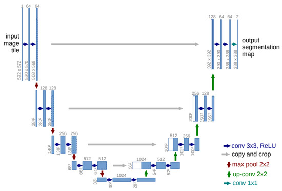
Figure 3.
Typical diagram of U-Net architecture.
U-Net allows the selection of a specific encoder from a wide range of convolutional neural networks (CNN) available in the timm library [37], a popular repository that provides access to numerous CNN architectures pre-trained on large-scale datasets such as ImageNet. In our case, we use the segmentation-models-pytorch (SMP) module (https://pypi.org/project/segmentation-models-pytorch/0.0.3/, accessed on 10 September 2025) with the pre-trained EfficientNet-B0 model as the encoder for our U-Net architecture. EfficientNet-B0 is known for its strong performance-to-parameter ratio, enabling efficient feature extraction with relatively low computational cost. Using pre-trained weights, the model benefits from transfer learning, which accelerates convergence and improves performance, especially in scenarios with limited labeled data.
Like most deep learning architectures, U-Net requires a substantial amount of training data to perform effectively. To mitigate data scarcity in our methodology, we divide each image into non-overlapping patches of size pixels (model input size). This process increases the number of training samples to approximately 2000. These patches serve as input to the proposed U-Net model. The corresponding outputs, called targets, are heatmaps in which the cell locations are encoded using 2D Gaussian functions ( and peak 5) centered on the ground-truth cell centroids. This heatmap representation enables the model to learn the spatial location of cells without relying on explicit segmentation. The U-Net model is trained using AdamW (weight decay = ).
To further enrich the dataset and reduce the risk of overfitting, we apply image augmentation techniques [38]. These techniques introduce slight variations to the input patches before feeding them into U-Net, ensuring that it does not see the exact same images across training epochs. This strategy is a well-established practice in training deep learning models and helps improve generalization performance. In this work, the applied augmentations include color jittering (adjusting brightness, contrast, saturation, and hue), horizontal and vertical flipping, Gaussian blurring with a kernel size of 5 and a variable sigma range (0.01 to 2), and the addition of Gaussian noise with a standard deviation sampled from the range 0.01 to 0.2. These transformations are applied using the torchvision transforms and are composed as part of the training data pipeline. Figure 4 shows an example of a single input patch with its corresponding heatmap.
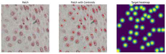
Figure 4.
Original image patch (left panel); ground-truth centroids overlapped to the image in red (middle panel); and the corresponding target heatmap (right panel).
Both input patches and output targets are normalized to the range (0–1) to ensure numerical stability during training and to facilitate faster model convergence [39]. In particular, normalizing the target heatmaps is essential for stable loss computation and contributes to more effective optimization by keeping the target values within a consistent and predictable scale.
To effectively train the U-Net network for accurate point detection using heatmap regression, we define the following composite loss function, , that integrates a weighted Binary Cross-Entropy (BCE) loss with a spatially weighted Mean Squared Error (MSE) loss:
where denotes the predicted logit at pixel i, is the corresponding ground-truth heatmap value, represents the sigmoid activation applied to the logit at pixel i, N is the total number of pixels in the heatmap, and are weighting coefficients for the BCE and weighted MSE loss components respectively, and is the spatial weighting parameter. The coefficients were empirically chosen as and to balance classification and localization performance. The BCE loss operates directly on logits and incorporates positive class weighting to mitigate class imbalance between sparse foreground peaks and the dominant background. The weighted MSE component applies spatial weighting where each pixel is weighted by with , increasing loss contribution from regions with higher target values to encourage sharper, more localized heatmap peaks centered on annotated points.
This parameter determines the contribution of the weighted MSE component. A higher value (0.7) emphasizes spatial accuracy, encouraging the model to produce precise and smooth heatmaps that match the ground-truth intensity distribution around annotated points. The value controls the degree of spatial weighting in the MSE loss. The term increases the importance of pixels with higher target values (typically near keypoint centers). A value of 10 strongly emphasizes these areas, helping the model focus on accurately localizing keypoints while reducing the influence of distant background pixels.
Despite the logical selection of the coefficients , and , we acknowledge that these hyperparameters were not systematically optimized and should be systematically optimized in future applications of this loss function to potentially achieve better performance.
After training the model, a test image is passed as a set of patches to obtain the predicted heatmap. Figure 5 shows visual examples of the performance of the U-Net model. To locate the centroids, the predicted heatmaps are first smoothed using a Gaussian filter to suppress spurious local maxima. Then, a maximum filter is applied to identify peaks in the heatmap. Only peaks with values above a predefined threshold (default: 0.5) are retained. To address multiple detections for the same cell, we remove redundant peaks that fall within a specified perimeter (20 pixels, which is the minimum diameter of the cells in the OIADB dataset). When multiple peaks are found within this perimeter, their mean position is taken as the final centroid.
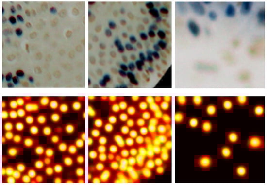
Figure 5.
The first row has samples from the test set, and the second row shows their corresponding predicted heatmaps.
3.2.2. YOLO
Another neural network widely used for object detection is YOLO, renowned for its high speed and efficiency in detecting objects and predicting their corresponding bounding boxes. Its ability to perform detection in real time makes it particularly suitable for various time-sensitive applications [32,33]. In the current work, we employ YOLOv8 (nano variant), the latest version of the YOLO architecture, implemented using the Ultralytics library (https://github.com/ultralytics, accessed on 10 September 2025) (version 8.3.0). The input images are divided into patches following the same strategy described in Section 3.2.1 for the U-Net model. In YOLO, the Ultralytics library handles image normalization internally, automatically scaling pixel values to the range (0–1) during both training and inference phases. Also, it uses internal augmentation techniques to enrich the training dataset.
Unlike U-Net, YOLO does not predict heatmaps, but bounding boxes. Since our dataset does not include bounding-box annotations, but only the coordinates of cell centroids, we generate synthetic bounding boxes by centering a fixed-size square around each centroid. Specifically, each bounding box extends 5 pixels equally in all directions from the centroid, resulting in a region of pixels per cell. While this is smaller than the minimum cell diameter of 20 pixels, this approach is justified because (1) our task focuses on centroid localization rather than full cell detection; (2) YOLOv8 employs an anchor-free architecture with automatic anchor assignment, eliminating anchor box mismatch issues; (3) YOLO’s convolutional layers process contextual information through their receptive fields, allowing access to full cell information beyond bounding box boundaries; and (4) smaller boxes reduce computational overhead and minimize overlap between adjacent cells.
The YOLOv8 model was initialized with pre-trained weights from the COCO dataset (transfer learning) and trained using its default composite loss, which combines classification, IoU-based bounding box regression, and objectness terms. During training, the same augmentations applied to U-Net were used, including flipping, color jittering, Gaussian blurring, and noise addition. Optimization was performed using the default optimizer, Stochastic Gradient Decent (SGD with momentum = 0.937), with a cosine annealing learning rate schedule, starting at and decaying to over 50 epochs.
YOLO typically makes classifications of the detected objects. However, in this work, we are concerned with the detection of cells without making a classification of the cell staining level. In this way, we make its results comparable to the remaining segmentation methods.
It is worth mentioning here that no morphological filtering is done to any feature map in any of the used DL models, including the output feature map of U-Net.
4. Results
The methods described in Section 3.1 and Section 3.2 for cell detection are applied to the IHC images introduced in Section 2. The following sections present the metrics used to evaluate the performance (Section 4.1), the experimental setup (Section 4.2), and the quantitative results achieved by unsupervised (Section 4.3) and supervised (Section 4.4) techniques. Subsequently, Section 4.5 reports the computation time, and Section 4.6 discusses the results.
4.1. Metrics of Detection Performance
Statistical evaluation is crucial for assessing and comparing the detection methods used. The choice of metrics depends on both the segmentation output format and the nature of the ground-truth data. Segmentation techniques may produce boundary-based outputs (e.g., pixel-wise contours), region-based results (e.g., segmented objects), or keypoint-based representations (e.g., sparse feature points), each requiring different evaluation approaches. Ground-truth data further influence metric selection, as well-posed problems with a single definitive solution allow for direct comparison, while poorly posed problems, where multiple valid interpretations exist, demand more flexible evaluation strategies.
Regarding the cell detection on immunohistochemistry (IHC) images, ground-truth annotations are typically provided as scribbles, bounding boxes, or points marking the x and y coordinates of cells. Given the nature of this problem, we adopt an indirect evaluation framework tailored to cell detection by treating segmentation performance as a detection task and using the -score for statistical assessment. Here, true positives (TP ) represent correctly detected cells, false positives (FP) denote erroneously detected non-cells, and false negatives (FN) correspond to missed true cells. In this study, the evaluation metrics, recall (R), precision (P), and -score () are defined as follows:
To evaluate cell detection performance, we compare the positions of segmented nuclei against ground-truth cell positions. A segmented nucleus is counted as a true positive (hit) if its position lies within the minimum diameter of a true cell nucleus; otherwise, it is considered a false negative (miss). When multiple true cells satisfy this distance criterion for a single segmented nucleus, it is counted only once to avoid overestimation. Any segmented nucleus that does not meet this proximity requirement with any true cell is classified as a false positive. This rigorous matching approach ensures accurate quantification of detection performance in our analysis.
In order to study the performance of segmentation algorithms in relation to the level of nuclei staining in IHC images, we calculate the accuracy of hits for each type of nuclei for an image as
where is the accuracy (%) for detecting nuclei with staining level X, is the number of correctly detected nuclei with staining level X, and is the total number of nuclei with staining level X in the image.
4.2. Experimental Setup
The experiments in this study are designed to fit the two used approaches: supervised and unsupervised segmentation. In the unsupervised segmentation, the algorithms described in Section 3.1 are applied to the IHC images in order to calculate the position of detected cells. When the output of the method is a labeled or binary image (in the case of FH, ChV, and clustering methods), we applied the following post-processing step. Let and be the minimum and maximum area of a true cell calculated as the area of a circle with the minimum and maximum diameters of the cells established by pathologists for this dataset. The regions in the segmented image whose areas fall within the interval [, ] are considered candidates to represent true cells, whose positions will be the mass center of those regions. In the supervised DL approach, we employ a leave-one-IHC-image-out (LOO) cross-validation approach, which is particularly suitable given the limited size of the OIADB dataset. This methodology ensures a fair evaluation by iteratively selecting all patches of each IHC image in the dataset as the test sample, while the patches of the remaining images are used to train the model. This methodology ensures that all images in the dataset are used to test the method, as in the case of unsupervised algorithms. According to this methodology, it is not possible that patches of the same image are present in both the training and test sets. Therefore, there is no data leakage nor inflated performance estimates (i.e., optimistic bias). Since each image corresponds to a different patient, i.e., each patient has only one image, it is not possible that information about the same patient is used both in the training and test datasets.
Both models, U-Net and YOLO, are trained for 50 epochs, with early stopping (patience = 5), to strike an optimal balance between underfitting and overfitting, allowing the model sufficient time to learn the underlying patterns without an excessive risk of overfitting. The training batch size is set to 16, balancing computational efficiency with graphical processing unit (GPU) memory constraints to enable smoother training. The models are trained using a learning rate schedule, which starts at 0.01 and follows a cosine annealing pattern that decays to 0.001 during the course of training. This scheduling strategy automatically adapts well to our patch-based training approach. Stochastic gradient descent is used as an optimizer, with a momentum of 0.937 and weight decay set to 0.0005.
Finally, for all the methods, an overlapping test is applied in order to avoid two detections of the same true cell. If the distance between the position of two cells is smaller than the minimum diameter, we assume that these two positions correspond to the same true cell.
4.3. Cell Detection Using Unsupervised Segmentation
Table 1 shows the average precision, recall, and -score for all the unsupervised segmentation techniques used in this study. OIA-RDA provides a high precision, about 87.6%. Recall and -score increase from option HIGH (R = 8.4% and = 15%) to option WS (R = 24.4% and = 35.9%), but recall is low for all configurations, although the performance depends on the specific image. OIA-RDA achieves good performance for the detection of highly stained cells, detecting 63.9% of the highly stained cells, but its reliability is poor for detecting the low-stained or nonstained cells, where it detects less than 24% and 15.8% of low-stained and nonstained cells, respectively. A behavior similar to OIA-RDA, although with lower global performance, is observed by active contour approaches (ChV) with an average = 21% (P = 89.4%, R = 12.6%). On the other hand, OIA-EDA shows a performance more balanced (i.e., R and P more similar between them) than OIA-RDA, achieving R = 44.1% and P = 46.7% with = 41.0%; that is the highest performance over all unsupervised methods. This edge-based segmentation technique exhibits a uniform behavior with respect to the level of cell staining (see the last three columns of Table 1), but its main drawback is the high number of false positives due to its moderate precision. The FH graph cut method shows similar behavior to OIA-ED, but with lower overall performance: = 34.5% (P = 40.9% and R = 34.6%). Clustering-based approaches generally underperform, with K-means implementations in both the RGB and Lab color spaces yielding recall and precision values around 12–13% and 40%, respectively, and correspondingly low scores (16.7–17%). The SLIC clustering method performs particularly poorly, with near-negligible recall (0.3%) and precision (4.2%). Quantitative results of the MeanShift algorithm are not provided due to its very poor performance.

Table 1.
Precision, recall, and -score (columns three, four, and five) with standard deviation to detect the cell’s nuclei in IHC images of the OIADB dataset. The column p-value refers to a Wilcoxon ranksum test comparing the -score of U-Net and the other methods. The last three columns (, , and ) show the accuracy of (%) detecting high, low, and without-staining levels of nuclei.
From the common behavior of OIA-RDA and OIA-EDA, we can assert thatthe OIA-RDA method provides better results when the IHC images contain higher rates of stained cells (as, for example, image 17 in Figure 2), for which it frequently provides a low number of false positives and all the detected cells are really true cells, giving high precision values. On the other hand, OIA-EDA detects more cells (recall higher than OIA-RDA) and works better for detecting low and nonstained cells due to the fact that they are normally isolated, as in images 4 or 12 in Figure 2. Since both algorithms are available in the OralImmunoAnalyser (OIA) software for experts to run separately or in combination, we experimented by adding the cells detected by both approaches (see the row with Method = OIA and Config = RDA-EDA in Table 1). The performance metrics increased slightly to R = 49.2%, P = 50.9%, and = 46.4%, and OIA-RDA-EDA emerges as the most effective unsupervised segmentation method.
4.4. Cell Detection Using Deep Learning
The deep learning networks U-Net and YOLO, described in Section 3.2, are applied to the segmentation of IHC images of the OIADB dataset employing the leave-one-image-out cross-validation configuration described in Section 4.2. Average precision, recall, and -score values are computed for a collection of values for the parameters threshold and diameter. The threshold (called confidence in the YOLO model) controls the heatmap intensity level at which centroids are captured, and the diameter defines the allowable distance between a predicted cell position and a ground-truth point for the prediction to be considered correct. Threshold values ranging from 0.1 to 0.9 with step 0.1 are considered. The diameter values are established, taking into account the minimum diameter of cells in this dataset, which is 20 pixels. So, we use diameter values close to 20, ranging from 10 to 30 with step 1.
Figure 6 shows the heatmaps with the average precision, recall, and -score for all IHC images under different threshold and diameter values for the U-Net model (upper row) and YOLO model (lower row). The performance value is overlapped on the heatmap as a number (in percentage) and also coded as a different color. U-Net slightly outperforms YOLO, achieving the highest -score, approximately 77%, for thresholds in the range of 0.4 to 0.7 and diameters between 10 and 13 pixels. Precision reaches its maximum values at higher thresholds (0.8–0.9) within the same diameter range, indicating a reduction in false positives. In contrast, recall is the highest at lower thresholds (0.1–0.2), reflecting increased sensitivity to true positives under more permissive detection criteria. In this study, we focused on the parameter combinations that maximize the -score as it provides a balanced trade-off between precision and recall. Specifically, we selected the operation point on a threshold of 0.6 and a diameter of 11 pixels. For the YOLO model, we selected the operation point of threshold = 0.1 and diameter = 14 pixels.
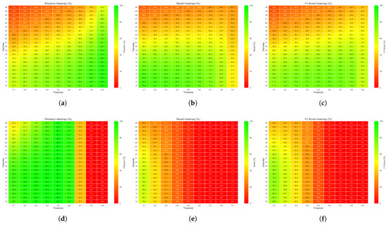
Figure 6.
Average precision: (a) for U-Net and (d) for YOLO; recall: (b) for U-Net and (e) for YOLO; and -score: (c) for U-Net and (f) for YOLO, across the images in the dataset, using different threshold (x-axis) and diameter (y-axis) values.
The last two rows of Table 1 show the performance for the deep learning models. U-Net achieves the highest performance with = 75.3%, R = 74.4%, and P = 76.8%. A low precision indicates a high rate of false positives, which may lead to incorrect detections, while a low recall suggests that many true positives are missed, reducing the sensitivity of the model. YOLO is slightly lower, in terms of , achieving = 74.0%, R = 69%, and P = 81%. Both deep learning networks show consistent behavior depending on the level of cell staining, as seen in the last three columns of Table 1 (accuracy ranging from 63% to 77% for both DL models and all staining levels of the cell’s nuclei). Figure 7 shows some patches, extracted from the test set, with their true and predicted centroids for the two DL models. After collecting the predicted centroids from the individual patches of a test image, we map these centroids to the original image. Figure 8 and Figure 9 illustrate the final prediction result on image34 and image12, respectively, of the OIADB dataset using the best performing methods in this study: the unsupervised segmentation algorithms included in OralImmunoAnalyser software (the region-based approach, OIA-RDA; the edge-based approach, OIA-EDA; and a combination of both, OIA-RDA-EDA) and the deep learning approaches U-Net and YOLO. For image 34, the -score is 64.5% for OIA-RDA, 46.8% for OIA-EDA, 52.2% for OIA-RDA-EDA, 87.5% for U-Net, and 86.6% for YOLO. For image 12, the -score is 22.6% for OIA-RDA, 42.4% for OIA-EDA, 46.5% for OIA-RDA-EDA, 72.1% for U-Net, and 70.9% for YOLO.
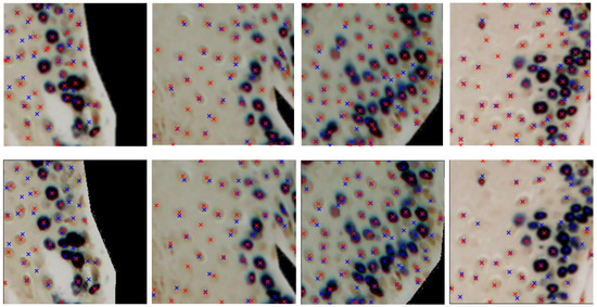
Figure 7.
Samples from the dataset with the ground-truth and the predicted centroids, using U-Net (top panel) and YOLO (bottom panel), highlighted as blue and red crosses, respectively.
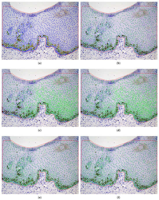
Figure 8.
Example (image34) of cell detection (cells are overlapped to the IHC image) for unsupervised segmentation approaches: (b) OIA-RDA (option WS); (c) OIA-EDA; (d) OIA-RDA-EDA; (e) U-Net; and (f) YOLO. The ground truth of image 34 is the upper left panel (a), where the color means the staining level of nuclei: yellow (highly stained), green (low-stained), and blue (without staining).
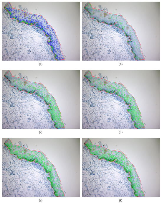
Figure 9.
Example (image 12) of cell detection of unsupervised segmentation approaches (cells are overlapped to the IHC image) for the different approaches: (b) OIA-RDA (option WS); (c) OIA-EDA; (d) OIA-RDA-EDA; (e) U-Net model; and (f) YOLO model. Panel (a) shows the ground truth, where the color means the staining level of nuclei: yellow (highly stained), green (low-stained), and blue (without staining).
4.5. Computation Time
The unsupervised segmentation experiments were performed on a desktop computer with an Intel® CoreTM i7-9700 processor at 3.6 GHz and 64 GB of RAM under Ubuntu 24.04. The OIA algorithms were done in the C/C++ programming language using the OpenCV 4.6 computer vision library, and the remaining algorithms were implemented in the Python 3.12.3 and scikit-image 0.22 libraries.
The deep learning experiments were conducted on a Windows Server 2022 Standard Evaluation 64-bit (10.0, Build 20348) with Intel(R) Xeon(R) Gold 6426Y (64 CPUs), ∼2.5 GHz with 128 GB of RAM memory, equipped by a GPU NVIDIA RTX A4000 with 8 GB of RAM memory. All deep learning experiments were implemented using Python programming language. U-Net was imported from the segmentation-models-pytorch (SMP) module (https://pypi.org/project/segmentation-models-pytorch/0.0.3/, accessed on 10 September 2025). The preparation of datasets and data load was performed using PyTorch (2.7.0.dev20250122+cu126). For YOLO, we used the implementation provided by Ultralytics (https://github.com/ultralytics, accessed on 10 September 2025).
The average computational time per image for each method is shown in Table 2. For unsupervised segmentation methods, the computational time also includes the pre- and post-processing steps. The algorithms included in OralImmunoAnalyser are the fastest, requiring only approximately one second to process an image, making them optimal for interactive applications. The slowest algorithms are the active contours, which take nearly 10 min to process a single image. The methods based on clustering or graph cuts fall in between, with processing times ranging from a few seconds for K-means approaches to up to two minutes for the FH graph cut method. The last four rows of Table 2, named U-Net and YOLO, report the average times spent by these networks to process a image, i.e., the average time spent to test the deep network on one image. The rows labeled with “using CPU” indicate the computational time needed by the DL technique to process a test image without employing specialized hardware, i.e a GPU. These test times, which do not include the time required to train the DL network, are similar to the fastest unsupervised segmentation methods. Training deep neural networks is very intensive, even using dedicated hardware like GPUs. In our case, it takes approximately between 4 to 6 h.
Table 2.
Computational time of segmentation approaches.
4.6. Discussion
Regarding the cell detection performance in Table 1, the best = 75.3% is provided by a supervised technique, the U-Net deep learning model. The best unsupervised segmentation technique, OIA-RDA-EDA, included in the OralImmunoAnalyser software [7], achieved = 46.4%. Figure 10 shows the average precision (blue bars), recall (green bars), and -score (red bars) for the best supervised and unsupervised approaches tested on the OIADB dataset. The vertical error bars show the standard deviation of each method. As expected, supervised techniques provided the highest performance results, because they use knowledge of the problem (location of the cell’s nuclei) through training before processing a test image. Figure 11 shows the precision, recall, and -score achieved by the best method for both approaches to detect cells in IHC images for each image in the OIADB dataset. Table 1 also includes a column reporting the p-value of a Wilcoxon ranksum test comparing the -score of U-Net and of the other methods. This difference is not statistically significant only for YOLO (p-value = 0.358122), being significant for the others with , marked in Table 1 as . This means that both deep learning methods, U-Net and YOLO, clearly outperform the unsupervised methods.
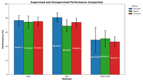
Figure 10.
Average of precision, recall, and -score for the best supervised and unsupervised segmentation algorithms tested on OIADB dataset.
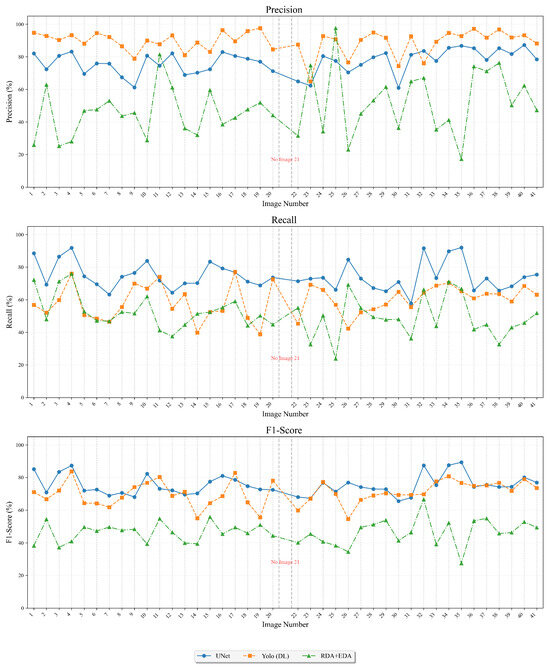
Figure 11.
Precision (upper panel), recall (middle panel), and -score (lower panel) for each image in the dataset for the U-Net model (blue line), OIA-EDA (orange line), and RDA + EDA (green line).
There are a number of difficulties when comparing the computational resources needed for supervised versus unsupervised segmentation approaches. Traditional segmentation methods such as edge detection, thresholding, and clustering are often made to function well on common hardware. Generally speaking, these techniques can be used on a general-purpose computer and often finish processing in a respectable amount of time, approximately one or two seconds for average images. Because of this, users with little processing power can utilize them.
However, supervised segmentation methods, especially those that rely on deep learning, require much more processing power. Due to the large number of calculations required for training and inference, these methods often require specialized hardware, such as graphics processing units (GPUs) or tensor processing units (TPUs). Many layers and parameters are commonly included in deep learning models used for segmentation/detection, which can result in increased memory needs and processing times. Consequently, the application of these techniques can be limited to settings with high-performance computer capability. One important point to mention here is the fact that DL inference (or test) time is very low compared to its training time; see Table 2. Another drawback for the practical use of deep learning is that the training stage needs a collection of annotated images. This requirement does not exist for the unsupervised methods, which process each image independently and do not need any collection that may be difficult or impossible to gather or to annotate.
Furthermore, the deep learning models’ training phase may be especially resource-intensive, frequently needing huge datasets and a significant amount of time to reach peak performance. This stands in stark contrast to conventional approaches, which may often be used immediately without requiring large datasets or intensive training. Overall, even though deep learning methods can produce better detection outcomes, especially in complex situations, their increased resource consumption and dependence on specialized hardware may make them impractical for some applications, particularly in settings with limited computational resources. Since deep learning models can be run on general-purpose (CPU-only) computers in a reasonable amount of time, the technological limitations for small biomedical units could be overcome if they have facilities for computing-intensive structures to train deep learning algorithms.
Note that the use of ground truth by deep learning methods (U-Net and YOLO) does not mean that comparison to unsupervised method is unfair. Rather, this is a fundamental difference between both methodological approaches. Their comparison is of practical relevance because it highlights research between investing time in data annotation and supervised training or applying readily available unsupervised methods, reporting the trade-off between these two legitimate strategies for cell detection. The conclusions of our study are that supervised methods achieve superior performance, but at the cost of requiring training data and computational resources.
Recently, the study [1] tested the performance of deep learning-based digital image analysis systems relative to manual counting by expert pathologists in stomach cancer tissues using IHC images stained with the ki-67 biomarker. The study compared three systems (AetherAI, 3D Histech, Roche), analyzing 239 microscopic specimens, and found considerable variability among the results. No deep learning-based application exceeded the average performance among human experts, and variability also occurred among the experts themselves, according to the method of counting (whole TMA, box selection, or hand-free selection). These results indicate the potential, but also the current shortcomings, of deep learning systems in this field, evidencing the need for further research.
5. Conclusions and Future Work
In this study, we presented a comprehensive evaluation of cell detection methods applied to immunohistochemical (IHC) images of oral tissue, comparing traditional unsupervised segmentation techniques with modern deep learning-based approaches. The results demonstrated that classical methods such as K-means clustering, edge detection, and active contours can provide acceptable performance under specific conditions. For example, highly stained cells are well-detected by the region-based algorithm OIA-RDA. Although they are very fast (needing only one or two seconds per image) and do not require specific hardware resources, they are generally limited in handling the complexity of some IHC images, particularly in the presence of artifacts or defects in sample preparation. Globally, the highest performance achieved is only = 46.4% using OIA-RDA-EDA. Regarding their performance in detecting cells with different levels of staining, region-based techniques such as OIA-RDA were highly sensitive in detecting highly stained cells (63.9% of highly stained cells) and achieved low sensitivity with the rest of the staining levels. However, recent research suggests that intensely stained cells are associated with specific cellular phases, being present more often in cases of invasive carcinoma or carcinoma in situ. This makes their detection particularly important. On the other hand, unstained or lightly stained cells identify cellular phases that may be consistent with normality or the presence of hyperplasia. Edge-based algorithms, such as OIA-EDA, perform uniformly with all levels of cell staining.
As expected, the supervised cell detection using deep learning models achieved better performance than unsupervised segmentation, because they used the problem knowledge during the training step before their use for cell detection. The U-Net network, employing heatmap regression to detect cell centroids, achieved the highest performance, = 75.3%. YOLOv8, adapted with synthetic bounding boxes, also showed strong results, = 74%. As well, the behavior of both methods was uniform with all staining levels of cells. This highlights the effectiveness of deep learning for robust and scalable cell detection in histopathological analysis.
Despite the promising results, the study acknowledges the limitations posed by the relatively small number of IHC images in the OIADB dataset and the reliance on centroid-only annotations, but cell drawing labeling requires a great deal of workload for professionals. However, we want to highlight that each image has on average more than 1000 cells, so the dataset has more than 40,000 labeled cells, which is a significant number of objects to detect. Despite all this, the generalizability of the results could be further improved by including a comprehensive comparative study evaluating our methods against other published cell detection approaches across larger standardized datasets to provide broader performance benchmarking. Additionally, we plan to extend our evaluation to include cross-dataset generalization studies to assess method robustness across different tissue types and imaging protocols.
Future work will aim to extend the deep learning models YOLO and U-Net to also make classifications of the cell staining levels of the detected objects. We are also planning to include a trained deep learning U-Net model in the OralImmunoAnalyser software.
Author Contributions
Conceptualization, Z.A.A.-T., A.S.T., P.G.-V. and E.C.; methodology, Z.A.A.-T., A.S.T., A.M., M.F.-D. and E.C.; software, Z.A.A.-T., A.S.T., A.M. and E.C.; validation, Z.A.A.-T. and E.C.; formal analysis, Z.A.A.-T., A.S.T. and E.C.; investigation, Z.A.A.-T., A.S.T., A.M. and E.C.; resources, M.F.-D. and E.C.; data curation, Z.A.A.-T. and A.M.; writing—original draft preparation, Z.A.A.-T. and E.C.; writing—review and editing, all authors; visualization, Z.A.A.-T.; supervision, E.C. and Z.A.A.-T.; project administration, E.C.; funding acquisition, E.C. All authors have read and agreed to the published version of the manuscript.
Funding
This research received no external funding.
Institutional Review Board Statement
Not applicable.
Informed Consent Statement
Not applicable.
Data Availability Statement
OIADB dataset: https://gitlab.citius.gal/analyser/oiadb, accessed on 10 September 2025.
Acknowledgments
This work has received financial support from the Xunta de Galicia—Consellería de Cultura, Educación, Formación Profesional e Universidades (Centro de investigación de Galicia accreditation 2024–2027, ED431G-2023/04) and the European Union (European Regional Development Fund—ERDF).
Conflicts of Interest
The authors declare no conflicts of interest.
Abbreviations
The following abbreviations are used in this manuscript:
| GPU | Graphics Processing Unit |
| RAM | Random Access Memory |
| CPU | Central Processing Unit |
| GB | Gigabyte |
| DL | Deep Learning |
References
- Alam, M.R.; Seo, K.J.; Yim, K.; Liang, P.; Yeh, J.; Chang, C.; Chong, Y. Comparative analysis of Ki-67 labeling index morphometry using deep learning, conventional image analysis, and manual counting. Transl. Oncol. 2025, 51, 102159. [Google Scholar] [CrossRef]
- Azevedo Tosta, T.A.; Neves, L.A.; do Nascimento, M.Z. Segmentation methods of H&E-stained histological images of lymphoma: A review. Inform. Med. Unlocked 2017, 9, 35–43. [Google Scholar] [CrossRef]
- Sand, F.L.; Lindquist, S.; Aalborg, G.L.; Kjaer, S.K. The prognostic value of p53 and Ki-67 expression status in penile cancer: A systematic review and meta-analysis. Pathology 2025, 57, 276–284. [Google Scholar] [CrossRef] [PubMed]
- Rodríguez-Candela Mateos, M.; Azmat, M.; Santiago-Freijanes, P.; Galán-Moya, E.M.; Fernández-Delgado, M.; Aponte, R.B.; Mosquera, J.; Acea, B.; Cernadas, E.; Mayán, M.D. Software BreastAnalyser for the semi-automatic analysis of breast cancer immunohistochemical images. Sci. Rep. 2024, 14, 2995. [Google Scholar] [CrossRef]
- Torres, L.A.F.; Celso, D.S.G.; Defante, M.L.; Alzogaray, V.; Bearse, M.; de Melo Lopes, A.C.F.M. Ki-67 as a marker for differentiating borderline and benign phyllodes tumors of the breast: A meta-analysis and systematic review. Ann. Diagn. Pathol. 2025, 75, 152429. [Google Scholar] [CrossRef]
- Dias, E.P.; Oliveira, N.S.C.; Serra-Campos, A.O.; da Silva, A.K.F.; da Silva, L.E.; Cunha, K.S. A novel evaluation method for Ki-67 immunostaining in paraffin-embedded tissues. Virchows Arch. 2021, 479, 121–131. [Google Scholar] [CrossRef]
- Al-Tarawneh, Z.A.; Pena-Cristóbal, M.; Cernadas, E.; Suarez-Peñaranda, J.M.; Fernández-Delgado, M.; Mbaidin, A.; Gallas-Torreira, M.; Gándara-Vila, P. OralImmunoAnalyser: A software tool for immunohistochemical assessment of oral leukoplakia using image segmentation and classification models. Front. Artif. Intell. 2024, 7, 1324410. [Google Scholar] [CrossRef]
- Đokić, S.; Gazić, B.; Grčar Kuzmanov, B.; Blazina, J.; Miceska, S.; Čugura, T.; Grašič Kuhar, C.; Jeruc, J. Clinical and Analytical Validation of Two Methods for Ki-67 Scoring in Formalin Fixed and Paraffin Embedded Tissue Sections of Early Breast Cancer. Cancers 2024, 16, 1405. [Google Scholar] [CrossRef]
- Gupta, A.; Duggal, R.; Gehlot, S.; Gupta, R.; Mangal, A.; Kumar, L.; Thakkar, N.; Satpathy, D. GCTI-SN: Geometry-inspired chemical and tissue invariant stain normalization of microscopic medical images. Med. Image Anal. 2020, 65, 101788. [Google Scholar] [CrossRef]
- Gonzalez, R.; Woods, R. Digital Image Processing Global Edition; Pearson Deutschland: Munich, Germany, 2017; p. 1024. [Google Scholar]
- Brar, K.K.; Goyal, B.; Dogra, A.; Mustafa, M.A.; Majumdar, R.; Alkhayyat, A.; Kukreja, V. Image segmentation review: Theoretical background and recent advances. Inf. Fusion 2025, 114, 102608. [Google Scholar] [CrossRef]
- Minaee, S.; Boykov, Y.; Porikli, F.; Plaza, A.; Kehtarnavaz, N.; Terzopoulos, D. Image Segmentation Using Deep Learning: A Survey. IEEE Trans. Pattern Anal. Mach. Intell. 2022, 44, 3523–3542. [Google Scholar] [CrossRef] [PubMed]
- Xie, L.; Qi, J.; Pan, L.; Wali, S. Integrating deep convolutional neural networks with marker-controlled watershed for overlapping nuclei segmentation in histopathology images. Neurocomputing 2020, 376, 166–179. [Google Scholar] [CrossRef]
- Pina, O.; Vilaplana, V. Unsupervised Domain Adaptation for Multi-Stain Cell Detection in Breast Cancer with Transformers. In Proceedings of the 2024 IEEE/CVF Conference on Computer Vision and Pattern Recognition Workshops (CVPRW), Seattle, WA, USA, 17–18 June 2024; pp. 5066–5074. [Google Scholar] [CrossRef]
- Jardim, S.; António, J.; Mora, C. Image thresholding approaches for medical image segmentation—Short literature review. Procedia Comput. Sci. 2023, 219, 1485–1492. [Google Scholar] [CrossRef]
- Otsu, N. A Threshold Selection Method from Gray-Level Histograms. IEEE Trans. Syst. Man Cybern. 1979, 9, 62–66. [Google Scholar] [CrossRef]
- Fan, J.; Zeng, G.; Body, M.; Hacid, M.S. Seeded region growing: An extensive and comparative study. Pattern Recognit. Lett. 2005, 26, 1139–1156. [Google Scholar] [CrossRef]
- Bayá, A.E.; Larese, M.G.; Namías, R. Clustering stability for automated color image segmentation. Expert Syst. Appl. 2017, 86, 258–273. [Google Scholar] [CrossRef]
- Shao, J.; Chen, S.; Zhou, J.; Zhu, H.; Wang, Z.; Brown, M. Application of U-Net and Optimized Clustering in Medical Image Segmentation: A Review. CMES—Comput. Model. Eng. Sci. 2023, 136, 2173–2219. [Google Scholar] [CrossRef]
- Comaniciu, D.; Meer, P. Mean Shift: A Robust Approach Toward Feature Space Analysis. IEEE Trans. Pattern Anal. Mach. Intell. 2002, 24, 603–619. [Google Scholar] [CrossRef]
- Canny, J.F. A computational approach to edge detection. IEEE Trans. Pattern Anal. Mach. Intell. 1986, 8, 679–698. [Google Scholar] [CrossRef]
- Lin, Y.C.; Tsai, Y.P.; Hung, Y.P.; Shih, Z.C. Comparison between immersion-based and toboggan-based watershed image segmentation. IEEE Trans. Image Process. 2006, 15, 632–640. [Google Scholar] [CrossRef]
- Chan, T.; Vese, L. Active Contours Without Edges. IEEE Trans. Image Process. 2001, 10, 266–277. [Google Scholar] [CrossRef]
- Cremers, D.; Rousson, M.; Direche, R. A Review of Statistical Aproached to Level Set Segmentation: Integrating Color, Texture, Motion and Shape. Int. J. Comput. Vis. 2007, 72, 195–215. [Google Scholar] [CrossRef]
- Wang, S.; Siskind, J. Image segmentation with ratio cut. IEEE Trans. Pattern Anal. Mach. Intell. 2003, 25, 675–690. [Google Scholar] [CrossRef]
- Shi, J.; Malik, J. Normalized Cuts and Image Segmentation. IEEE Trans. Pattern Anal. Mach. Intell. 2000, 22, 888–905. [Google Scholar] [CrossRef]
- Felzenszwalb, P.F.; Huttenlocher, D.P. Efficient Graph-Based Image Segmentation. Int. J. Comput. Vis. 2004, 59, 167–181. [Google Scholar] [CrossRef]
- Ghane, N.; Vard, A.; Talebi, A.; Nematollahy, P. Segmentation of White Blood Cells from Microscopic Images Using a Novel Combination of K-Means Clustering and Modified Watershed Algorithm. J. Med. Signals Sens. 2017, 7, 92–101. [Google Scholar]
- Gamarra, M.; Zurek, E.; Escalante, H.J.; Hurtado, L.; San-Juan-Vergara, H. Split and merge watershed: A two-step method for cell segmentation in fluorescence microscopy images. Biomed. Signal Process. Control 2019, 53, 101575. [Google Scholar] [CrossRef]
- Mbaidin, A.; Cernadas, E.; Al-Tarawneh, Z.A.; Fernández-Delgado, M.; Domínguez-Petit, R.; Rábade-Uberos, S.; Hassanat, A. MSCF: Multi-Scale Canny Filter to Recognize Cells in Microscopic Images. Sustainability 2023, 15, 13693. [Google Scholar] [CrossRef]
- Achanta, R.; Shaji, A.; Smith, K.; Lucchi, A.; Fua, P.; Süsstrunk, S. SLIC Superpixels Compared to State-of-the-Art Superpixel Methods. IEEE Trans. Pattern Anal. Mach. Intell. 2012, 34, 2274–2282. [Google Scholar] [CrossRef]
- Zou, Z.; Chen, K.; Shi, Z.; Guo, Y.; Ye, J. Object Detection in 20 Years: A Survey. Proc. IEEE 2023, 111, 257–276. [Google Scholar] [CrossRef]
- Chaudhari, S.; Malkan, N.; Momin, A.; Bonde, M. YOLO Real Time Object Detection. Int. J. Comput. Trends Technol. 2020, 68, 70–76. [Google Scholar] [CrossRef]
- Ronneberger, O.; Fischer, P.; Brox, T. U-Net: Convolutional Networks for Biomedical Image Segmentation. In Proceedings of the Medical Image Computing and Computer-Assisted Intervention (MICCAI), Munich, Germany, 5–9 October 2015; Volume 9351, pp. 234–241. [Google Scholar] [CrossRef]
- Xu, Q.; Ma, Z.; HE, N.; Duan, W. DCSAU-Net: A deeper and more compact split-attention U-Net for medical image segmentation. Comput. Biol. Med. 2023, 154, 106626. [Google Scholar] [CrossRef] [PubMed]
- Monaco, S.; Bussola, N.; Buttò, S.; Sona, D.; Giobergia, F.; Jurman, G.; Xinaris, C.; Apiletti, D. AI models for automated segmentation of engineered polycystic kidney tubules. Sci. Rep. 2024, 14, 2847. [Google Scholar] [CrossRef] [PubMed]
- Wightman, R. PyTorch Image Models. 2019. Available online: https://github.com/rwightman/pytorch-image-models (accessed on 10 September 2025). [CrossRef]
- Shorten, C.; Khoshgoftaar, T.M. A survey on image data augmentation for deep learning. J. Big Data 2019, 6, 60. [Google Scholar] [CrossRef]
- Huang, L. Normalization Techniques in Deep Learning; Springer: Cham, Switzerland, 2022. [Google Scholar]


Disclaimer/Publisher’s Note: The statements, opinions and data contained in all publications are solely those of the individual author(s) and contributor(s) and not of MDPI and/or the editor(s). MDPI and/or the editor(s) disclaim responsibility for any injury to people or property resulting from any ideas, methods, instructions or products referred to in the content. |
© 2025 by the authors. Licensee MDPI, Basel, Switzerland. This article is an open access article distributed under the terms and conditions of the Creative Commons Attribution (CC BY) license (https://creativecommons.org/licenses/by/4.0/).