Single-Phase Ground Fault Detection Method in Three-Phase Four-Wire Distribution Systems Using Optuna-Optimized TabNet

Abstract

Single-phase ground (SPG) faults pose significant challenges in three-phase four-wire distribution systems due to their complex transient characteristics and the presence of multiple influencing factors. To solve the aforementioned issues, a comprehensive fault identification framework is proposed, which uses the TabNet deep learning architecture with hyperparameters optimized by Optuna. Firstly, a 10 kV simulation model is developed in Simulink to generate a diverse fault dataset. For each simulated fault, voltage and current signals from eight channels (L1–L4 voltage and current) are collected. Secondly, multi-domain features are extracted from each channel across time, frequency, waveform, and wavelet perspectives. Then, an attention-based fusion mechanism is employed to capture cross-channel dependencies, followed by L2-norm-based feature selection to enhance generalization. Finally, the optimized TabNet model effectively classifies 24 fault categories, achieving an accuracy of 97.33%, and outperforms baseline methods including Temporal Convolutional Network (TCN), Convolutional Neural Network-Long Short-Term Memory (CNN-LSTM), Capsule Network with Sparse Filtering (CNSF), and Dual-Branch CNN in terms of accuracy, macro-F1 score, and kappa coefficient. It also exhibits strong stability and fast convergence during training. These results demonstrate the robustness and interpretability of the proposed method for SPG fault detection.

1. Introduction

Single-phase ground (SPG) faults are the most common and widespread type of failure in the operation and maintenance of distribution networks. This is particularly evident in systems widely deployed in China, where the three-phase neutral point is either ungrounded or grounded through an arc suppression coil. The incidence rate of SPG faults can exceed 80% [1,2,3]. If not promptly and accurately identified—and if the faulty line is not isolated in time—these faults may escalate into more severe issues such as phase-to-phase short circuits, equipment damage, or even large-scale blackouts, posing serious threats to power supply security and system stability [4].

The causes of SPG faults are complex and varied, involving both external and internal factors. External causes include lightning arrester breakdown, tree branch contact, line-to-crossarm discharge, and interference from small animals or vegetation [5]. Internally, equipment failures and construction defects—such as cable insulation damage, insulator breakdown, and flaws in manufacturing or installation—are major contributors. These fault types not only differ in their manifestations but may also exhibit overlapping waveform characteristics. Under high-resistance grounding and system asymmetry, fault signals often feature low amplitude, short duration, and wide frequency distribution, significantly increasing the difficulty of fault line identification. Traditional fault identification approaches primarily rely on features extracted from transient or steady-state electrical quantities, with decisions made using heuristic rules or machine learning models. However, in small-current systems, fault transients are easily affected by factors such as high transition resistance and small initial phase angles. This weakens the expressive power of extracted features and results in relatively low accuracy for traditional line selection algorithms [6].

To improve fault identification performance, various feature extraction and classification methods have been proposed. For instance, Li et al. introduced the improved Hilbert Huang transform-random forest (IHHT-RF) method, which combines transient feature extraction with random forest classification. Although the method demonstrates robustness and adaptability, it remains limited by its dependence on fixed feature engineering, which reduces scalability in complex scenarios [7]. Liang et al. developed a deep belief network (DBN) optimized using phasor measurement unit-based network parameter configuration, enabling accurate and efficient SPG fault identification [8]. Gao et al. proposed a semantic segmentation-based method for single-phase grounding fault detection and identification, which is experimentally shown to accurately determine both the occurrence time and the fault type [9]. Wang et al. developed a multi-criteria fusion-based fault location method using Dempster–Shafer evidence theory, which remains unaffected by conductor sag, galloping, or data window length and proves effective under noise interference and high-impedance fault conditions [10]. Recent studies have further advanced fault detection strategies. Bayati et al. demonstrated that SVM can effectively locate high-impedance faults in DC microgrid clusters under varying grounding resistances, without relying on communication links [11]. Aiswarya et al. designed a two-level adaptive SVM scheme for microgrids with renewable integration and EV loads, and verified its accuracy through hardware-in-the-loop experiments [12]. While these works confirm the feasibility of SVM in different DC and microgrid contexts, their applicability remains limited by handcrafted features and scenario-specific assumptions. In contrast, our study targets 10 kV AC distribution networks with ungrounded or arc-suppression coil grounding, and explores an interpretable feature-selection-driven modeling approach validated on both simulated and measured data, aiming to achieve stronger robustness and scalability than existing SVM-based methods. Gao et al. developed a high-impedance fault (HIF) detection method that integrates Empirical Wavelet Transform (EWT) with differential fault energy analysis. By employing permutation entropy and permutation variance as discriminative features, the method effectively distinguishes HIFs from normal disturbances. Experimental results further confirm its adaptability and robustness in microgrids and systems with distributed energy resource integration [13]. Wan et al. proposed a line selection method based on transfer learning using the ResNet-50 architecture. By extracting features from zero-sequence voltage and current waveforms at the fault initiation moment, the method enables accurate identification of single-phase grounding faults. It achieved a validation accuracy of 99.77% even under noisy conditions, underscoring its effectiveness and reliability in complex scenarios [14]. Yang et al. developed a fault direction identification method based on local voltage information, suitable for small-current grounding systems and unaffected by distributed generation or V/V-connected potential transformers, thereby enhancing system protection reliability [15]. Su et al. developed a single-phase earth ground fault identification model based on the AdaBoost algorithm and validated its effectiveness and adaptability in identifying such faults [16]. Zhang et al. combined improved variational mode decomposition with ConvNeXt to propose a high-accuracy line selection method under noisy conditions [17]. Li et al. introduced a method based on Median Complementary Ensemble Empirical Mode Decomposition and Multiscale Permutation Entropy (MCEEMD-MPE) normalization and k-means clustering, achieving 100%-line identification accuracy in field tests by extracting key zero-sequence current components across multiple scales [18]. Luo et al. designed a high-resistance fault detection approach using an improved stacked denoising autoencoder, enhancing both feature representation and model robustness [19]. Beyond SVM, hybrid and deep-learning approaches have achieved further progress. Ravi Kumar Jalli et al. combined adaptive variational mode decomposition with a deep randomized network to achieve accurate fault classification in DC microgrids [20]. Guo et al. introduced a Swin-Transformer that leverages synthesized zero-sequence signals to enable threshold-free SPG fault location in 10 kV distribution systems [21]. Zhao et al. integrated wavelet threshold filtering with graph neural networks, thereby enhancing voltage transformer fault diagnosis under noisy operating conditions [22]. Collectively, these studies highlighted the effectiveness of coupling deep models with advanced signal processing techniques to improve robustness and generalization in complex power system environments.

Hybrid models have also gained attention. Alhanaf et al. developed a Convolutional Neural Network-Long Short-Term Memory (CNN-LSTM) framework that captures both spatial and temporal features, improving fault identification accuracy in complex systems [23]. Ozgur Alaca et al. proposed a two-stage CNN architecture integrating time- and frequency-domain features, enabling accurate classification of various fault types, including SPG faults [24]. Gu et al. constructed a real-time grounding fault location method for auxiliary power supply systems by combining fault mechanism modeling with waveform-based statistical feature extraction, demonstrating practical effectiveness on embedded platforms [25]. Wu et al. proposed a fault type identification method for AC/DC hybrid transmission lines based on the whale optimization algorithm designed by an orthogonal experiment design-least square support vector machine (OED-WOALSSVM) algorithm, and validated its feasibility and identification accuracy [26]. Guo et al. presented a threshold-free line selection algorithm based on the Swin-Transformer, synthesizing zero-sequence voltage and current signal images and leveraging Fourier transform and image segmentation to achieve high-precision fault localization under diverse conditions [21]. Similarly, reinforcement learning, deep temporal convolutional networks, and dual-branch CNN frameworks have also been explored. Zhang et al. employed temporal convolutional networks (TCN) for intelligent distribution system diagnosis, which effectively captured temporal dependencies but suffered from limited interpretability, restricting practical adoption [27]. Teimourzadeh et al. proposed a CNN-LSTM method for high-impedance SPG fault diagnosis in transmission lines, achieving high accuracy under varying resistances, but requiring large training data and lacking interpretability [28]. Fahim et al. proposed a capsule network with sparse filtering (CNSF) for transmission line fault detection, which demonstrated robustness against noise and parameter variations but remained heavily reliant on complex preprocessing and data transformation [29]. Gao et al. recently designed a Dual-Branch CNN with feature fusion for SPG fault section location in resonant networks, yielding high accuracy in both simulations and field tests but facing scalability challenges when applied to heterogeneous datasets [30]. Despite continuous improvements in the above methods, several common challenges remain: (1) strong reliance on handcrafted features and complex signal preprocessing, making it difficult for different network architectures to consistently adapt to diverse input formats; (2) poor model interpretability, hindering the clear understanding of how key features influence fault line selection; (3) insufficient capacity of individual models to extract deep features, particularly under multi-source data fusion and complex fault scenarios, often resulting in classification ambiguity. Cross-domain advances provide valuable insights for developing interpretable and adaptive fault detection methods. Yao et al. designed a parallel multiscale convolutional transfer network (PMCTNN) for bearing fault diagnosis, achieving a balance between efficiency and accuracy through transfer learning [31]. Similarly, Chen et al. proposed a dual-scale complementary spatial–spectral joint model (DSCSM) for hyperspectral image classification, where multi-scale truncated filtering and spatial probability optimization enhanced robustness under small-sample conditions [32]. Beyond spatial–spectral fusion, Guo et al. introduced a multi-modal situation awareness framework for real-time air traffic control, integrating speech and trajectory data for intent understanding and prediction, and further developed a contextual knowledge–enhanced ASR model (CATCNet) that leveraged domain-specific prior knowledge to improve named-entity recognition accuracy in noisy environments [33,34]. These studies collectively highlight the advantages of multi-scale fusion, attention mechanisms, and multi-modal context-aware designs, offering inspiration for SPG fault analysis where diverse signals and prior knowledge can be jointly exploited.

In parallel, optimization-driven strategies have continued to evolve. Ran et al. proposed a fuzzy system–based genetic algorithm that adaptively segmented GPS trajectories, demonstrating how evolutionary operators can improve stability and continuity [35]. Deng et al. developed a multi-strategy quantum differential evolution framework with hybrid local search, effectively mitigating premature convergence in large-scale routing optimization [36]. Building on these advances, Li et al. introduced a cross-domain adaptation framework that combined maximum classifier discrepancy with deep feature alignment (MCDDFA), significantly improving diagnostic accuracy under variable operating conditions [37]. Together, these approaches underscore the importance of balancing global exploration with local refinement, and of incorporating cross-domain and multi-modal information, thereby paving the way for more adaptive and interpretable SPG fault detection models in AC distribution networks.

In response to these problems, this paper proposes a three-phase system SPG fault line selection method based on the Tabular Data Neural Network (TabNet) model. The proposed method demonstrates strong robustness and practicality across diverse fault types and grounding resistances, effectively overcoming the high complexity of TCNs [27], the poor interpretability of CNN-LSTM methods [28], the preprocessing dependency of CNSF [29], and the scalability bottleneck of Dual-Branch CNNs [30]. Compared with traditional neural networks or tree-based models, TabNet maintains training efficiency while offering stronger interpretability and robustness, making it particularly suitable for the joint modeling of waveforms and physical parameters in three-phase power systems. The main innovations of this study include the following: (1) A structured feature set integrating zero-sequence components, voltage, current statistical features, as well as physical parameters such as impedance and conductor type is constructed; (2) The TabNet model is introduced as the fault line classifier, and a linear model feature selection based on L2 norms is added to the TabNet model. The L2 norm [38,39,40] size of each feature is calculated and sorted to further improve the recognition accuracy and interpretability; (3) The simulated data are combined with the measured data to establish a model and conduct a comparative evaluation with recently proposed advanced approaches, including TCN, CNN-LSTM, CNSF, and Dual-Branch CNN. The experimental results show that the proposed method exhibits strong robustness and practicability under various fault types and grounding resistance levels, providing effective support for engineering applications.

2. Dataset Construction

2.1. Development and Configuration of the SPG Fault Simulation Model

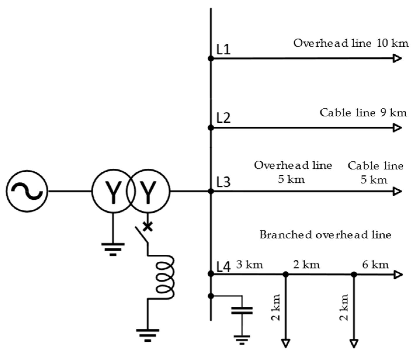
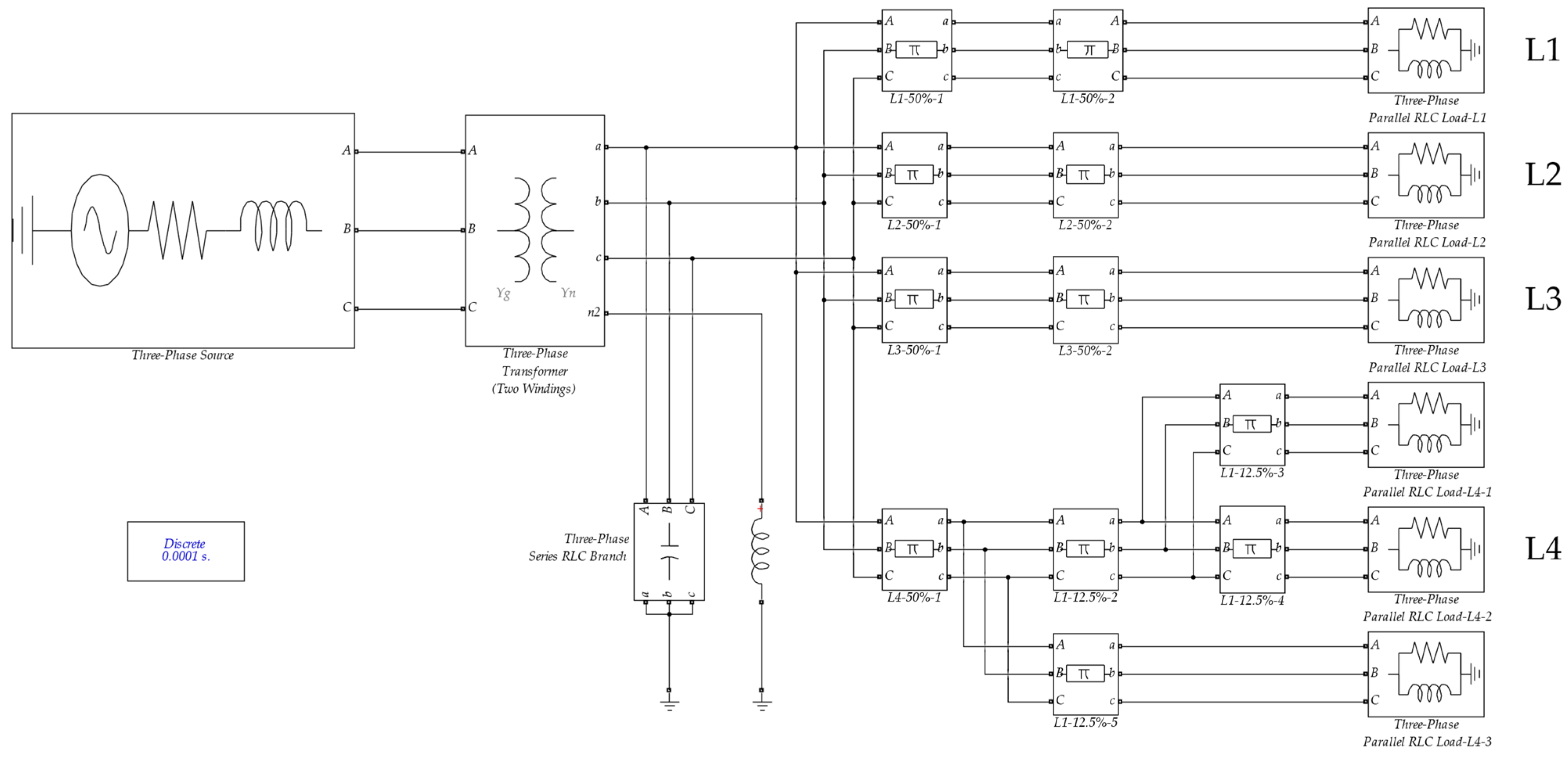
To investigate the transient characteristics of SPG faults in distribution networks, a 10 kV distribution system simulation model is developed using MATLAB/Simulink R2021b (The MathWorks, Natick, MA, USA). The model structure is inspired by EMTP-based configurations reported in the literature and comprises a 110/10.5 kV transformer, four feeder branches, and representative loads. For the purposes of simulation and parameter control, three equivalent transmission lines with differing positive- and zero-sequence impedances are implemented on the 10 kV bus side. At the terminal of each line, parallel RLC loads are connected to emulate the characteristics of typical industrial and commercial users. The schematic diagram of the SPG fault model is shown in Figure 1, in which the feeder topology and grounding resistance configurations are illustrated. In branch L1, the “Three-Phase Parallel RLC Load” block in Simulink is utilized, with the connection type configured as grounded Y (wye). The rated phase voltage is specified as 10 kV, with an active power of 249 kW and a reactive inductive power of 15.7 kvar. The system is operated at a nominal frequency of 50 Hz. These configurations are implemented in Figure 2, which presents the Simulink implementation of the system model. Line lengths and electrical parameters, such as inductive reactance and susceptance, are assigned based on models referenced from previous studies.

2.1.1. Fault and Load Condition Configuration

To evaluate the model’s capability in capturing transient characteristics, the simulation is configured with a fault initiation time of 0.005 s, a fault duration of 0.005 s, a total simulation time of 0.02 s, and a sampling frequency of 10 kHz. SPG faults are introduced at multiple locations along feeder L1, specifically 5 km from the bus, under two grounding resistance levels ($R_{\mathrm{f}}$ = 10 Ω and 50 Ω), to simulate varying fault intensities. The load access ratio’s impact on the transient response is also considered, with representative load conditions of 20%, 50%, and 80% loading at the ends of each feeder. The system’s zero-sequence current is monitored for each condition to analyze its transient behavior under varying fault and loading scenarios. Symmetrical three-phase parallel RLC loads are used at each feeder endpoint, grounded using a Y-connection to emulate realistic industrial and commercial loads. For example, on branch L1, the phase-to-phase voltage is maintained at 10 kV, and the system frequency is held at 50 Hz. The load is inductive, with no capacitive component. Simulink blocks are configured to extract branch voltage and current signals, supporting feature extraction and transient response analysis. These configurations reflect the steady-state power characteristics of real-world distribution networks, ensuring the simulation’s engineering relevance and fidelity.

2.1.2. Data Preparation and Description

The dataset for model training and evaluation is generated based on the previously described simulation setup. Each data sample includes labeled voltage and current signals collected under various fault scenarios, such as different grounding resistances (10 Ω and 50 Ω), fault locations, and load access ratios (20%, 50%, and 80%). The choice of 10 Ω as the minimum and 50 Ω as the maximum grounding resistance explicitly reflects the contrast between low-impedance faults, which result in higher fault currents and stronger transients, and high-impedance faults, which produce weaker currents but are more challenging to detect. Likewise, varying the fault locations enables the analysis of how electrical distance from the source influences signal attenuation and distortion, ensuring coverage of both near-bus and remote scenarios [41]. Additionally, feeder characteristics, including impedance variations and branch-specific loads, are considered to capture a wide range of operational conditions. The collected signals are preprocessed by removing baseline drift, normalizing amplitudes, and segmenting them into uniform time windows. Each segment is labeled with its fault type and location, ensuring the dataset is well-suited for supervised learning tasks.

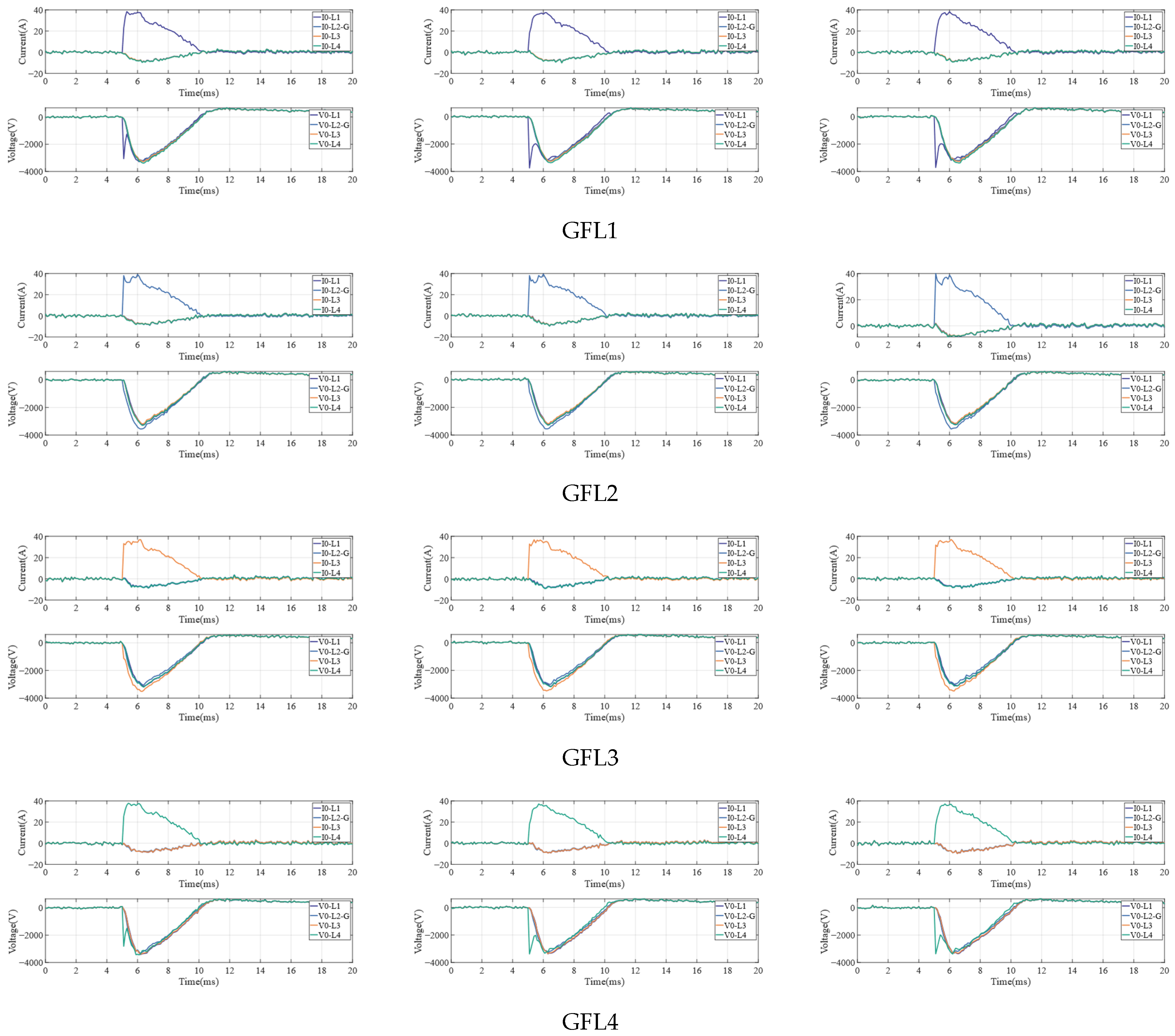
A representative sample from the dataset is shown in Figure 3, in which typical zero-sequence current waveforms under various single-phase grounding fault conditions are illustrated. Each waveform is associated with a distinct simulation configuration, characterized by variations in fault location, grounding resistance, and load access ratio. Specifically, the samples labeled GFL1 to GFL4 are associated with scenarios in which ground faults are applied to different feeder lines (L1 to L4). The label “GFLx” is defined to represent a Ground Fault on Line x, where the numeric suffix (1–4) is used to distinguish the specific line on which the fault is introduced. This subset is intended to demonstrate the diversity of faulted line scenarios and the comprehensiveness of the simulation configurations. The dataset has been systematically constructed to facilitate data-driven analyses of transient characteristics, as well as to support fault identification, localization, and classification tasks.

2.2. Feature Engineering

In the detection of SPG faults in three-phase four-wire systems (including phases A, B, C, and a neutral point), accurate and efficient judgment relies on the collection, fusion, and analysis of various current and voltage eigenvalues from each phase. When an SPG fault occurs, multiple eigenvalues of current and voltage change, including time-domain features such as mean, standard deviation, maximum/minimum values, peak-to-peak value, skewness, and mean absolute deviation; frequency-domain features such as spectral centroid, spectral entropy, spectral bandwidth, skewness, and peak value; wavelet features such as wavelet entropy, energy of each wavelet decomposition layer, and wavelet packet node energy; and waveform shape features such as main peak width, number of peaks, average peak amplitude, and maximum peak amplitude. For single-phase fault detection, it is essential to extract voltage and current eigenvalues from each line of the three-phase four-wire system as the main basis for fault assessment, despite the high computational complexity involved. In this study, for identifying SPG faults in three-phase four-wire transmission systems, multi-dimensional eigenvalues are weighted and fused into an eigenvalue table for clear data presentation. The TabNet model is then used to process data in the eigenvalue table to determine the location and severity of the SPG fault.

Step 1. Twenty-four types of waveform data from eight channels (G1–G4 current and G1–G4 voltage) under six different fault conditions ($R_{\mathrm{f}}$ = 10 Ω/50 Ω; fault positions = 20%, 50%, 80%) are preprocessed, including de-mean and normalization, smoothing (Savitzky–Golay filtering), and main peak alignment.

Step 2. The L2-norm is employed to evaluate and rank the importance of multi-domain features in the classification of SPG faults. The top 20 features with the highest L2-norm values are selected as representative inputs to construct the final feature dataset.

Step 3. To further reduce computation and improve system performance, multimodal feature fusion is performed on the eigenvalue data. Specifically, 24 types of waveform eigenvalue data from eight channels under six different fault states are fused simultaneously to form one channel.

Step 4. The TabNet model is used to process data samples after multimodal feature fusion. Meanwhile, the same data are processed by Support Vector Machine (SVM), CNN, Long Short-Term Memory (LSTM), and Transformer models. The superiority of the TabNet model is demonstrated through five performance metrics: Accuracy, Kappa, Macro-F1, classification report, and confusion matrix.

2.2.1. Data Preprocessing

In the detection of SPG faults, data preprocessing is necessary to remove noise, correct distortion, and normalize feature scales. These steps ensure that multi-channel signals are properly aligned and that extracted features are enhanced for better discrimination. The ultimate goal is to provide clean and consistent inputs that improve the robustness and accuracy of the model. Its core is to denoise current and voltage waveform signals, correct their distortion, unify data formats, and improve the purity and analyzability of fault signals. Specifically, it includes suppressing high-frequency noise (e.g., wavelet threshold denoising) to eliminate white noise and impulse interference; and imputing missing values and correcting outliers to ensure waveform continuity and rectify distortion.

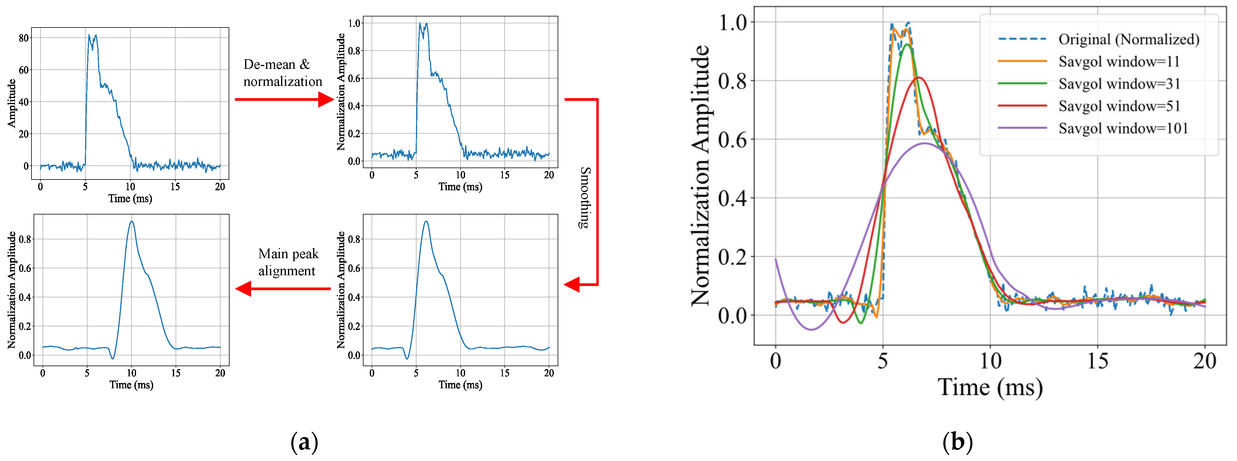
The original waveform signals are standardized and filtered, as shown in Figure 4a, Demeaning eliminates the DC offset of the signal to prevent baseline drift caused by CT/PT zero drift from distorting feature quantities. Normalization, used when fault currents in different lines vary significantly, eliminates the influence of magnitude, unifies the amplitude scale, and enhances model generalization. Smoothing involves using the Savitzky–Golay filtering method to smooth waveform data, which, compared with common methods like moving average filtering and wavelet denoising, offers advantages of no phase delay, minimal edge distortion, and high computational efficiency, accurately retaining and extracting features of transient pulses (e.g., Max Peak, Impulse Factor), avoiding distortion of Peak Width, Bandwidth, etc., caused by waveform time shift after filtering, and effectively removing random oscillations (2–5 kHz high-frequency burrs) in arc grounding, as shown in Figure 4b. Main peak alignment unifies the fault initiation time to eliminate propagation delay differences (μs-ms level) during faults in different lines, ensuring no window misalignment in feature extraction.

2.2.2. Feature Extraction

In diagnosing SPG faults in three-phase four-wire systems, a fault event leads to changes in multiple multi-dimensional voltage and current features across the four lines. As summarized in

Table 1. Overview of Extracted Features and Mathematical Expressions.

Feature Name	Mathematical Expression	Feature Name	Mathematical Expression
STD	$\sigma =\sqrt{{\displaystyle \frac{1}{N}}{\displaystyle \sum {(x_i-\mu )}^2}}$	Spectral Centroid	${\displaystyle \frac{{\displaystyle \sum f_i}·\left|P_i\right|}{{\displaystyle \sum \left|P_i\right|}}}$
Max	$\max (x_i)$	Spectral Entropy	$-{\displaystyle \sum (P_i·{\log }_2(P_i)})$
Min	$\min (x_i)$	Bandwidth	$\sqrt{{\displaystyle \sum {(f_i-\mu )}^2·}{P}_i}$
PTP	$\max (x_i)-\min (x_i)$	Spectral Variance	$Var(X_f)$
Skewness	${\displaystyle \frac{1}{N}}{\displaystyle \sum (}{\displaystyle \frac{(x_i-\mu )}{\sigma }}{)}^3$	Spectral Skewness	${\displaystyle \frac{1}{N}}{\displaystyle \sum (}{\displaystyle \frac{(f_i-\mu )}{\sigma }}{)}^3$
Kurtosis	${\displaystyle \frac{1}{N}}{\displaystyle \sum (}{\displaystyle \frac{(x_i-\mu )}{\sigma }}{)}^4$	Spectral Kurtosis	${\displaystyle \frac{1}{N}}{\displaystyle \sum (}{\displaystyle \frac{(f_i-\mu )}{\sigma }}{)}^4$
Crest Factor	${\displaystyle \frac{\max (|x_i|)}{rms}}$	Wavelet Entropy	$-E_i·\log (E_i)$
Impulse Factor	${\displaystyle \frac{\max (|x_i|)}{\mathrm{mean}(|x_i|)}}$	Wavelet Energy L1~L4	${\displaystyle \sum (c_i}{)}^2$
Peak Width	$h_{peak}=h_{peak}-P\ast R$	Wpe node 0~7	${\displaystyle \sum (c_i}{)}^2$
Mean Peak Amplitude	$mean(x_{[peak]})$	IQR	$Q_3-Q_1$

, the extracted features span time-domain, frequency-domain, waveform, and wavelet perspectives, including interquartile range (IQR), standard deviation (STD), mean absolute deviation (MAD), interpeak value (PTP), wavelet packet node energy (WPN), and wavelet decomposition layer energy (WE). These descriptors are closely aligned with SPG fault mechanisms: arc faults produce sharp transients that elevate kurtosis and crest factor; unbalanced or capacitive grounding introduces waveform asymmetry reflected in skewness; spectral centroid and entropy characterize the redistribution of spectral energy under high resistance; and wavelet-based measures emphasize localized transient responses. Collectively, these features capture both statistical properties and physical fault signatures, ensuring that the extracted set provides a comprehensive and interpretable representation of SPG fault characteristics. Input multiple multi-dimensional features into a linear model based on L2 norms for weight sorting and screen out the top 20 most important feature values in the judgment of single-phase grounding faults. The L2 norm-based linear model quantifies feature importance through the L2 norm of the weight vector of the linear model—the larger the absolute value of the weight, the higher the contribution of the feature to fault discrimination. The expression of the linear model is as follows:

$$y=w_0+w_1{x}_1+w_2{x}_2+\dots +w_{20}{x}_{20}$$

(1)

where $y$ is the fault state label (usually, $y=0$ represents the normal state, and $y=1$ represents the fault state), $x_i$ is the ith feature (up to 20 features), and $w_i$ is the feature weight, which is used to measure feature importance.

Meanwhile, it is necessary to impose a constraint on the L2 norm, i.e., L2 regularization (Ridge regression):

$$\underset{w}{\min }(||y-X_w|{|}_2^2+\alpha ||w|{|}_2^2)$$

(2)

where $\alpha$ is the regularization strength, which controls weight decay. $\left|w_i\right|$ can directly reflect the feature’s ability to judge faults. After the linear model based on the L2 norm screens and ranks the features in terms of importance, the top 20 features in terms of importance are selected, as shown in Figure 5. The fused dataset is composed of 59 features extracted from time-domain, frequency-domain, wavelet-based, and statistical descriptors. To ensure reliable feature representation, all features are ranked according to their L2 norm values, by which their overall contributions across samples are quantified. Figure 5a illustrates that model performance (accuracy, macro-F1, and kappa) steadily improves as the number of selected features increases, but reaches a plateau once 20–30 features are included. This demonstrates that additional features beyond this range contribute little new information and mainly introduce redundancy. Therefore, the top 20 features are selected, as they preserve sufficient discriminative information while maintaining compactness and interpretability. These selected features collectively capture diverse aspects of the signal, ensuring both relevance and complementarity in the fused feature space, while providing a stable, data-driven basis for model training and improving classification accuracy.

They are presented in Figure 5b and measure the magnitude of each feature vector across all samples. Features with higher L2 norms are considered to carry more discriminative power for fault classification. The most important features include kurtosis, skewness, and IQR, highlighting their strong relevance in capturing signal shape and distribution. Several wavelet-based features, such as wavelet entropy, wavelet energy from different decomposition levels, and WPN are also highly ranked, indicating their effectiveness in representing time-frequency characteristics of fault signals. Additionally, statistical indicators like crest factor, MAD, and STD are selected for their ability to reflect signal amplitude and fluctuation. These selected features collectively capture diverse aspects of the signal, ensuring both relevance and complementarity in the fused feature space, while providing a stable, data-driven selection process that preserves high-impact information for model training and improves classification accuracy.

Figure 6 further validates the necessity of the proposed feature selection strategy by comparing the performance of the Top-20 features with that of randomly selected feature subsets of the same size. As shown in Figure 6a–c, the Top-20 features consistently achieve significantly higher scores in terms of kappa coefficient, macro-F1, and accuracy, while also exhibiting lower variance across repeated trials. In contrast, the Random-20 subsets produce unstable and substantially weaker results, highlighting the risk of relying on arbitrary feature combinations. These findings confirm that the proposed L2 norm-based selection not only captures the most informative and complementary features but also ensures robustness and reproducibility. Therefore, feature selection is a necessary step: it reduces redundancy, enhances interpretability, and guarantees that the retained features contribute directly to accurate and stable fault classification.

2.2.3. Multimodal Feature Fusion

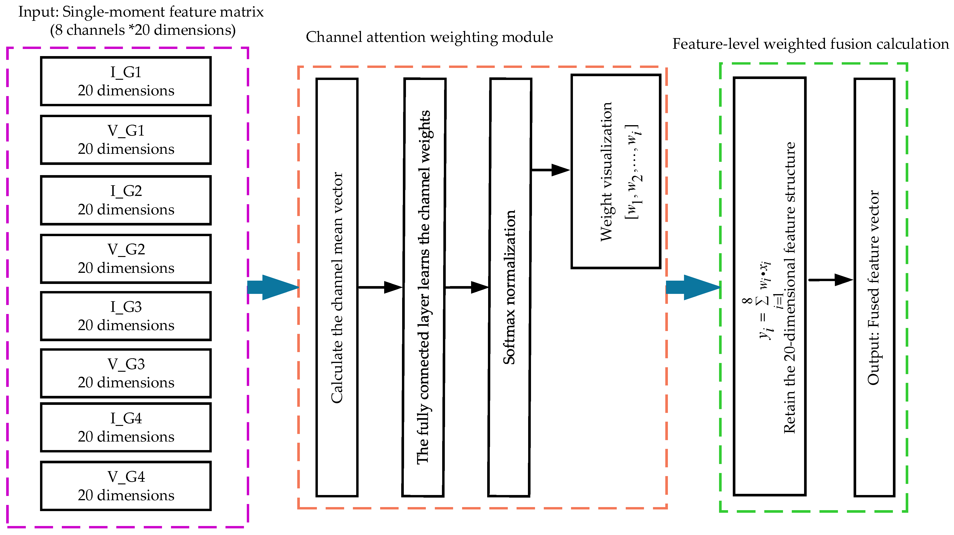
For each fault instance, voltage and current signals from four feeder lines (L1 to L4) are collected, resulting in eight channels of raw input. Each channel captures a distinct spatial or electrical perspective of the same fault event. However, relying on a single feeder’s data may lead to incomplete or biased interpretation, especially under weak fault signals or noise. By fusing all eight channels, the model can leverage complementary and redundant patterns across lines, thus improving fault type discrimination and overall robustness. To effectively integrate information from all eight channels, a feature-level weighted fusion module is designed, as illustrated in Figure 7. The input is a single-moment feature matrix comprising eight channels, each with 20 dimensions, derived from the voltage and current signals of four feeder lines. The detailed channel configuration is summarized in

Table 2. Input and structure.

Dimension	Explanation	Size
Time	At the same sampling moment	$t_k$
Passage	8 channels	8
Feature	The 20-dimensional features after screening	20
Data block	8-channel feature matrix at a single moment	8 × 20

.

First, the channel attention weighting module computes the mean vector for each channel to capture global channel-level statistics. These mean vectors are then passed through a fully connected layer followed by a SoftMax function to generate normalized channel attention weights:

$$[w_1,w_2,\dots ,w_8],\mathrm{where}{\displaystyle \sum _{j=1}^8{w}_j}=1$$

(3)

These learned weights reflect the significance of each channel in the context of fault classification. Next, the feature fusion is performed by applying the learned weights to the corresponding feature channels using a weighted sum:

$$y_i={\displaystyle \sum _{j=1}^8{w}_j}\cdot x_{ij}$$

(4)

where $x_{ij}$ denotes the element of the $j\text{-}\mathrm{th}$ channel, and $y_i$ is the $j\text{-}\mathrm{th}$ element of the final fused feature vector. This operation retains the 20-dimensional structure while adaptively emphasizing informative channels. The resulting fused feature vector captures the complementary information across all feeders, enhancing the model’s ability to generalize across various fault conditions.

3. Model Design

3.1. Overview of the TabNet Model

TabNet is a deep learning architecture specifically designed for tabular data. Unlike conventional deep neural networks that often struggle with structured inputs, TabNet employs a sequential attention mechanism that adaptively focuses on the most informative features for each sample. This design not only improves classification performance but also provides interpretability by identifying the contribution of individual features. In grounding fault diagnosis, where the data are high-dimensional and heterogeneous, these characteristics make TabNet particularly suitable. While TabNet itself is not entirely new, the novelty of this work lies in its tailored adaptation to single-phase grounding (SPG) fault detection. We integrate feature fusion with L2 norm-based feature selection to enhance interpretability, and employ Optuna-driven hyperparameter optimization to improve stability and robustness. This integrated framework enables TabNet to achieve superior generalization and reliability under complex fault scenarios in three-phase four-wire distribution systems.

One of TabNet’s key innovations is its ability to perform instance-wise feature selection via an attention mechanism. At each decision step $i$, the model computes a feature mask $M^{[i]}\in {ℝ}^{B\times D}$, where $B$ is the batch size and $D$ is the number of features. The mask is derived as

$$M^{[i]}=\mathrm{sparsemax}\left(P^{[i-1]}\cdot h_i\left(a^{[i-1]}\right)\right)$$

(5)

where $a^{[i-1]}$ is the activation from the previous step, $h_i(\cdot )$ is a trainable transformation that transforms the input features, usually consisting of a fully connected layer followed by batch normalization. The term $P^{[i-1]}$ serves as a prior, helping the model decide how much to reuse features from earlier steps. The use of Sparsemax ensures that only the most relevant and important features are passed to the next step, while irrelevant ones are suppressed. The selected features at each decision step $i$ are obtained by applying the learned mask $M^{[i]}$ to the input feature vector $f$, resulting in a filtered representation $M^{[i]}\cdot f$. This masked input is then passed through a feature transformer, which outputs two branches: $d^{[i]}$ is a decision vector, contributing to the final model output, and $a^{[i]}$ is an activation vector, serving as input to the next decision step. This step-wise design enables the model to focus on different subsets of features at each stage. After completing all $N_{\mathrm{steps}}$ decision steps, the outputs $d^{[i]}$ from each step are aggregated using a ReLU activation to form the final decision embedding:

$$d_{\mathrm{out}}={\displaystyle \sum _{i=1}^{N_{\mathrm{steps}}}\mathrm{ReLU}}(d^{[i]})$$

(6)

This cumulative representation is then passed to the output layer for prediction.

The architecture of the TabNet model, designed to capture and process feature interactions for effective learning, is illustrated in Figure 8. The model consists of three key steps. In Step 1, the input features are processed through a Feature Transformer, where they are split and. Then an Attentive Transformer is involved in Step 2 to generate attention masks that guide feature selection. In Step 3, the outputs are aggregated to form an intermediate feature representation. A detailed view of the Feature Transformer is shown in Figure 8b, which highlights the layers shared across decision steps and those specific to each step, allowing the model to learn both generalizable and task-specific features. Figure 8c provides a detailed view of the Attentive Transformer, where prior scales are integrated, and the Sparsemax activation function is used to generate sparse attention masks. This approach allows the model to focus on key features, improving feature selection and overall performance.

3.2. Hyperparameter Optimization

To optimize the TabNet model’s performance, this study employs Optuna [42], a lightweight and flexible hyperparameter optimization framework. Optuna formulates the tuning process as a black-box optimization problem:

$${\theta }^{*}=\arg \underset{\theta \in \Theta }{\max }f(\theta )$$

(7)

where ${\theta }^{*}$ is the activation from the previous step, $h_i(\cdot )$ is a trainable transformation that denotes a set of hyperparameters, $f(\theta )$ is the objective function, and $\Theta$ is the search space. Adaptive samplers, such as the Tree-structured Parzen Estimator (TPE), are used to efficiently explore the search space and incorporate early stopping (pruning) to terminate unpromising trials. The process begins by defining an objective function that quantifies model performance (e.g., validation accuracy or loss) for a given set of hyperparameters.

The complete search ranges of the candidate hyperparameters are summarized in

Table 3. Ranges of Candidate Hyperparameters.

Hyperparameter	Learning Rate	Decision Width	Attention Width	Number of Decision Steps	Gamma	Sparse Regularization
Search range	Log-uniform [1 × 10−4, 1 × 10−1]	32–256	16–128	{3, 5, 7, 9}	1.0–2.5	Log-uniform [1 × 10−5, 1 × 10−2]
Hyperparameter	Batch size	Optimizer	Training epochs	Early stopping patience	Learning rate decay
Search range	{128, 256, 512}	Adam (β1 = 0.9, β2 = 0.999)	200	20 epochs	0.5 if no improvement in 30 epochs

. These hyperparameters are selected because they represent the key factors that determine the trade-off between model accuracy, interpretability, and generalization. Specifically, the decision width (n_d) and attention width (n_a) define the dimensionality of the decision and attention embeddings, thereby controlling the representational power of the model. The number of decision steps (n_steps) governs how many sequential feature selection processes are performed, which determines the depth of information extraction. The relaxation parameter ($\gamma$) adjusts the extent of feature reuse across different steps, where larger values encourage overlap and smaller values promote diversity. The sparsity regularization coefficient ($\lambda$ sparse) imposes sparsity on the attentive masks, enhancing interpretability while mitigating overfitting. Finally, the learning rate is included because it directly affects optimization speed and stability.

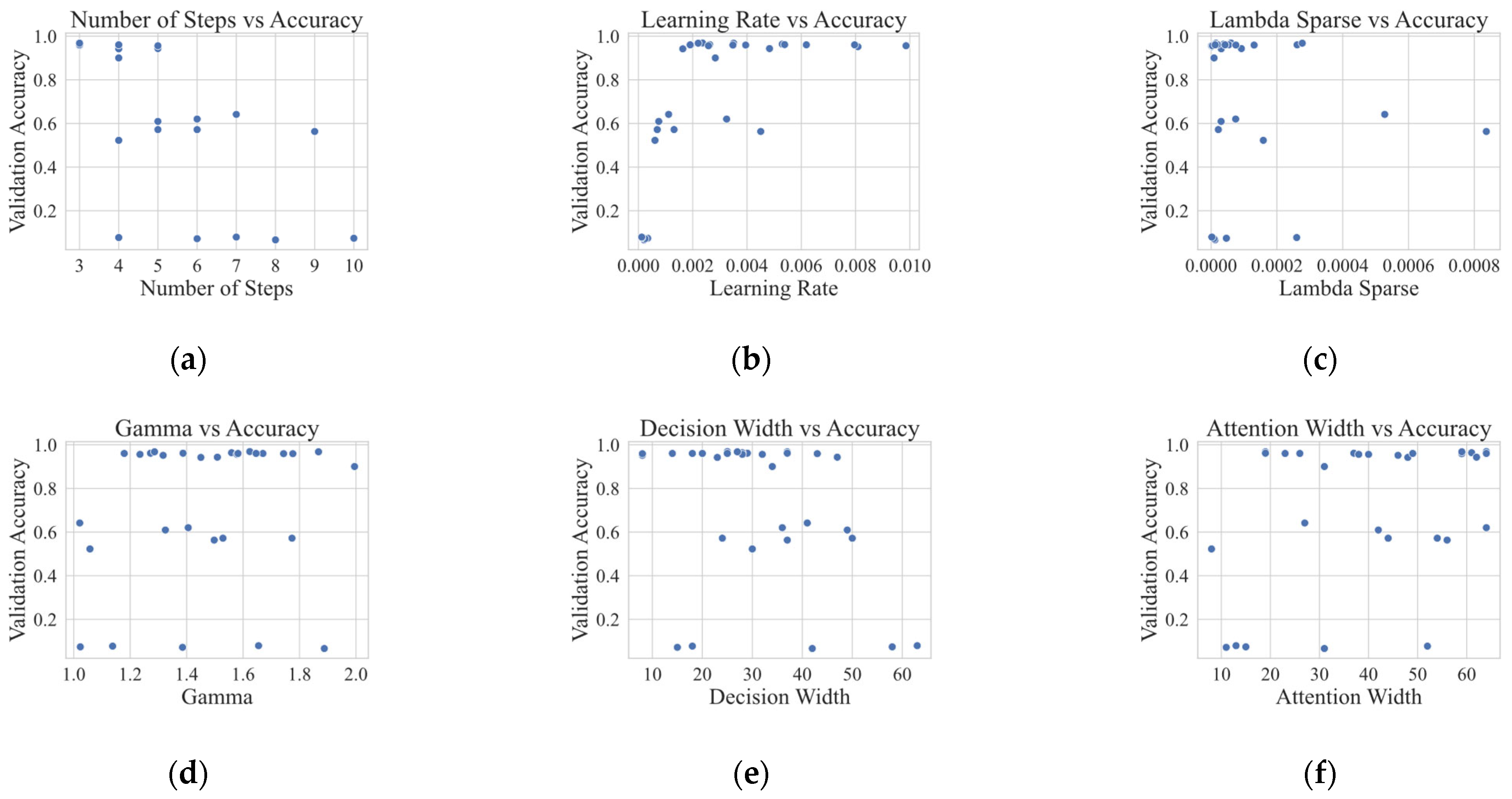
By incorporating these hyperparameters into the search space, both structural design parameters (n_d, n_a, n_steps, $\gamma$, $\lambda$ sparse) and training dynamics (learning rate) are jointly optimized. As illustrated in Figure 9, the learning rate and decision width exhibit strong sensitivity, with optimal performance consistently achieved within narrow ranges. Similarly, the number of decision steps and attention width substantially affect accuracy, confirming their critical role in determining model capacity and representation power. In contrast, $\gamma$ and $\lambda$ sparse show relatively weaker but still noticeable effects, suggesting that they contribute to overall model generalization rather than dominating performance. As summarized in

Table 4. Optimal Parameters of the Proposed Model.

Decision Width	Attention Width	Decision Steps	Gamma	Lambda Sparse
18	26	3	1.67	2.61 × 10−4
Learning rate	Batch size	Optimizer	Max epochs	Early stopping patience
1.94 × 10−3	64	Adam	200	20 epochs

, the final optimal configuration obtained from Optuna achieves a balanced trade-off: moderate widths (n_d = 32, n_a = 24) capture sufficient discriminative information without redundancy, n_steps = 7 enables deeper sequential feature selection, $\gamma$ = 1.5 provides moderate feature reuse, and $\lambda$ sparse = 1 × 10⁻⁴ enforces an interpretable level of sparsity. A learning rate of 0.006 stabilizes convergence and avoids oscillations. Collectively, these optimized values reflect a configuration that balances accuracy, robustness, and interpretability, and this configuration is consistently adopted in all subsequent experiments.

The effects of hyperparameter optimization on model performance and inter-parameter relationships are further illustrated in Figure 10. As shown in Figure 10a, a correlation heatmap reveals the pairwise relationships between hyperparameters and validation accuracy. Notably, the learning rate and number of steps show strong positive and negative correlations with validation accuracy, respectively, indicating their crucial roles in model generalization. Other parameters, such as attention width and decision width, also exhibit moderate correlations, suggesting they contribute to the model’s capacity and attention mechanism strength. In Figure 10b, the recall scores of some previously low-performing classes show significant improvements. This demonstrates the effectiveness of Optuna-based optimization in enhancing classification robustness and addressing class imbalance to some extent. These results demonstrate that careful tuning of key parameters, such as the learning rate, number of decision steps, and feature selection width, not only enhances the model’s predictive accuracy but also strengthens its robustness in handling imbalanced fault categories.

4. Results and Analysis

This section presents the experimental results and discussion based on the optimized TabNet model applied to the collected grounding fault dataset. The model’s performance is evaluated using multiple metrics and compared against several baseline methods: Gao et al. use TCN for grounding fault detection in distribution systems [28], Teimourzadeh et al. employ a CNN-LSTM framework to capture both spatial and temporal fault characteristics [29], Fanim et al. introduce CNSF to enhance feature extraction for complex fault patterns [30], and Gao et al. propose a Dual-Branch CNN to extract complementary features from upstream and downstream zero-sequence currents, showing strong robustness under resonant grounding conditions [31]. As shown in Figure 11a, the per-class precision of TabNet remains consistently high across all 24 fault categories, demonstrating its superior reliability and stability at the class level. In contrast, the baseline models, particularly TCN and CNN-LSTM, show drops in precision for certain classes such as class 10, 14, and 16, indicating challenges in handling complex or imbalanced fault conditions. Figure 11b compares the overall performance of all models using three key evaluation metrics: accuracy, kappa coefficient, and macro-F1 score. The optimized TabNet model surpasses all baselines, achieving an accuracy of 0.9733, a kappa coefficient of 0.9721, and a macro-F1 score of 0.9739. These results confirm the superior generalization ability of TabNet and its effectiveness in accurately classifying diverse grounding fault types. To mitigate the effect of randomness, all models are evaluated under a 5 × 5 stratified cross-validation scheme with multiple independent runs. Mean values, standard deviations, and 95% confidence intervals (CIs) are reported. Furthermore, pairwise Wilcoxon signed-rank tests are conducted to ensure that the observed improvements are statistically significant.

The training dynamics of all evaluated models are shown in Figure 12. Figure 12a demonstrates that the optimized TabNet model exhibits smooth convergence, with steadily decreasing loss and consistently improving accuracy, indicating efficient and robust learning behavior. In contrast, CNSF in Figure 12b shows larger fluctuations in both loss and accuracy, reflecting sensitivity to class imbalance and unstable convergence. Figure 12c illustrates the TCN model, which converges rapidly in the early epochs but plateaus later, suggesting limited capacity to capture more complex patterns. Figure 12d presents the CNN+LSTM model, which achieves fast convergence but also shows oscillations and early saturation. Finally, the Dual-Branch CNN in Figure 12e reaches high training accuracy but displays a small gap between training and test performance, indicating mild overfitting. Overall, TabNet achieves the most stable and reliable training dynamics, highlighting its superior generalization ability in SPG fault classification tasks.

To ensure the robustness of the comparative analysis, a comprehensive evaluation protocol is adopted that integrates cross-validation, confidence interval estimation, and statistical hypothesis testing. Reporting only mean accuracy may conceal randomness and uncertainty, whereas statistical testing verifies whether improvements are consistently significant rather than incidental. All models are repeatedly evaluated under a 5 × 5 stratified K-fold cross-validation scheme, which balances class distributions in each fold and reduces variance from random partitioning.

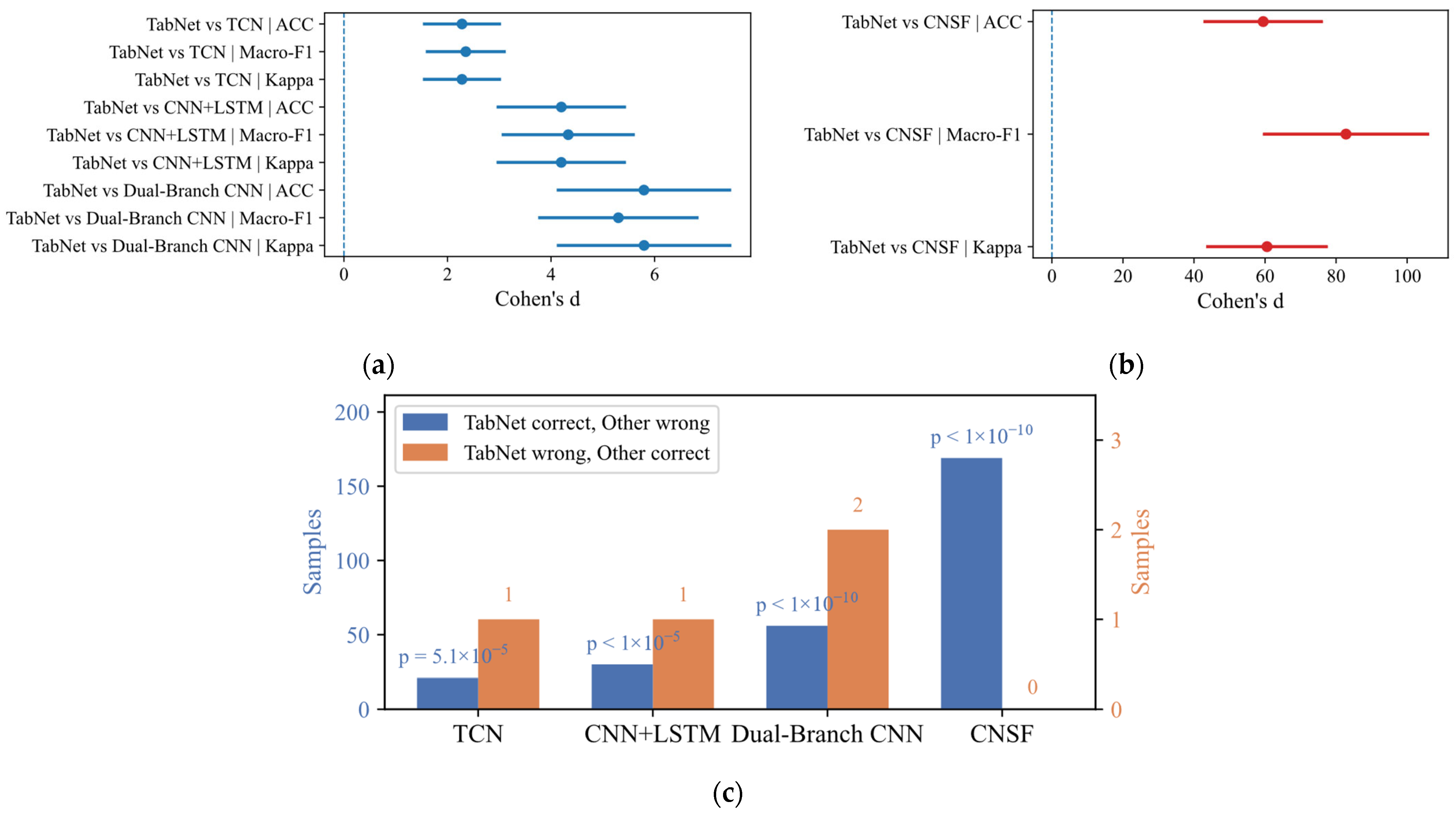
As summarized in

Table 5. Overall Metrics with 95% CI.

Model	ACC Mean	ACC Std	ACC 95CI Low	ACC 95CI High	MacroF1 Mean	MacroF1 Std
CNN+LSTM	0.788825	0.039645	0.773987	0.803957	0.761206	0.044243
CNSF	0.074038	0.008793	0.070587	0.077255	0.011408	0.001425
Dual-Branch CNN	0.699831	0.044033	0.681541	0.715244	0.663003	0.054775
TCN	0.872985	0.032169	0.859752	0.884748	0.863229	0.033098
TabNet	0.956007	0.009307	0.952348	0.959447	0.953119	0.010848
Model	MacroF1 95CI Low	MacroF1 95CI High	Kappa Mean	Kappa Std	Kappa 95CI Low	Kappa 95CI High
CNN+LSTM	0.744544	0.777988	0.779627	0.041384	0.764133	0.795413
CNSF	0.010842	0.011917	0.035518	0.008391	0.032231	0.038528
Dual-Branch CNN	0.639858	0.682870	0.686808	0.045916	0.667757	0.702888
TCN	0.849404	0.875307	0.867452	0.033572	0.853644	0.879727
TabNet	0.948820	0.957188	0.954089	0.009712	0.950270	0.957679

Mean and 95% bootstrap confidence intervals (5 × 5 stratified CV). CIs are obtained by 10,000 bootstrap resamples from fold-wise scores.

, the optimized TabNet model achieves the best overall performance, with ACC = 0.9560 ± 0.0093 (95% CI: 0.9523–0.9594), Macro-F1 = 0.9531 ± 0.0108, and Kappa = 0.9541 ± 0.0097. These results demonstrate not only high accuracy but also remarkable stability, as reflected by the narrow confidence intervals. In contrast, TCN reaches 0.8730 ± 0.0322, CNN+LSTM achieves 0.789 ± 0.0396, and Dual-Branch CNN attains 0.700 ± 0.0440, while CNSF performs very poorly at 0.074 ± 0.0088. To further validate these findings, Figure 13 presents statistical comparisons between TabNet and the baselines. Figure 13a,b display forest plots of Cohen’s d effect sizes, showing consistently large to very large margins for TabNet, especially against CNSF, while Figure 13c illustrates McNemar’s test, where asymmetric counts (21 vs. 1 for TCN, 30 vs. 1 for CNN+LSTM, 56 vs. 2 for Dual-Branch CNN, and 169 vs. 0 for CNSF) again yield highly significant p-values (<1 × 10⁻⁵). Collectively, Table 5 and Figure 13 provide strong and complementary evidence that TabNet not only achieves higher accuracy but also delivers significantly more reliable and generalizable performance than all baseline models.

To further demonstrate interpretability, Figure 14 provides a multi-perspective visualization of the attention distributions learned by TabNet across different fault categories. Panel Figure 14a shows the class-wise heatmap of attention scores aggregated over test samples, where distinct feature patterns can be observed for different fault types. For instance, the model consistently attends to kurtosis and skewness in arc-related faults (e.g., Class 10 and Class 14), while wavelet energy and entropy features are more prominent in capacitor grounding conditions (e.g., Class 16). Panel Figure 14b further highlights the top-10 features contributing to a specific arc fault class, verifying that the model prioritizes physically meaningful descriptors such as higher-order statistical moments. In addition to class-level insights, Panels Figure 14c,d quantitatively compare the attention mass allocated to the selected Top-20 features against multiple Random-20 feature groups. The Top-20 set consistently captures a significantly larger proportion of attention, with tighter and more stable distributions, thereby validating the robustness and discriminative power of the chosen features. These results confirm that TabNet does not merely rely on spurious correlations but adaptively emphasizes fault-relevant features in alignment with electrical and physical fault mechanisms. Together, these visualizations provide essential evidence for the interpretability of the proposed method. They show that the model’s decision-making is not a black box but is grounded in domain-relevant features, which is critical for building practitioner trust and for enabling practical deployment in real-world fault diagnosis of distribution networks.

5. Limitation and Discussion

Despite the promising performance of the proposed method, several limitations should be acknowledged. First, the dataset used in this study is primarily based on simulated signals, which may not fully capture the noise, nonlinearity, and uncertainties present in real-world distribution networks. Although the simulation model includes multiple grounding resistances, load levels, and fault locations, more complex fault scenarios, such as high-impedance grounding and intermittent arc-ground faults, have not yet been thoroughly validated. Second, while the use of Optuna enables efficient automated hyperparameter optimization, the computational cost is relatively higher compared with conventional tuning methods, which could pose challenges for large-scale or real-time applications. Finally, the performance of TabNet is partly dependent on the quality and stability of feature extraction; in extremely noisy environments, further robustness enhancement may be necessary.

Future work will focus on extending the approach to real-time monitoring environments and enhancing adaptability to complex scenarios, such as systems with distributed energy resources or high-noise conditions.

6. Conclusions

This study introduces a comprehensive framework for SPG fault identification in three-phase four-wire distribution systems, utilizing TabNet and Optuna. By combining simulation models with feature fusion, the method achieves efficient and accurate fault detection. Beyond directly applying deep learning, the proposed framework incorporates several innovations: at the data level, features are extracted from time, frequency, waveform, and wavelet domains to form a multi-domain fusion representation; at the model level, the sparse attention mechanism of TabNet enables both effective learning from tabular data and enhanced interpretability; at the optimization level, Optuna provides automated and efficient hyperparameter tuning compared with traditional grid search or manual adjustment; and at the result level, the approach not only improves classification accuracy but also offers interpretability through attention distribution and feature-level comparisons. These advantages distinguish the proposed framework from existing methods and highlight its robustness and practical value for SPG fault diagnosis. The key findings from this research are summarized as follows:

(1)

A simulation model of a 10 kV distribution system is developed in Simulink to generate diverse SPG fault scenarios under varying grounding resistances, fault locations, and load conditions, resulting in a dataset covering 24 distinct fault categories, with signals collected from eight channels (L1–L4 voltage and current).

(2)

Features are extracted from each channel and fused using an attention-based mechanism. The top 20 informative features are selected using the L2 norm to enhance representation and reduce redundancy.

(3)

The TabNet model optimized using Optuna achieved an accuracy of 97.33%, a macro F1 score of 97.39%, and a kappa coefficient of 0.9721, outperforming recent advanced models such as TCN, CNN-LSTM, CNSF, and Dual-Branch CNN. These results demonstrate the effectiveness of the proposed method in SPG fault identification.

References

1. He, L.; Li, Y.; Chu, X.; Shuai, Z.; Peng, Y.; Shen, Z.J. Single-phase to ground fault line identification for medium voltage islanded microgrids with neutral ineffectively grounded modes. IEEE Trans. Smart Grid 2022, 13, 4312–4326. [Google Scholar] [CrossRef]
2. Tian, J.Y.; Liu, Y.; Xue, Y.D.; Huang, C. Analysis of zero sequence voltage starting of small current grounding fault line selection device. Distrib. Util. 2022, 39, 54–60. [Google Scholar]
3. Qin, S.Y.; Xue, Y.D.; Liu, L.Z.; Guo, Y.; Xu, M. Transient characteristics and influence of small current grounding faults in active distribution network. Trans. China Electrotech. Soc. 2022, 37, 655–666. [Google Scholar]
4. Dong, L.; Qin, S.; Zhang, Z.; Xue, Y.; Xie, D.; Guan, T. Analysis of energy mechanism of high resistance grounding fault in resonant grounding system. Distrib. Util. 2022, 39, 52–58. [Google Scholar]
5. Chen, X.Q.; Gao, W.; Hong, C.; Tu, Y. A novel series arc fault detection method for photovoltaic system based on multi-input neural network. Int. J. Electr. Power Energy Syst. 2022, 140, 108018. [Google Scholar] [CrossRef]
6. Fan, M.; Xia, J.L.; Meng, X.Y.; Zhang, K. Single-phase grounding fault types identification based on multi-feature transformation and fusion. Sensors 2022, 22, 3521. [Google Scholar] [CrossRef] [PubMed]
7. Li, Z.W.; Li, W.J.; Peng, W.X.; Lei, L.; Liang, L.T. Single-phase-to-ground fault line selection method of distribution network based on IHHT-RF. J. Electr. Power Sci. Technol. 2024, 39, 171–182. [Google Scholar]
8. Liang, J. Research on rapid diagnosis method of single-phase grounding fault in distribution network based on deep learning. In Proceedings of the Chinese Automation Congress (CAC), Hangzhou, China, 22–24 November 2019; IEEE: Piscataway, NJ, USA, 2019; pp. 20–24. [Google Scholar]
9. Gao, J.H.; Guo, M.F.; Lin, S.; Chen, D.-Y.; Bai, H. Semantic-segmentation-based approach for early detection and type recognition of single-phase ground fault in resonant distribution networks. Appl. Soft Comput. 2025, 171, 112736. [Google Scholar] [CrossRef]
10. Wang, X.W.; Du, H.; Liang, Z.F.; Guo, L.; Gao, J.; Kheshti, M.; Liu, W. Single phase to ground fault location method of overhead line based on magnetic field detection and multi-criteria fusion. Int. J. Electr. Power Energy Syst. 2023, 145, 108699. [Google Scholar] [CrossRef]
11. Bayati, N.; Balouji, E.; Baghaee, H.R.; Hajizadeh, A.; Soltani, M.; Lin, Z.; Savaghebi, M. Locating high-impedance faults in DC microgrid clusters using support vector machines. Appl. Energy 2022, 308, 118338. [Google Scholar] [CrossRef]
12. Aiswarya, R.; Nair, D.S.; Rajeev, T.; Vinod, V. A novel SVM-based adaptive scheme for accurate fault identification in microgrid. Electr. Power Syst. Res. 2023, 221, 109439. [Google Scholar]
13. Gao, J.; Wang, X.; Wang, X.; Yang, A.; Yuan, H.; Wei, X. A high-impedance fault detection method for distribution systems based on empirical wavelet transform and differential faulty energy. IEEE Trans. Smart Grid 2022, 13, 900–912. [Google Scholar] [CrossRef]
14. Wan, G.F.; Xu, X.K. Research on single-phase grounding detection method in small-current grounding systems based on image recognition. Front. Energy Res. 2024, 12, 1473472. [Google Scholar] [CrossRef]
15. Yang, F.; Li, H.; Hu, W.; Lei, Y.; Chen, H.; Xue, Y. Identification of single-phase line break fault direction based on local voltage information in small current grounding system considering the impact of DG. IEEE Access 2023, 11, 120754–120765. [Google Scholar] [CrossRef]
16. Su, X.N.; Zhang, H.; Gao, Y.W.; Huang, Y.; Long, C.; Li, S.; Zhang, W.; Zheng, Q. The classification model for identifying single-phase earth ground faults in the distribution network jointly driven by physical model and machine learning. Front. Energy Res. 2023, 10, 919041. [Google Scholar] [CrossRef]
17. Zhang, H.; Zhang, D.H.; Liu, N.Y.; Wu, K.; Shi, Z. Single-phase fault line selection method for small current grounding system based on improved VMD and ConvNeXt. High Volt. Eng. 2025, 51, 730–741. [Google Scholar]
18. Li, Y.H.; Li, C.; Cao, W.S. Single-phase grounding fault line selection in resonant grounding system based on MCEEMD-MPE normalization and k-means algorithm. Processes 2025, 13, 2. [Google Scholar]
19. Luo, G.M.; Yang, X.F.; Shang, B.Y.; Luo, S.; He, J.; Wang, X. High-resistance grounding fault detection method in distribution networks based on improved stacked denoising autoencoder. Power Syst. Prot. Control 2024, 52, 149–160. [Google Scholar]
20. Ravi Kumar, J.; Devaraj, D.; Vinodh Kumar, D.M. Adaptive variational mode decomposition-based deep random vector functional link network for fault classification and location in PV integrated DC microgrids. Appl. Soft Comput. 2022, 121, 108731. [Google Scholar]
21. Guo, M.; Lin, H.; Lin, J.; Hong, Q. Synthetic zero-sequence signal-based intelligent location method for single-phase ground fault in distribution networks. IEEE Trans. Instrum. Meas. 2025, 74, 1–13. [Google Scholar] [CrossRef]
22. Zhao, P.; Wang, Y.; Wang, L.; Wei, J. A graph neural network-based approach for voltage transformer fault diagnosis with wavelet threshold denoising. Meas. Sci. Technol. 2025, 36, 086107. [Google Scholar]
23. Alhanaf, A.S.; Farsadi, M.; Balik, H.H. Fault detection and classification in ring power system with DG penetration using hybrid CNN-LSTM. IEEE Access 2024, 12, 59953–59975. [Google Scholar] [CrossRef]
24. Alaca, O.; Ekti, A.R.; Wilson, A.; Snyder, I.; Stenvig, N.M. CNN-based phase fault classification in real and simulated power systems data. In Proceedings of the IEEE Power & Energy Society General Meeting (PESGM), Seattle, WA, USA, 21–25 July 2024; pp. 1–5. [Google Scholar]
25. Gu, A.; Meng, Y.; Ni, Q.; Chen, Z.; Li, J.; Li, X. A grounding fault location method for auxiliary power supply circuit in electrical locomotive. IEEE Trans. Ind. Electron. 2024, 72, 6507–6516. [Google Scholar] [CrossRef]
26. Wu, S.; He, B.N.; Meng, F.T.; Liu, Y.; Lin, X.; Dai, W.; Wei, Y.; Wang, S.; Zhang, D. Machine learning-based single-phase ground fault identification strategy for AC-DC transmission lines. Electr. Power Syst. Res. 2023, 223, 109538. [Google Scholar] [CrossRef]
27. Gao, E.; Gao, H.; Lu, Y.; Zheng, X.; Ding, X.; Yang, Y. A novel attention temporal convolutional network for transmission line fault diagnosis via comprehensive feature extraction. Energies 2023, 16, 7105. [Google Scholar] [CrossRef]
28. Teimourzadeh, H.; Moradzadeh, A.; Shoaran, M.; Mohammadi-Ivatloo, B.; Razzaghi, R. High impedance single-phase faults diagnosis in transmission lines via deep reinforcement learning of transfer functions. IEEE Access 2021, 9, 15796–15809. [Google Scholar] [CrossRef]
29. Fahim, S.R.; Sarker, S.K.; Muyeen, S.M.; Das, S.K.; Kamwa, I. A deep learning-based intelligent approach in detection and classification of transmission line faults. Int. J. Electr. Power Energy Syst. 2021, 133, 107102. [Google Scholar] [CrossRef]
30. Gao, J.H.; Guo, M.F.; Lin, S.; Chen, D.-Y.; Bai, H. Deep learning approach for single-phase ground fault section location via feature fusion in resonant distribution networks. Expert Syst. Appl. 2025, 268, 126392. [Google Scholar] [CrossRef]
31. Yao, R.; Zhao, H.; Zhao, Z.; Guo, C.; Deng, W. Parallel convolutional transfer network for bearing fault diagnosis under varying operation states. IEEE Trans. Instrum. Meas. 2024, 73, 1–13. [Google Scholar] [CrossRef]
32. Chen, H.; Sun, Y.; Li, X.; Zheng, B.; Chen, T. Dual-scale complementary spatial-spectral joint model for hyperspectral image classification. IEEE J. Sel. Top. Appl. Earth Obs. Remote Sens. 2025, 18, 6772–6789. [Google Scholar] [CrossRef]
33. Guo, D.; Zhang, J.; Yang, B.; Lin, Y. Multi-modal intelligent situation awareness in real-time air traffic control: Control intent understanding and flight trajectory prediction. Chin. J. Aeronaut. 2025, 38, 103376. [Google Scholar] [CrossRef]
34. Guo, D.; Zhang, S.; Zhang, J.; Yang, B.; Lin, Y. Exploring contextual knowledge-enhanced speech recognition in air traffic control communication: A comparative study. IEEE Trans. Neural Netw. Learn. Syst. 2025. [Google Scholar] [CrossRef]
35. Ran, X.; Suyaroj, N.; Tepsan, W.; Lei, M.; Ma, H.; Zhou, X.; Deng, W. A novel fuzzy system-based genetic algorithm for trajectory segment generation in urban global positioning system. J. Adv. Res. 2025, 52, 92–108. [Google Scholar] [CrossRef]
36. Deng, W.; Shang, S.; Zhang, L.; Lin, Y.; Huang, C.; Zhao, H.; Ran, X.; Zhou, X.; Chen, H. Multi-strategy quantum differential evolution algorithm with cooperative co-evolution and hybrid search for capacitated vehicle routing. IEEE Trans. Intell. Transp. Syst. 2025. [Google Scholar] [CrossRef]
37. Li, J.; Deng, W.; Dang, X.; Zhao, H. Cross-domain adaptation fault diagnosis with maximum classifier discrepancy and deep feature alignment under variable working conditions. IEEE Trans. Reliab. 2025. [Google Scholar] [CrossRef]
38. Baltrušaitis, T.; Ahuja, C.; Morency, L.P. Multimodal machine learning: A survey and taxonomy. IEEE Trans. Pattern Anal. Mach. Intell. 2018, 41, 423–443. [Google Scholar] [CrossRef]
39. Liu, Z.; Bao, Y.; Wang, C.; Chen, X.; Liu, Q. A fast matrix completion method based on truncated L2,1 norm minimization. Electron. Res. Arch. 2024, 32, 2099–2119. [Google Scholar] [CrossRef]
40. Alamoudi, E.A. Subsystem-Based Fault Detection in Robotics via L2 Norm and Random Forest Models. IEEE Access 2024, 12, 167613–167637. [Google Scholar] [CrossRef]
41. Pirmani, S.K.; Mahmud, M.A. Advances on fault detection techniques for resonant grounded power distribution networks in bushfire prone areas: Identification of faulty feeders, faulty phases, faulty sections, and fault locations. Electr. Power Syst. Res. 2023, 220, 109265. [Google Scholar] [CrossRef]
42. Palaiolgou, I.; Falekas, G.; Fesakis, N.; Karlis, A. Advancing electric vehicle inverter multi-class transient fault detection with sequential binary classification techniques. Eng. Appl. Artif. Intell. 2025, 158, 111430. [Google Scholar] [CrossRef]
Figure 1. Schematic diagram of the SPG fault simulation model.
Electronics 14 03659 g001
Figure 2. Simulink implementation of the 10 kV distribution system.
Electronics 14 03659 g002
Figure 3. Comparative voltage and current waveform (GFL1–4) underground fault conditions with Rf = 50 Ω at 50% fault location.
Electronics 14 03659 g003
Figure 4. Data preprocessing display: (a) Data preprocessing. (b) Comparison of smooth processing for different window lengths.
Electronics 14 03659 g004
Figure 5. Feature selection analysis and importance ranking: (a) Model performance as a function of the number of selected features. (b) Ranked importance of extracted features.
Electronics 14 03659 g005
Figure 6. Performance comparison between Top-20 and Random-20 feature sets. Subfigure (a) shows the Kappa coefficient, (b) presents the Macro-F1 score, and (c) illustrates the Accuracy. The Top-20 set consistently achieves significantly higher scores with lower variance compared to the Random-20 sets, confirming the stability and effectiveness of the proposed feature selection strategy.
Electronics 14 03659 g006
Figure 7. Feature fusion procedure via channel attention.
Electronics 14 03659 g007
Figure 8. The architecture of TabNet: The input features are processed through three steps: feature transformation, attentive transformation with feature selection masks, and final aggregation, as shown in (a). (b) illustrates that the Feature Transformer consists of shared layers across decision steps and decision step-dependent layers. (c) shows the Attentive Transformer, which generates sparse attention masks using prior scales and applies the Sparsemax activation function.
Electronics 14 03659 g008
Figure 9. Effects of hyperparameters on validation accuracy in TabNet model: (a) shows the effect of the number of decision steps, while (b) illustrates the relationship between learning rate and model performance. The influence of lambda sparse is depicted in (c), and that of gamma in (d). Subplots (e,f) demonstrate how decision width and attention width, respectively, affect the model’s predictive accuracy.
Electronics 14 03659 g009
Figure 10. Effects of hyperparameter optimization on TabNet performance: (a) is the correlation heatmap illustrating the relationships between hyperparameters and validation accuracy, where learning rate and number of steps show the strongest influence; (b) is the recall comparison across all classes before and after optimization, with several previously low-performing classes exhibiting noticeable improvements.
Electronics 14 03659 g010
Figure 11. Performance comparison across different models. (a) shows the per-class precision for TabNet and baseline models across 24 fault categories. (b) presents the overall performance in terms of accuracy, kappa coefficient, and macro-F1 score, where TabNet outperforms all baselines.
Electronics 14 03659 g011
Figure 12. Training dynamics of the proposed TabNet model and baseline methods. (a) shows that TabNet exhibits smooth and stable convergence with gradually decreasing loss and steadily increasing test accuracy. In (b), the CNSF model shows larger fluctuations in both loss and accuracy, reflecting sensitivity to class imbalance and unstable convergence. (c) illustrates the TCN model, which converges rapidly in the early epochs but plateaus later, indicating limited capacity to capture more complex fault characteristics. (d) presents the CNN+LSTM model, which achieves fast convergence but shows oscillations and early saturation. (e) shows the learning curve of the Dual-Branch CNN model, which attains high training accuracy but displays a small gap between training and test accuracy, suggesting mild overfitting. (a) Training dynamics of proposed model; (b) Training dynamics of transformer; (c) Training dynamics of CNSF; (d) Training dynamics of CNN+LSTM; (e) Training dynamics of Dual-Branch CNN.
Electronics 14 03659 g012
Figure 13. Subfigures (a,b) visualize the comparative effect sizes between TabNet and the baselines: (a) contrasts TabNet with TCN, CNN+LSTM, and Dual-Branch CNN, and (b) contrasts TabNet with CNSF. In (a), the Cohen’s d values are consistently large to very large, with confidence intervals that do not overlap zero; in (b), the effect sizes are extremely high, underscoring TabNet’s clear advantage. Subfigure (c) presents McNemar’s test on a fixed stratified split, where blue bars denote samples that TabNet classifies correctly while the other model misclassifies, and orange bars denote the reverse. (a) Comparisons between TabNet and three baseline models (TCN, CNN+LSTM, Dual-Branch CNN); (b) Comparisons between TabNet and CNSF; (c) McNemar’s test on a fixed stratified split (TabNet vs. baselines).
Electronics 14 03659 g013
Figure 14. Visualization of the interpretability analysis using TabNet: (a) heatmap of class-wise attention on the globally important features, (b) top-10 features for an arc-related fault class, (c) comparison of attention strengths between the selected Top-20 features and multiple Random-20 feature groups, and (d) density distribution of the summed attention mass.
Electronics 14 03659 g014