UltraScanNet: A Mamba-Inspired Hybrid Backbone for Breast Ultrasound Classification

Abstract

Breast ultrasound imaging functions as a vital radiation-free detection tool for breast cancer, yet its low contrast, speckle noise, and interclass variability make automated interpretation difficult. In this paper, we introduce UltraScanNet as a specific deep learning backbone that addresses breast ultrasound classification needs. The proposed architecture combines a convolutional stem with learnable 2D positional embeddings, followed by a hybrid stage that unites MobileViT blocks with spatial gating and convolutional residuals and two progressively global stages that use a depth-aware composition of three components: (1) UltraScanUnit (a state-space module with selective scan gated convolutional residuals and low-rank projections), (2) ConvAttnMixers for spatial channel mixing, and (3) multi-head self-attention blocks for global reasoning. This research includes a detailed ablation study to evaluate the individual impact of each architectural component. The results demonstrate that UltraScanNet reaches 91.67% top-1 accuracy, a precision score of 0.9072, a recall score of 0.9174, and an F1-score of 0.9096 on the BUSI dataset, which make it a very competitive option among multiple state-of-the-art models, including ViT-Small (91.67%), MaxViT-Tiny (91.67%), MambaVision (91.02%), Swin-Tiny (90.38%), ConvNeXt-Tiny (89.74%), and ResNet-50 (85.90%). On top of this, the paper provides an extensive global and per-class analysis of the performance of these models, offering a comprehensive benchmark for future work. The code will be publicly available.

1. Introduction

Medical imaging classification acts as an essential basis for data comprehension that drives diagnostic procedures and serves as the essential step before computer-aided detection and diagnosis (CAD) [1]. The healthcare sector relies on this approach to sort medical images according to pathology or visual patterns, which enables precise diagnoses and effective treatments and disease management for patient care support [2,3,4,5,6]. However, the growth of medical imaging data at an exponential rate creates a major challenge for manual analysis, because this process requires extensive time and resources [7,8]. Medical professionals, including sonographers, radiologists, and pathologists, need to use their specialized knowledge together with their accumulated experience to identify small differences between images of various organs and lesions. The accuracy of image interpretation depends heavily on the practitioner’s knowledge base and field experience, which results in significant diagnostic approach and conclusion differences between professionals, according to existing research [9].

In light of this, artificial intelligence-driven CAD solutions have emerged to address the critical clinical challenge by improving disease diagnosis, treatment speeds, and precision [10,11]. The field of CAD has transformed over time, moving from traditional machine learning to advanced deep learning techniques. Deep learning models have achieved remarkable medical image processing breakthroughs because of the exponential growth in medical imaging data and substantial advancements in computing power. The medical image classification field now focuses on the potential of deep learning after its successful application in CAD and computer vision tasks [12,13,14]. A highly effective medical image classification model functions as a versatile foundation that enables the extraction of distinctive features for various complex tasks, including medical image segmentation, object detection, and image reconstruction [15].

In this work, we will focus on a specific field of the medical imaging domain, namely breast ultrasound. The World Health Organization lists breast cancer as the leading cause of death for women worldwide according to its 2023 report [16]. The importance of early detection remains high, where breast ultrasound imaging functions as an accessible, non-invasive screening method that does not use radiation [17]. Medical ultrasound requires operator dependence for interpretation because it shows weak contrast between structures, contains speckle noise, and features extensive inter- and intraclass variability [18,19], making automated interpretation difficult. The creation of precise, lightweight deep learning models that can classify breast ultrasound images represents an essential clinical priority because of their potential to improve medical outcomes.

Deep neural networks have achieved significant progress through convolutional neural networks (CNNs) [20,21] and Vision Transformers (ViTs) [22,23] in image classification tasks. These architectures lack direct optimization for the characteristics of the medical ultrasound domain, and they require both detailed local patterns and full anatomical relationships for interpretation. The effectiveness of CNNs as models for image classification comes with limitations when handling long-range dependencies. ViTs demonstrate strong abilities to understand global contexts yet require extensive computational resources and large amounts of training data, which limits their application to small medical datasets.

State-space models (SSMs), including the Mamba [24] architecture, have been developed to solve these problems through their ability to model sequences at linear time complexity with adjustable input-dependent scanning. MambaVision [25] introduced a hybrid Mamba–Transformer vision backbone to achieve superior results on large-scale benchmarks such as ImageNet. The general-purpose nature of this architecture needs improvement because it performs poorly in specialized domains such as grayscale ultrasound imaging, where large models and extended training times create instability and overfitting issues.

We present UltraScanNet as a competitive vision system designed to classify breast ultrasound images. The proposed model contains three main architectural components:

• The proposed model uses a positional-aware convolutional stem with learnable 2D embeddings to enhance the early spatial encoding process;
• The hybrid early stage integrates convolutional blocks with Transformer blocks, which use spatial gating to achieve efficient local–global representation learning at high resolutions;
• UltraScanUnit serves as the third component, which builds on Mamba’s selective scan principle for dependency modeling and gated residual learning in late stages.

This research tests the model using the publicly available BUSI dataset, which has been described in [18]. UltraScanNet achieves competitive accuracy on BUSI versus all analyzed convolutional, Transformer-based, or Mamba-based models, having very good efficiency. The research findings demonstrate that state-space architectures have great potential to serve medical imaging needs when adapted properly to limited data and specific domain obstacles.

2. Related Work

2.1. Deep Learning in Breast Ultrasound Imaging

Deep learning techniques achieve superior performance in analyzing breast ultrasound data through the classification process, as well as detection and segmentation applications. Research employing CNNs [26] consisted of early attempts to classify breast lesions between benign and malignant types. The combination of ResNet [21] with DenseNet [27] is a common model choice because they demonstrate effective learning patterns while needing minimal data input. The inherent local receptive fields of CNNs restrict their ability to detect long-range dependencies, which play a vital role in processing ultrasound images, with their noisy, low-contrast nature.

2.2. Convolutional Neural Networks (CNNs)

Since AlexNet [20] popularized CNNs in the world of computer vision, they have remained the dominant technology. Traditional CNN architectures have received new interest through the integration of Transformer concepts in recent times. The ConvNeXt [28] model challenged Transformers by transforming ResNet [21] through expanded layers, increased kernel sizes, and normalized layers. The RegNetY [29] model introduced a structured network design method through complete design space analysis, while EfficientNetV2 [30] achieved a performance–efficiency balance through a neural architecture search and progressive learning. CNN models demonstrate remarkable capabilities, yet they face a fundamental limitation because they cannot detect long-range dependencies due to their lack of a global receptive field.

2.3. Vision Transformers

The new Vision Transformer (ViT) [23] system has introduced self-attention mechanisms and global context understanding to vision applications, positioning it as a suitable replacement for CNNs. The high requirement for large-scale datasets, along with extended training durations, restricts ViT usage in medical domains, where the availability of breast ultrasound data is limited. To overcome these challenges and limitations, new models such as DeiT [31] and Swin Transformer [32] have emerged. The former tackles the extensive training data requirement through distillation-based training techniques, while the latter introduces a hierarchical structure employing shifted windows for self-attention, maintaining a good balance between local and global contexts. Other models, like Twins [33] and PVT [34], further improve the efficiency by utilizing spatially separated self-attention and hierarchical structures with patch embeddings. Research teams have recently used Transformers to solve ultrasound problems, although their results remain inferior to those of domain-specific hybrids because of existing data and domain restrictions. Moreover, the quadratic complexity of self-attention processes still poses a serious limitation.

2.4. Hybrid Models

Both CNNs and Vision Transformer architectures have strengths and weaknesses. In order to harness the potential of both, hybrid architectures have started to emerge. While NextViT [35] methodically integrated CNN-like processing into Transformers, CoAT [36] and CrossViT [37] showed improved feature learning by mixing convolutions with self-attention. MobileViT [38] represents another hybrid architecture that implements lightweight self-attention mechanisms inside CNN backbones to enable them to work well on mobile devices with limited data availability. More recent initiatives like FasterViT [39] and EfficientFormer [40] focused on maximizing efficiency–accuracy trade-offs and using well-considered hybrid architectures to achieve competitive performance with high throughput.

2.5. State-Space Models and Mamba-Based Vision

Since the Mamba [24] architecture appeared, more and more researchers have attempted to harness its power and apply it to computer vision tasks. The new state-space models function as efficient sequence modeling alternatives to attention mechanisms in SSMs. Mamba [24] introduces selective scan operations that enable linear-time processing for dependency capture.

In order to capture the global context and enhance the spatial awareness, Vim [41] presented a bidirectional SSM formulation that processes tokens both forward and backward. However, this bidirectional method has several drawbacks, including a higher computational cost, slower training and inference times, and difficulties in integrating data from several directions without losing context globally. MambaVision [25] extends computer vision applications through its proposed hybrid Mamba–Transformer backbone structure, which starts with convolutional stems, followed by Transformer blocks during later stages. MambaVision demonstrates excellent results on ImageNet, but its general approach is not optimized for grayscale medical domain-specific applications. The modifications introduced by VMamba [42] enhance SSMs for vision applications through architectural changes, but they need extensive training and tuning processes. EfficientVMamba [43] uses SSMs for larger resolutions and CNNs for lower ones, but this leads to the model having a lower throughput than other models. SiMBA [44] is another Mamba-inspired backbone for vision; it uses EinFFT channel modeling but still struggles with some spatial limitations.

2.6. Positioning Our Work

Our research builds upon the latest developments in the deep learning and computer vision fields and introduces a novel architecture that focuses on breast ultrasound classification requirements. Our architecture uses convolutional processing’s inductive strength together with MobileViT [38] blocks equipped with spatial gating to support spatial awareness; moreover, it includes UltraScanUnit as a custom SSM-based unit for temporal modeling, inspired by Mamba [24] and MambaVision [25]. On top of this, we provide extensive ablation studies of each stage of the network, and our research includes a detailed assessment of the BUSI [18] dataset, providing a thorough analysis and metric reports that can be used by future studies in the field as a solid reference.

3. Proposed Method

3.1. Architecture Overview

The UltraScanNet architecture consists of a hierarchical hybrid neural network system. The neural network consists of four consecutive stages that combine detailed feature extraction techniques with efficient contextual processing at different spatial scales.

The network takes an input image $\mathbf{X}$ that belongs to ${\mathbb{R}}^{3\times H\times W}$ and operates as follows:

• The network uses two strided convolutional layers along with batch normalization [45] and ReLU [46] activation to decrease the spatial resolution by 4× while creating a higher-dimensional embedding representation from the input data. The spatial structure benefits from a learnable 2D positional bias.
• The first stage consists of learnable two-dimensional positional embeddings and two convolutional layers that use batch normalization and GELU activation. The initial processing stem identifies basic textures together with spatial information present in ultrasound images.
• The second stage implements a dual approach that learns both local and global representations. The network combines conventional convolutional operations with a small token-mixing block that enables spatial gating for short-range self-attention and local receptive field integration.
• The third stage (UltraScanUnit) acts as the fundamental component of the architecture, enabling the model to perform the dynamic integration of the following:
  • The state-space unit, which operates through a low-rank selective scan mechanism that allows it to detect spatial and temporal dependencies across the scene;
  • The lightweight depthwise convolutional token mixer, which functions as a spatial modeling method that preserves efficiency;
  • Multiple self-attention layers with multiple heads, which operate to incorporate complete-scene global context information in successive network layers.
  The final classification head applies batch normalization and global average pooling before using a 3-way softmax output to project feature vectors into benign, malignant, and normal class outputs.

Strided convolution operates at each stage to decrease the spatial dimensions, yet the feature dimensions grow as

$${\dim }_i=d_0·2^i\mathrm{for}i=0,1,2,3.$$

This progressive design enables the model to shift from high-resolution texture encoding to semantically rich global representations, while remaining compact and efficient, which is crucial for medical imaging scenarios with limited training data and grayscale inputs.

3.2. Pre-Encoder: Convolutional Patch Embedding

The main backbone receives the input image through a lightweight patch embedding module that decreases the spatial resolution while maintaining the semantic structure.

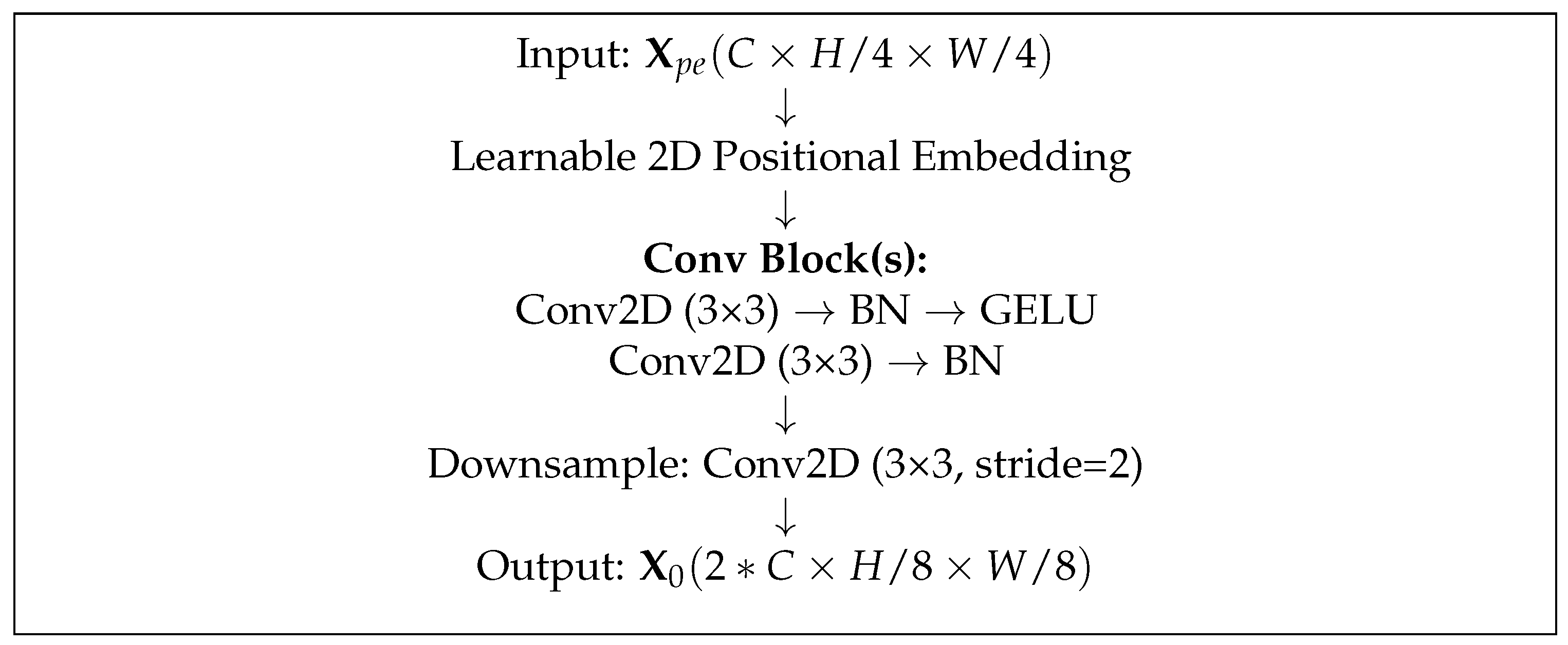
The module (Figure 1) contains two sequential $3\times 3$ convolutional layers with stride 2, which are separated by batch normalization and ReLU activation layers. The output of this process results in a feature map that has been reduced by a factor of 4. A learnable 2D positional embedding $\mathbf{P}\in {\mathbb{R}}^{1\times C\times H/4\times W^{\prime }/4}$ is added to the result to maintain spatial awareness that was lost during downsampling:

$${\mathbf{X}}_{pe}={\mathtt{Conv}}_{\mathrm{stride}=2}^{\left(2\right)}\left(\mathbf{X}\right)+{\mathbf{P}}_{\mathbf{1}}.$$

The output of this patch embedding module becomes the low-resolution feature grid, which serves as the input to the hierarchical encoder stages.

3.3. Stage 1: Positional-Aware Convolutional Stem

The first stage of UltraScanNet functions as a spatially grounded stem block that extracts low-level features while maintaining the positional structure of the input image.

The module (Figure 2) consists of two consecutive $3\times 3$ convolutional layers with stride 1, followed by batch normalization (both) and GELU activation (just the first convolution). The spatial resolution decreases further by a factor of $2\times$, while the feature dimensionality increases through this process.

The module also benefits from spatial layout awareness through learnable 2D positional embeddings ${\mathbf{P}}_{\mathbf{2}}\in {\mathbb{R}}^{1\times C\times H/4\times W/4}$, which are added just before the convolutional stack:

$${\mathbf{X}}_0={\mathrm{ConvBNGELU}}_2\left({\mathrm{ConvBN}}_1\left({\mathbf{X}}_{\mathbf{pe}}\right)\right)+{\mathbf{P}}_{\mathbf{2}}.$$

The spatial dimensions after downsampling are represented by $H/8$ and $W/8$, while C represents the feature dimension.

3.4. Stage 2: Hybrid Local–Global Encoding

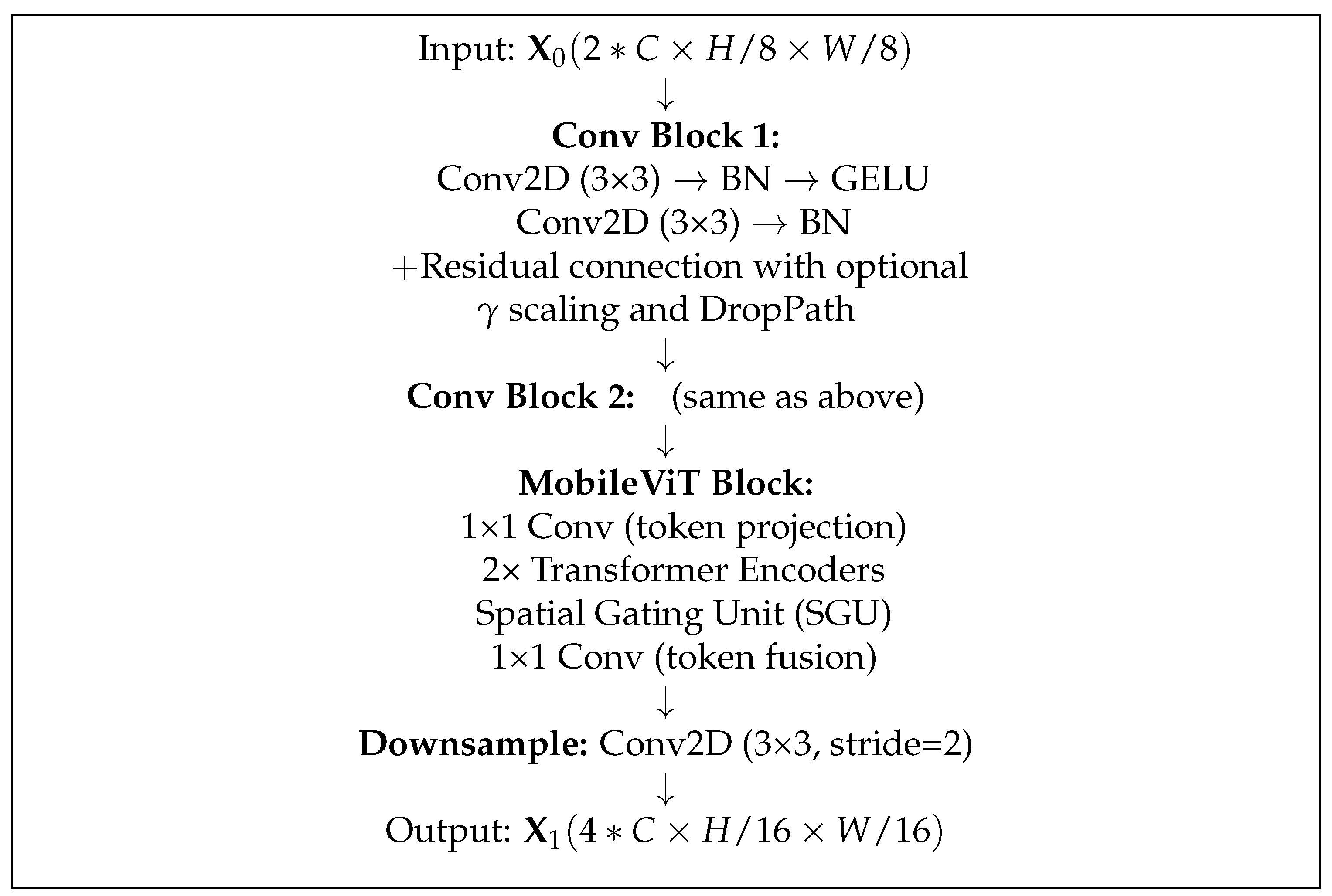
The initial encoding block of UltraScanNet (Figure 3) combines spatial pattern detection with short-range contextual information processing in its first stage. The encoding process uses two sequential convolutional blocks with a lightweight Transformer-inspired module that combines MobileViT and spatial gating.

Local Feature Encoding. The initial stage consists of two standard convolutional residual blocks that use $3\times 3$ convolutions, followed by batch normalization and GELU [47] nonlinear activation. The blocks detect localized features including edges, contours, and lesions, which are prominent in breast ultrasound images.

Global Token Mixing. The MobileViT architecture serves as the foundation for our lightweight token mixer to enhance the convolutional spatial locality. Specifically, we integrate

• A $1\times 1$ convolution that serves as the token projection operation;
• Two stacked Transformer encoder layers that perform multi-head self-attention on reshaped $N\times C$ token sequences;
• The spatial gating unit (SGU), which learns a gating mask to modulate each spatial location;
• A fusion layer that transforms tokens into spatial feature maps.

The combined approach enables the model to generate representations that describe both local details and global coherence, which suits ultrasound imaging because the anatomical context is important despite limited annotation.

Downsampling. The hybrid block follows a $3\times 3$ strided convolution that decreases the spatial dimensions and increases the feature dimensions for deeper processing.

$${\mathbf{X}}_1=\mathtt{Downsample}\left(\mathtt{MobileViT}\left({\mathtt{Conv}}_2\left({\mathtt{Conv}}_1\left({\mathbf{X}}_0\right)\right)\right)\right).$$

The output ${\mathbf{X}}_1$ maintains local details while incorporating self-attended contextual information.

3.5. Stage 3: Progressive Global Context Modeling

The concluding components in the UltraScanNet system enable the efficient handling of spatial and temporal dependencies of variable scope. A sequence of depth-adaptive blocks exists in each stage of the network, which determines the mixing operation based on its stage depth index.

The block index i dictates which operation to apply to each stage according to the following rules:

• The proposed UltraScanUnit represents the selective scan mechanism with state-space inspiration that uses convolutional residuals together with low-rank projection for early blocks ($i<d/2$);
• The ConvAttnMixer block operates at the middle of the stage ($i=d/2$) to merge spatial information with channel-based mixing;
• The last blocks of the sequence ($i>d/2$) use multi-head self-attention (MHSA) for global feature refinement.

The depth-based scheduling system allows the model to start with a selective scan for mid-range dependency encoding before moving to spatial channel mixing and ending with global attention.

3.5.1. UltraScanUnit: Temporally Aware State-Space Module with Convolutional Residuals

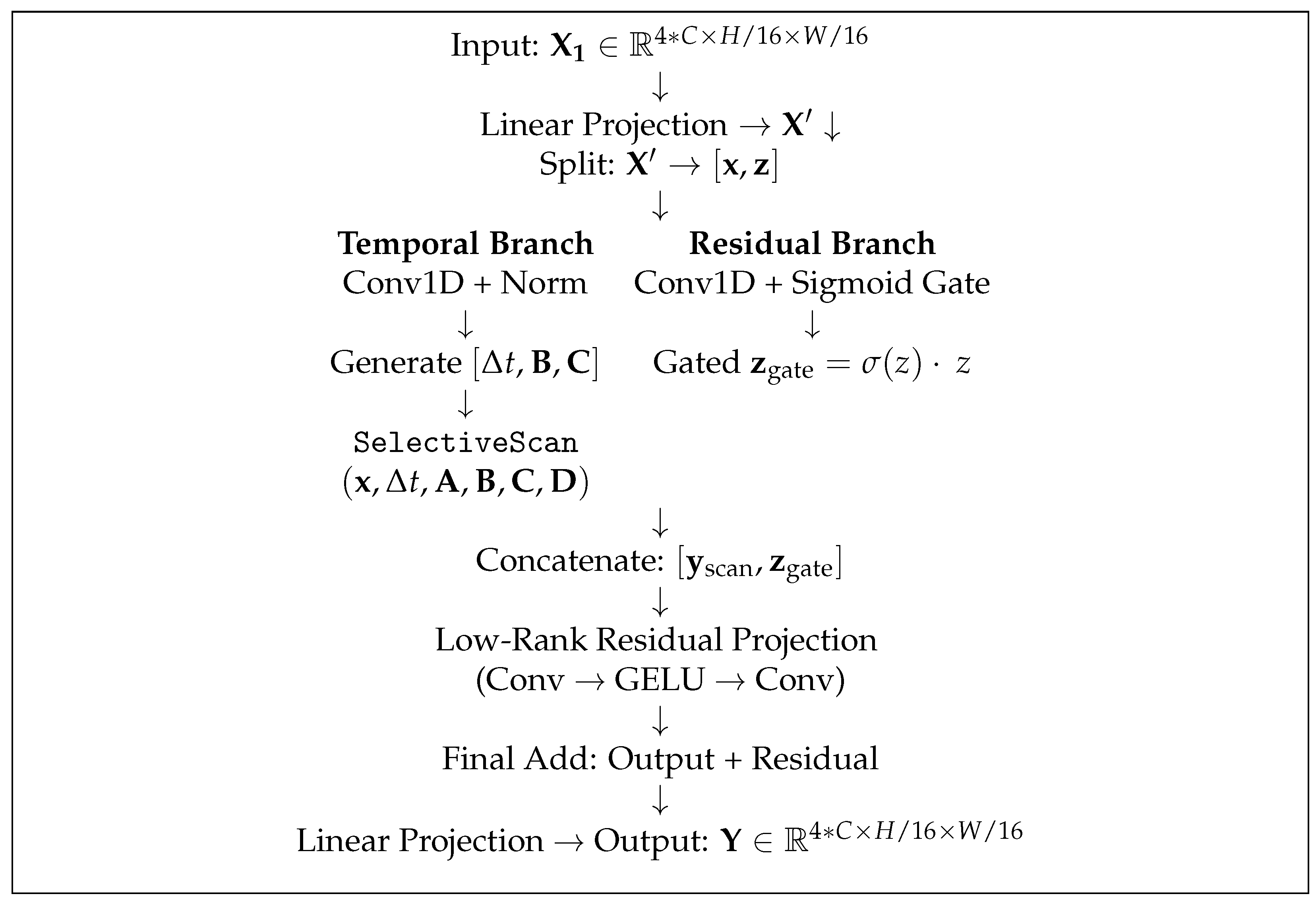
The proposed UltraScanUnit module (Figure 4) draws inspiration from the Mamba architecture [24] and specifically from the MambaVision network [25], but it is specifically designed for processing grayscale breast ultrasound images. It uses state-space sequence modeling together with convolutional priors and gated residual connections to encode temporal dependencies efficiently while maintaining gradient stability.

Input Projection

The input tensor ${\mathbf{X}}_{\mathbf{1}}$ with dimensions $4\ast C\times H/16\times W/16$ undergoes a linear transformation that maintains the feature count.

Temporal Modeling via Selective Scan

The output of the $\mathbf{x}$ stream goes through a feedforward layer that generates dynamic parameters $\Delta t,\mathbf{B},\mathbf{C}$. The model combines the global decay weights $\mathbf{A}$ with the skip weights $\mathbf{D}$ and the calculated $\Delta t$ to perform the selective scan. The output of the SelectiveScan operation becomes ${\mathbf{y}}_{\mathrm{scan}}$ when it processes the input $\mathbf{x}$ with $\Delta t$ and weights $\mathbf{A}$, $\mathbf{B}$, $\mathbf{C}$, and $\mathbf{D}$.

Gated Residual Branch

The $\mathbf{z}$ stream passes through convolutional and gating operations. The result of applying Conv1D to $\mathbf{z}$ goes through the GELU activation function before obtaining ${\mathbf{z}}_{\mathrm{gate}}=\sigma \left(\mathtt{Conv}\mathtt{1}\mathtt{D}\left(\mathbf{z}\right)\right)\odot \mathbf{z}$. The final output is the result of combining the scan output with the gated output.

$${\mathbf{y}}_{\mathrm{cat}}=[{\mathbf{y}}_{\mathrm{scan}},{\mathbf{z}}_{\mathrm{gate}}].$$

A parallel low-rank residual path operates on the concatenated input. The output of the Conv1D operation, followed by GELU and another Conv1D operation on the input $[\mathbf{x},\mathbf{z}]$, produces $\mathbf{r}$. The output of the final operation becomes ${\mathbf{y}}_{\mathrm{final}}={\mathbf{y}}_{\mathrm{cat}}+\mathbf{r}$.

Final Projection

The output is rearranged through projection into its original dimensions. The output tensor $\mathbf{Y}$ results from applying a linear transformation to the output of $\mathtt{Rearrange}({\mathbf{y}}_{\mathrm{final}}$), which has the same dimensions as the input feature map: $4\ast C\times H/16\times W/16$.

The hybrid approach within UltraScanUnit allows it to effectively detect both local and distant signal relationships through an efficient computational framework that suits the spatiotemporal characteristics of the ultrasound signal.

3.5.2. ConvAttnMixer

A ConvAttnMixer block serves as the bridge to unite convolutional processing with attention mechanisms through the following components:

• The depthwise separable convolution operates with a $k\times k$ filter to maintain spatial bias;
• Token normalization is performed through LayerNorm;
• The feedforward module performs point-wise operations to enhance cross-channel interactions.

3.5.3. Attention Blocks

The later blocks of the network employ MHSA with scaled dot-product attention, which produces outputs that are projected and then passed through dropout. These blocks refine the feature representations globally and benefit from the reduced spatial resolution obtained in prior stages. We keep these blocks as in [25], having the same attention heads as well.

Windowed Processing. Attention memory usage decreases through the implementation of window partitioning with fixed dimensions w across both the vertical and horizontal axes. The process includes padding for cases when the input dimensions are not multiples of w.

$${\mathbf{X}}_{\mathrm{out}}={\mathtt{Block}}_d\circ \cdots \circ {\mathtt{Block}}_1\left(\mathtt{WindowPartition}\left(X\right)\right).$$

3.5.4. Downsampling and Final Prediction

The feature map undergoes an optional downsampling operation through strided convolution in the first Stage 3 layer. The spatial resolution of the second and last Stage 3 layers remains intact, while it functions as an elevated context processor before moving to global pooling. Therefore, the last feature map dimension is equal to $8\ast C\times H/32\times W/32$.

Finally, channel-wise normalization, global average pooling, and a linear classifier produce three logits (benign, malignant, normal), with softmax yielding class probabilities.

Putting it all together, the UltraScanNet architecture can be seen in Figure 5.

4. Experimental Setup

4.1. Datasets

The evaluation of UltraScanNet is performed on BUSI [18], which is a public breast ultrasound dataset that contains 780 grayscale images that are labeled as benign, malignant, or normal. The BUSI dataset’s images naturally contain varying levels of speckle noise; therefore, the proposed method and the evaluation results inherently consider the model’s robustness to this.

In addition to this, we conducted a cross-dataset evaluation on the BUS-UCLM dataset [48], which contains ultrasound images acquired using different devices and protocols, enabling an assessment of the model’s generalization capabilities across domains.

All images are stored as 3-channel PNGs, and, before being fed to the model, they are resized to $224\times 224$ and normalized. Because there is no available information about which image corresponds to which patient, we cannot enforce a patient-level split and instead use an 80/20 stratified train/validation split for each setting.

4.2. Data Augmentation and Preprocessing

We use moderate data augmentation to enhance the robustness of the models due to the limited size of the dataset:

• Random horizontal flip with probability 0.5;
• Color jitter with intensity 0.2—the value of 0.2 was chosen after running an experiment series with jitter values from 0.0 to 0.5;
• AutoAugment: a RandAugment policy with magnitude 9 and standard deviation 0.5;
• Mixup and CutMix with $\alpha =0.2$ and switch probability 0.5;
• Random resized crops with an area scale sampled from [0.08, 1.0] and a ratio from [0.75, 1.33];
• Bicubic interpolation for resizing.

The images are converted to channels-last format, and they are optionally padded to a square shape. We use class label smoothing of $ϵ=0.1$ during training to prevent overfitting.

4.3. Training Configuration

The optimizer used is AdamW with ${\beta }_1=0.9$, ${\beta }_2=0.999$, $ϵ={10}^{-8}$ and weight decay of $0.01$. The learning rate is set to $6.25\times {10}^{-5}$ and decays following a cosine annealing schedule. We apply a linear warmup for the first 20 epochs, starting at $6.25\times {10}^{-8}$. The learning rate reaches a minimum of $6.25\times {10}^{-7}$. Other training details are as follows:

• Epochs: 150 total (with early stopping patience of 10 epochs);
• Batch size: 32 for training, 16 for validation;
• Gradient clipping: norm-based with a maximum of 5.0;
• DropPath rate: 0.2 across the model;
• Mixed precision: enabled using PyTorch 2.7.0 AMP.

We train the models on a single NVIDIA GeForce RTX 4070 Ti GPU with 8 workers for data loading.

4.4. Pretraining and Initialization

Standard baseline models (e.g., MambaVision [25], ResNet [21], ViT [23], Swin [32], ConvNeXt [28]) were initialized with pretrained weights from the ImageNet-1K classification task. For UltraScanNet, we partially reused pretrained weights from the original MambaVision-Tiny [25] model. Specifically, components that remained unchanged from the base architecture (e.g., the attention module) were initialized from ImageNet-1K [49], while newly introduced modules such as UltraScanUnit, the hybrid Stage 1, or the convolutional attention blocks from the middle of Stages 2 and 3 were randomly initialized using standard initialization techniques.

5. Results

The evaluation of our proposed UltraScanNet model takes place through testing on the BUSI dataset for breast ultrasound image classification. The evaluation of our model includes comparisons with multiple state-of-the-art convolutional neural networks (CNNs), Transformer-based architectures, and Mamba-based models. The evaluation process uses identical training and evaluation protocols to ensure fair model comparisons.

5.1. Macro Accuracy, Precision, Recall, and F1-Score

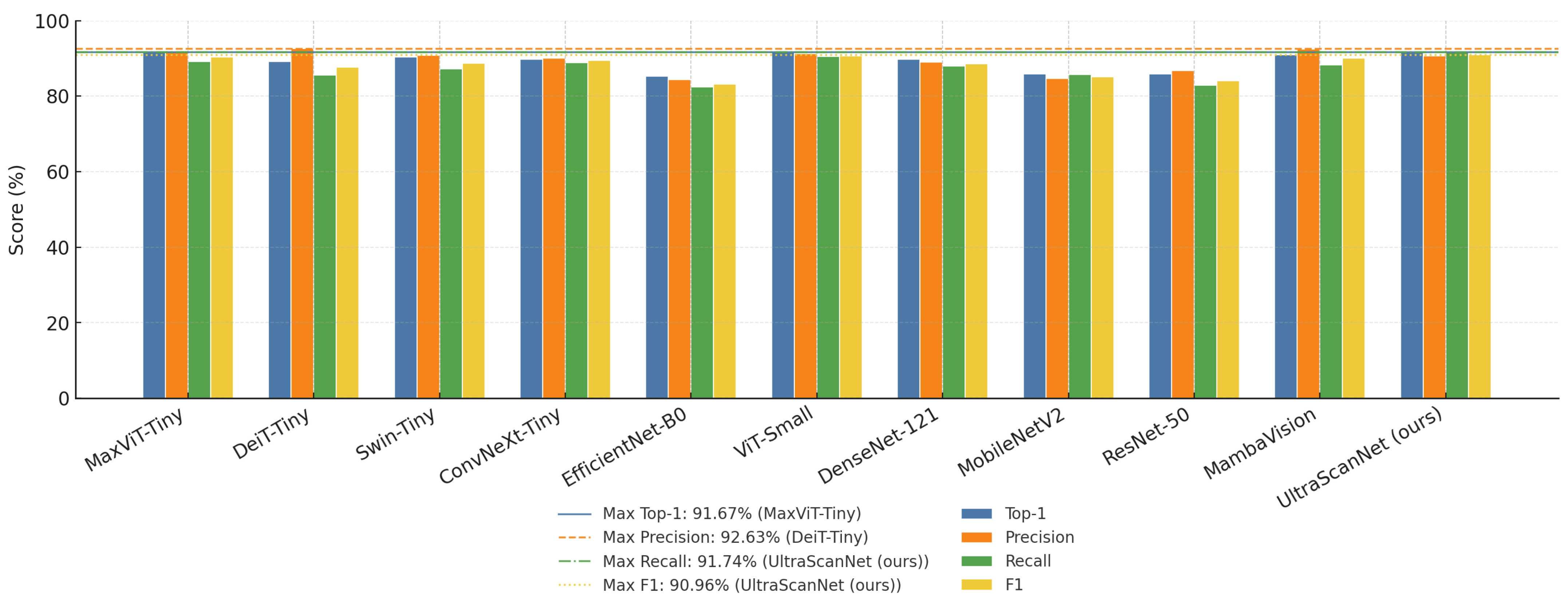
The BUSI dataset receives the first evaluation, illustrated in

Table 1. Model performance on the BUSI dataset. Best value in each column is in bold.

Model	Loss	Top-1 Accuracy (%)	Precision	Recall	F1-Score
MaxViT-Tiny [50]	0.3465	91.67	0.9187	0.8915	0.9040
DeiT-Tiny [31]	0.4057	89.10	0.9263	0.8563	0.8764
Swin-Tiny [32]	0.3528	90.38	0.9074	0.8715	0.8864
ConvNeXt-Tiny [28]	0.3406	89.74	0.9000	0.8885	0.8941
EfficientNet-B0 [51]	0.4703	85.26	0.8439	0.8242	0.8314
ViT-Small [23]	0.3203	91.67	0.9120	0.9044	0.9073
DenseNet-121 [27]	0.3882	89.74	0.8906	0.8803	0.8850
MobileNetV2 [52]	0.4674	85.90	0.8460	0.8576	0.8514
ResNet-50 [21]	0.5047	85.90	0.8680	0.8286	0.8400
MambaVision [25]	0.3505	91.02	0.9241	0.8832	0.9003
UltraScanNet (ours)	0.3367	91.67	0.9072	0.9174	0.9096

, which shows the top-1 classification accuracy, precision, recall, and F1-score results for each model. The values can also be visualized as grouped charts in Figure 6.

UltraScanNet achieves top-1 accuracy of 91.67%, which equals the accuracy of MaxViT-Tiny [50] and ViT-Small [23]. On top of this, the proposed model renders better results than all other evaluated models in terms of recall (0.9174) and the F1-score (0.9096), which is a crucial requirement for medical diagnostics because false negatives are particularly critical.

Our model achieves a significant accuracy improvement of +1.93% and +5.77% compared to the CNN-based backbones, including ConvNeXt-Tiny [28] (89.74%) and ResNet-50 (85.90%). The model outperforms MobileNetV2 [52] and EfficientNet-B0 [51] by +5.77% and +6.41%, respectively, while maintaining a competitive loss value of 0.3367.

UltraScanNet demonstrates better performance compared to the DeiT-Tiny [31] and Swin-Tiny [32] Transformer-based models, which were designed for data efficiency and hierarchical attention. The combination of state-space modeling through UltraScanUnit with spatial gating in a hybrid architecture proves effective for low-data grayscale medical applications.

The high recall and F1-score of UltraScanNet indicate its suitability for clinical use because it minimizes false negatives, which have serious implications in medical practice. The obtained results confirm our design decisions and demonstrate how the model combines local feature extraction with global context reasoning and efficient temporal modeling.

5.2. Comparison with MambaVision

Table 2. Mean accuracy and standard deviation comparison between UltraScanNet and MambaVision.

Model	Mean Accuracy (%)	Std. Dev. (%)
UltraScanNet (ours)	91.03	±0.80
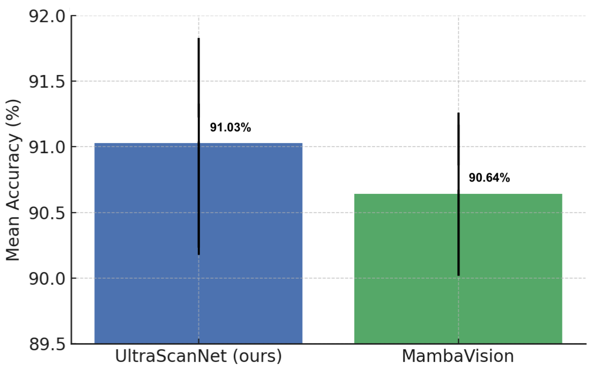
MambaVision	90.64	±0.62

and Figure 7 present the mean accuracy and standard deviation across multiple runs for UltraScanNet and the MambaVision [25] model.

Table 2 and Figure 7 illustrate that UltraScanNet achieves +0.39% higher mean accuracy than MambaVision [25]. The standard deviation is slightly higher for UltraScanNet (+0.18%), indicating a small trade-off in stability. Even so, in practical terms, UltraScanNet consistently performs better than the baseline in terms of average accuracy while maintaining variance at a reasonable level.

5.3. Per-Class Precision, Recall, and F1-Score

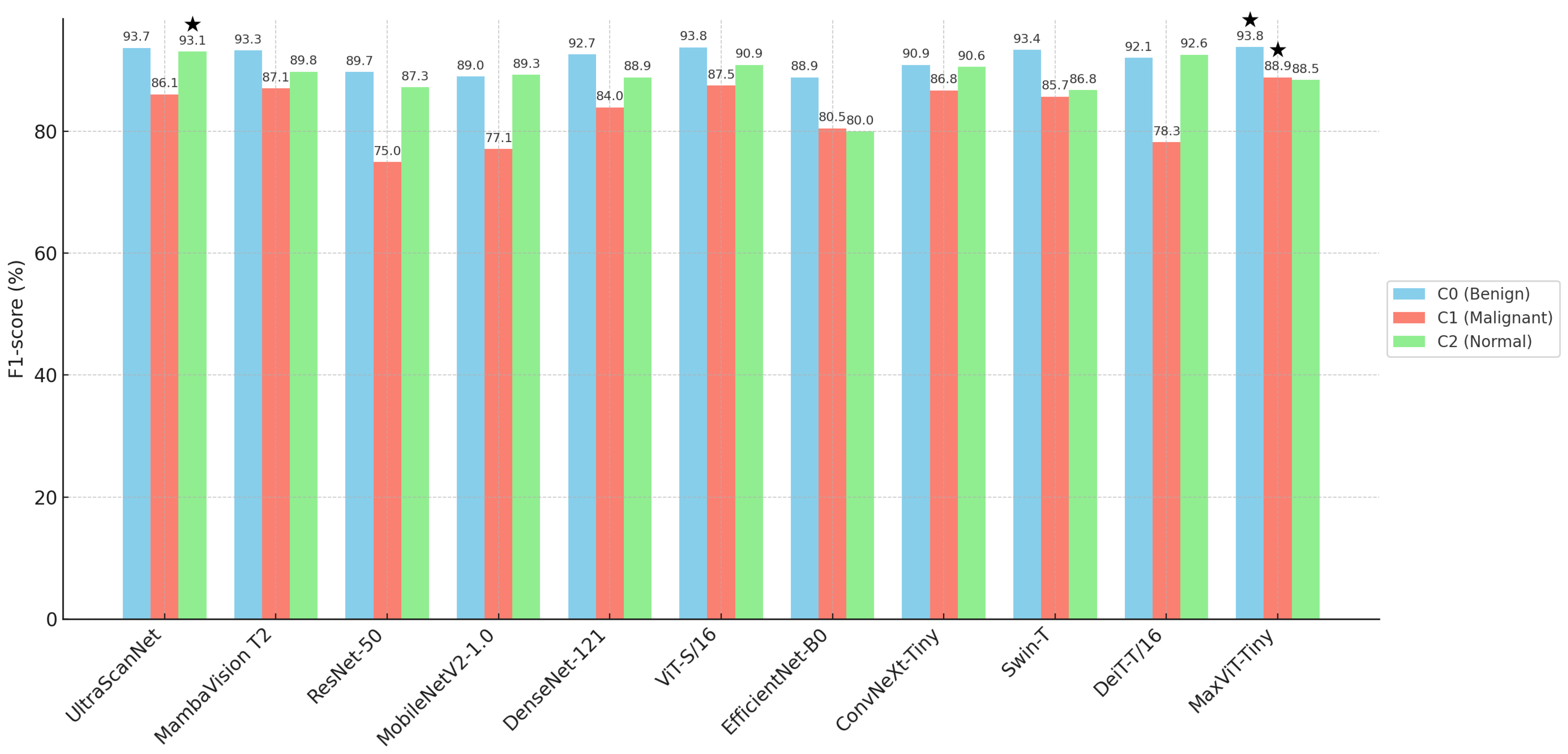
The performance metrics in

Table 3. Per-class performance on BUSI. Classes: C0 = benign, C1 = malignant, C2 = normal. Best value in each column is in bold.

Model	Precision (%)			Recall (%)			F1 (%)
	C0	C1	C2	C0	C1	C2	C0	C1	C2
UltraScanNet (ours)	93.18	91.89	87.10	94.25	80.95	100.00	93.71	86.08	93.10
MambaVision T2 (baseline)	91.21	86.05	100.00	95.40	88.10	81.48	93.26	87.06	89.80
ResNet-50	84.69	90.00	85.71	95.40	64.29	88.89	89.73	75.00	87.27
MobileNetV2-1.0	89.53	78.05	86.21	88.51	76.19	92.59	89.02	77.11	89.29
DenseNet-121	91.11	87.18	88.89	94.25	80.95	88.89	92.66	83.95	88.89
ViT-S/16	92.22	92.11	89.29	95.40	83.33	92.59	93.79	87.50	90.91
EfficientNet-B0	86.02	88.57	78.57	91.95	73.81	81.48	88.89	80.52	80.00
ConvNeXt-Tiny	89.89	87.80	92.31	91.95	85.71	88.89	90.91	86.75	90.57
Swin-T (patch4, window7)	89.47	94.29	88.46	97.70	78.57	85.19	93.41	85.71	86.79
DeiT-T/16	85.29	100.00	92.59	100.00	64.29	92.59	92.06	78.26	92.59
MaxViT-Tiny	91.30	92.31	92.00	96.55	85.71	85.19	93.85	88.89	88.46

and the grouped bar charts in Figure 8 demonstrate that UltraScanNet maintains a balanced performance profile. The model achieves the highest recall and F1-score for the normal class (C2) and achieves the highest precision for the benign class (C0). The model’s performance suggests that it can minimize unnecessary alarms and patient distress by showing fewer normal cases as lesions. Moreover, the model achieves this performance level by maintaining high accuracy in benign case detection at the same time.

Models like DeiT-T/16 (perfect precision on C1) and MambaVision T2 (perfect precision on C2, highest malignant recall) exhibit specialized strengths, useful depending on whether clinical priorities favor minimizing false positives or false negatives.

The radar plots in Figure 9 provide an overview of how each class performs in each model. UltraScanNet demonstrates consistent performance across all three classes and achieves its best results on the normal class (C2). The precision of DeiT-T/16 reaches its peak at perfect levels when detecting the malignant class (C1), while MambaVision achieves high recall rates for the same class. The precision and recall of MaxViT-Tiny and ViT-S/16 also show competitive values.

The radar plots show that UltraScanNet maintains equal performance in terms of precision, recall, and the F1-score across all classes, while other architectures tend to excel in one metric or one class at the expense of others.

5.4. Per-Class ROC–AUC and PR–AUC

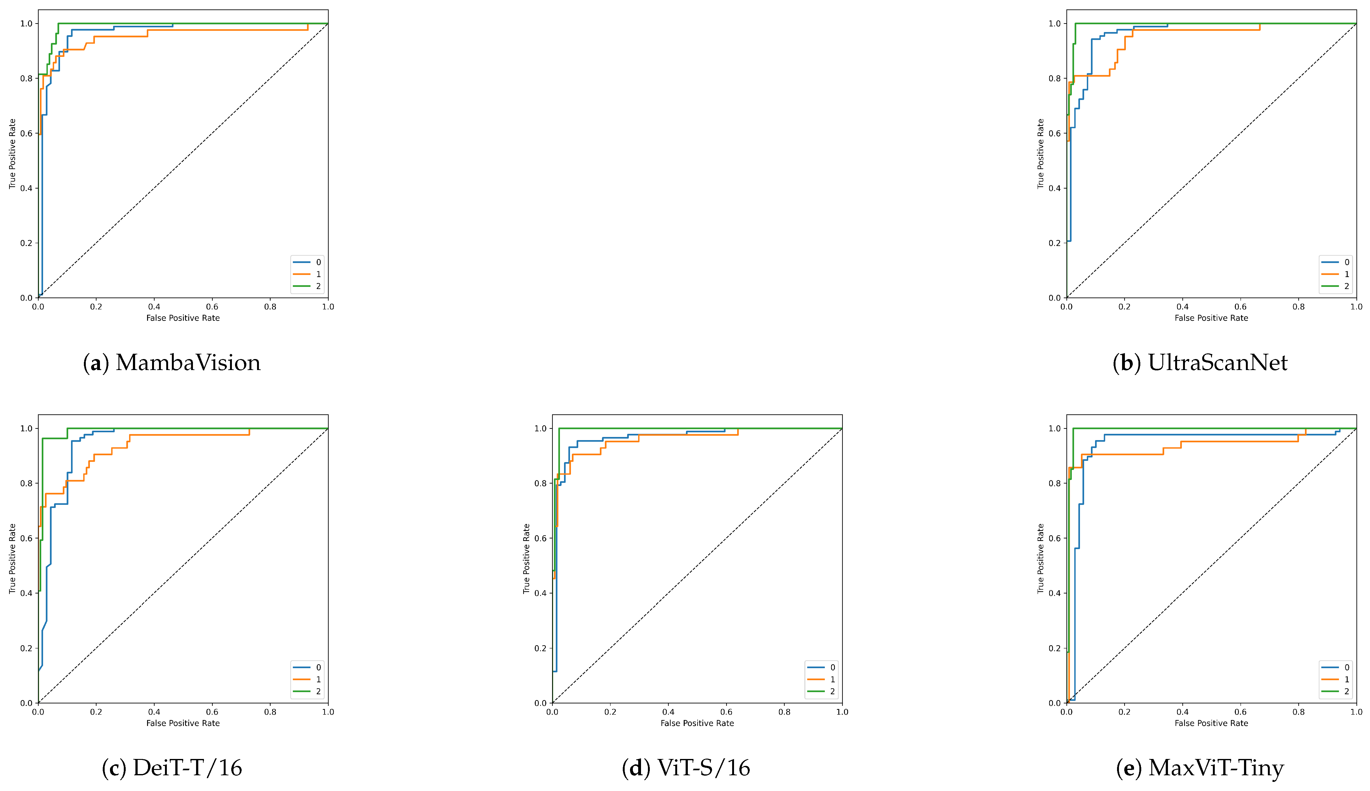
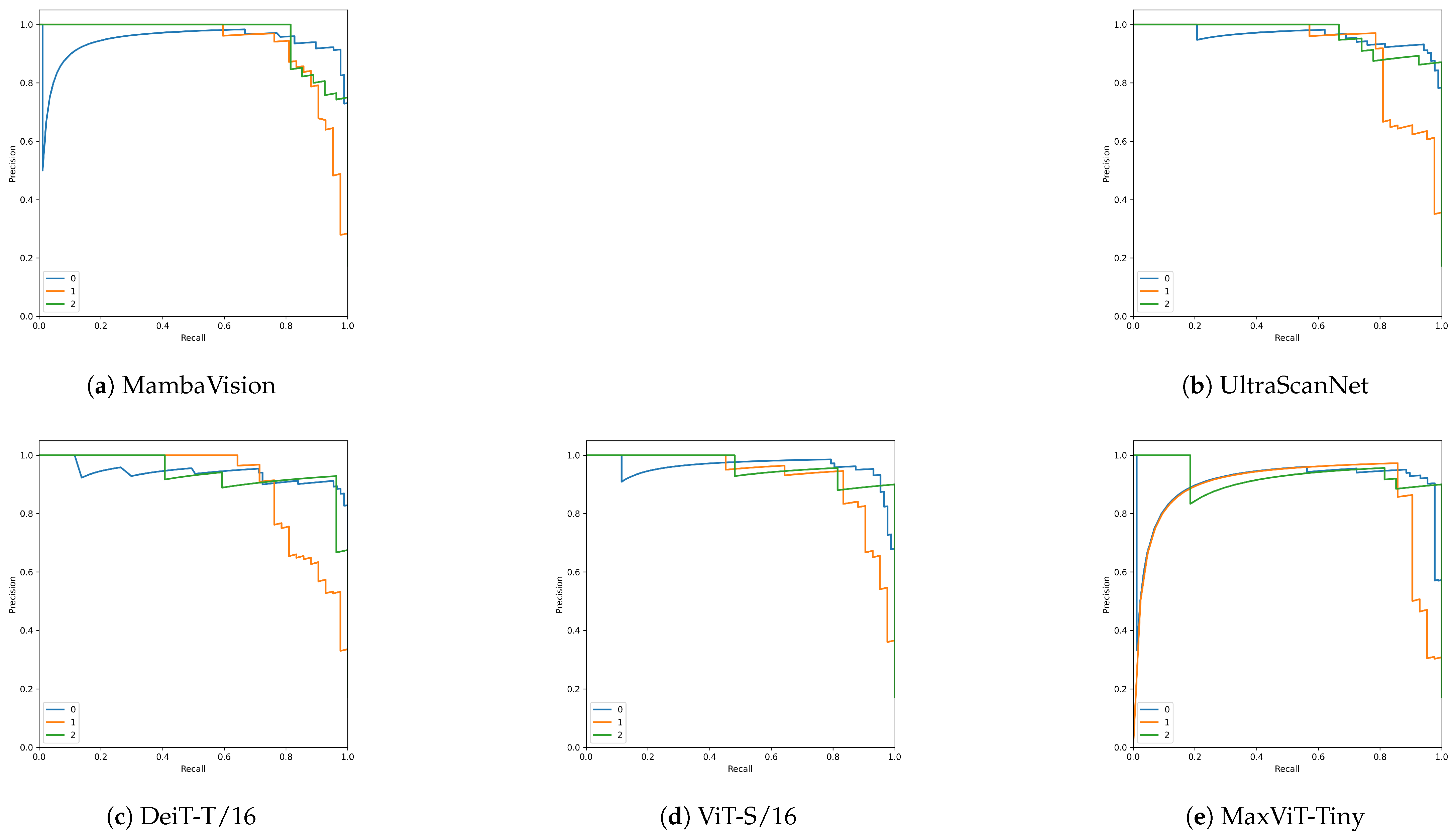
The ROC–AUC and PR–AUC values per class in

Table 4. Per-class ROC–AUC and PR–AUC on BUSI (%). Classes: C0 = benign, C1 = malignant, C2 = normal. Best value in each column is in bold.

Model	ROC–AUC			PR–AUC
	C0	C1	C2	C0	C1	C2
UltraScanNet (ours)	96.19	95.07	99.31	96.08	91.55	96.60
MambaVision	96.33	95.23	99.08	93.93	93.07	96.24
ResNet-50	94.02	94.70	96.63	95.68	88.39	83.39
MobileNetV2-1.0	93.49	92.44	98.19	94.47	86.67	93.78
DenseNet-121	96.92	96.35	98.32	97.54	91.75	95.10
ViT-S/16	96.44	95.97	99.31	96.10	92.63	96.13
EfficientNet-B0	91.21	91.83	97.16	92.29	83.08	87.18
ConvNeXt-Tiny	94.44	93.98	98.88	91.68	92.89	92.70
Swin-T (patch4, window7)	93.29	89.81	98.22	90.97	89.33	94.58
DeiT-T/16	94.79	93.90	98.91	93.92	89.97	94.22
MaxViT-Tiny	93.70	93.40	99.11	90.06	84.80	96.60

and Figure 10 and Figure 11 demonstrate the ranking quality and precision–recall trade-offs for each model.

The ROC–AUC values of DenseNet-121 demonstrate the best separation between the benign (C0) and malignant (C1) classes with 96.92% and 96.35%, respectively. The top score of 99.31% for normal (C2) classification belongs to both UltraScanNet and ViT-S/16 because they achieve the near-perfect discrimination of normal tissue.

The PR–AUC results show that DenseNet-121 leads in C0 (97.54%), MambaVision leads in C1 (93.07%), and UltraScanNet and MaxViT-Tiny tie for C2 (96.60%). The high PR–AUC value in C1 is especially important in clinical scenarios with class imbalance because it demonstrates the model’s ability to preserve its precision when malignant cases appear infrequently.

The ROC–AUC results show that DenseNet-121 performs best in most classes, but UltraScanNet matches or outperforms it in C2 discrimination and maintains an overall competitive PR–AUC profile. The results demonstrate that UltraScanNet performs well in distinguishing normal tissue, while maintaining good performance across different lesion types.

Figure 12 and Figure 13 compare the precision–recall trade-offs across classes for MambaVision and UltraScanNet. While the baseline model exhibits sharper variations in recall for malignant cases (C1), UltraScanNet demonstrates overall smoother curves and better recall preservation at higher thresholds, especially in normal class (C2). This suggests that UltraScanNet can operate more reliably across different decision thresholds, an important property for clinical deployment.

5.5. Sensitivity @ 90% Specificity

The next evaluation of the models (

Table 5. Sensitivity at 90% specificity for each class on BUSI (%). Classes: C0 = benign, C1 = malignant, C2 = normal. Best value in each column is in bold.

Model	C0	C1	C2
UltraScanNet (ours)	81.61	80.95	92.59
MambaVision T2 (baseline)	89.66	88.10	96.30
ResNet-50	80.46	80.95	88.89
MobileNetV2-1.0	72.41	73.81	92.59
DenseNet-121	86.21	80.95	92.59
ViT-S/16	93.10	88.10	81.48
EfficientNet-B0	73.56	73.81	85.19
ConvNeXt-Tiny	89.66	90.48	96.30
Swin-T (patch4, window7)	82.76	80.95	92.59
DeiT-T/16	72.41	78.57	96.30
MaxViT-Tiny	93.10	85.71	85.19

) considers a fixed high specificity value (90%) and assesses their sensitivity performance under strict false-positive control conditions, which are crucial for breast cancer screening.

As can be seen, the ViT-S/16 and MaxViT-Tiny models demonstrate the highest sensitivity (93.10%) in detecting benign lesions (C0), while maintaining low false alarm rates. On the other hand, ConvNeXt-Tiny demonstrates the highest sensitivity of 90.48% for malignant (C1) cases, while maintaining the lowest false-positive rate. Finally, the three models MambaVision T2, ConvNeXt-Tiny, and DeiT-T/16 achieve the highest sensitivity of 96.30% for normal (C2) cases, which indicates that they rarely miss normal cases at high specificity levels.

These results demonstrate that UltraScanNet maintains competitive values across all classes, yet certain models achieve better performance in specific classes under constrained sensitivity conditions. The deployment of these models depends on the primary objective, i.e., whether it is to detect malignant lesions, maintain benign specificity, or avoid normal cases’ misclassification.

5.6. F1-Macro Mean and 95% Confidence Intervals

Table 6. F1-macro mean and 95% confidence intervals on BUSI. Classes: C0 = benign, C1 = malignant, C2 = normal. Best value in each column is in bold.

Model	F1-Macro Mean	95% CI Low	95% CI High
UltraScanNet (ours)	0.909	0.860	0.953
MambaVision T2 (baseline)	0.899	0.841	0.949
ResNet-50	0.837	0.773	0.899
MobileNetV2-1.0	0.851	0.787	0.909
DenseNet-121	0.882	0.823	0.939
ViT-S/16	0.905	0.850	0.955
EfficientNet-B0	0.830	0.762	0.890
ConvNeXt-Tiny	0.893	0.838	0.941
Swin-T (patch4, window7)	0.885	0.822	0.939
DeiT-T/16	0.874	0.812	0.928
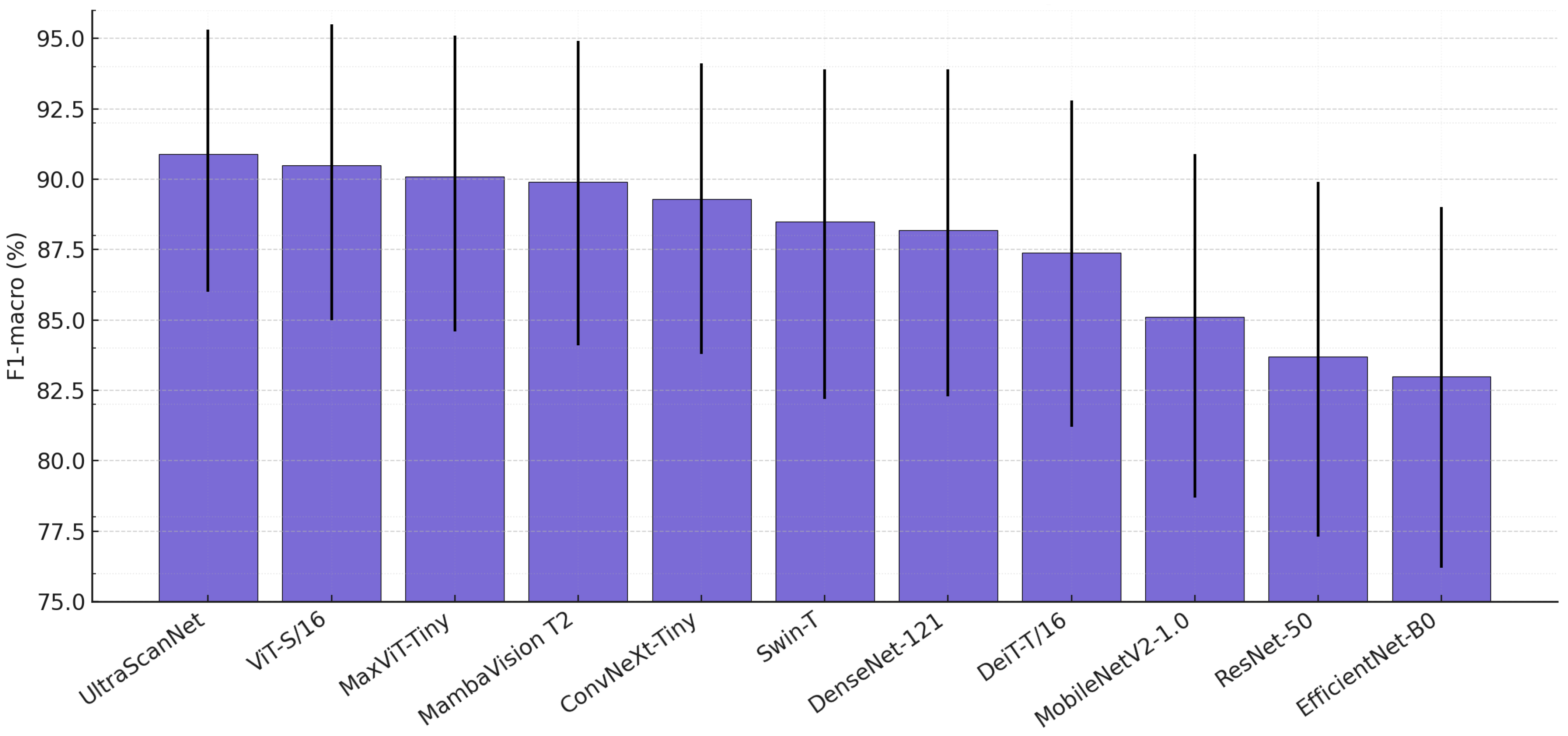
MaxViT-Tiny	0.901	0.846	0.951

and Figure 14 present the macro-averaged F1-scores together with their 95% confidence intervals, which show both the estimated values and their corresponding uncertainty intervals.

UltraScanNet demonstrates the highest F1-macro mean value of 0.909 because it maintains balanced performance across all classes.

The 95% CI lower bound reaches its highest value at 0.846 with MaxViT-Tiny, indicating that this model performs well even in the most unfavorable sampling conditions. The upper bound of ViT-S/16 reaches 0.955, which indicates that its peak performance might match or surpass that of UltraScanNet under optimal circumstances.

These results show that UltraScanNet demonstrates the best overall balance, but MaxViT-Tiny provides the most reliable lower-bound results, and ViT-S/16 demonstrates the highest potential maximum performance.

5.7. Recall and AUC with 95% Confidence Intervals

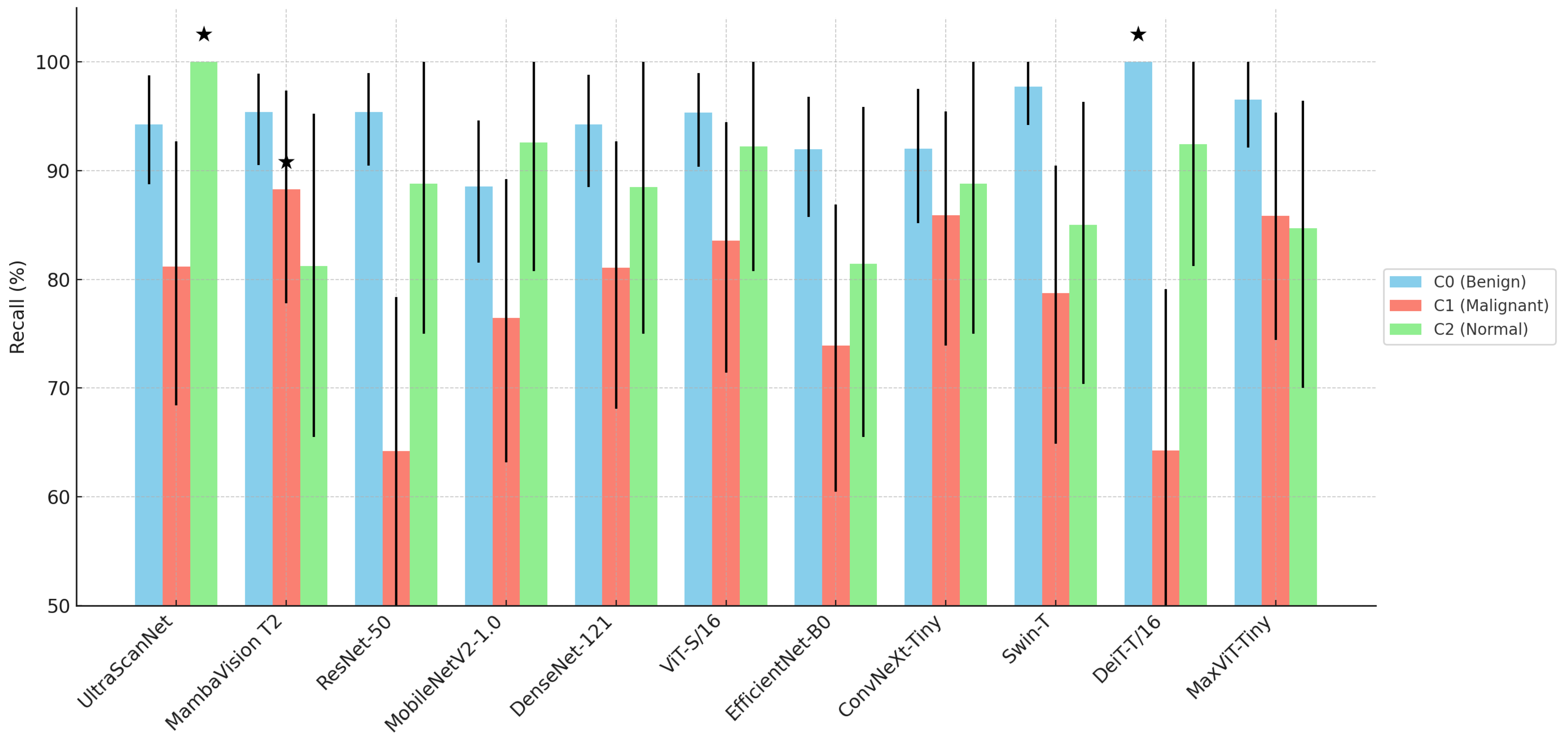
The recall CIs in

Table 7. Per-class recall mean and 95% confidence intervals on BUSI. Classes: C0 = benign, C1 = malignant, C2 = normal. Best value in each column is in bold.

Model	Recall Mean			95% CI Low			95% CI High
	C0	C1	C2	C0	C1	C2	C0	C1	C2
UltraScanNet (ours)	94.25	81.16	100.00	88.76	68.42	100.00	98.78	92.68	100.00
MambaVision T2 (baseline)	95.41	88.30	81.22	90.53	77.78	65.51	98.91	97.37	95.24
ResNet-50	95.39	64.20	88.79	90.47	48.89	75.00	98.94	78.38	100.00
MobileNetV2-1.0	88.55	76.46	92.57	81.52	63.15	80.77	94.63	89.19	100.00
DenseNet-121	94.25	81.07	88.48	88.46	68.08	75.00	98.80	92.68	100.00
ViT-S/16	95.33	83.54	92.23	90.36	71.42	80.77	98.97	94.44	100.00
EfficientNet-B0	91.97	73.90	81.43	85.71	60.45	65.52	96.77	86.85	95.84
ConvNeXt-Tiny	92.01	85.88	88.78	85.18	73.91	75.00	97.50	95.45	100.00
Swin-T (patch4, window7)	97.70	78.72	84.99	94.18	64.86	70.37	100.00	90.48	96.30
DeiT-T/16	100.00	64.24	92.45	100.00	48.83	81.24	100.00	79.07	100.00
MaxViT-Tiny	96.55	85.85	84.68	92.13	74.42	70.00	100.00	95.35	96.43

and in Figure 15 reflect each model’s ability to consistently identify cases within each class across repeated sampling.

• Benign (C0): DeiT-T/16 attains a perfect recall mean (100%) with a narrow CI, ensuring that benign lesions are consistently detected. Swin-T also performs exceptionally (97.70%), showing high reliability in this class.
• Malignant (C1): MambaVision T2 reaches the highest recall mean (88.30%), indicating strong sensitivity to malignant cases. ConvNeXt-Tiny has the highest lower bound (73.91%), suggesting more stable performance under resampling.
• Normal (C2): UltraScanNet is the only model that achieves perfect recall (100%) in the evaluated folds, which means that it never misclassifies normal cases. Several other models match this in the upper bound but not in the mean, underscoring UltraScanNet’s robustness.

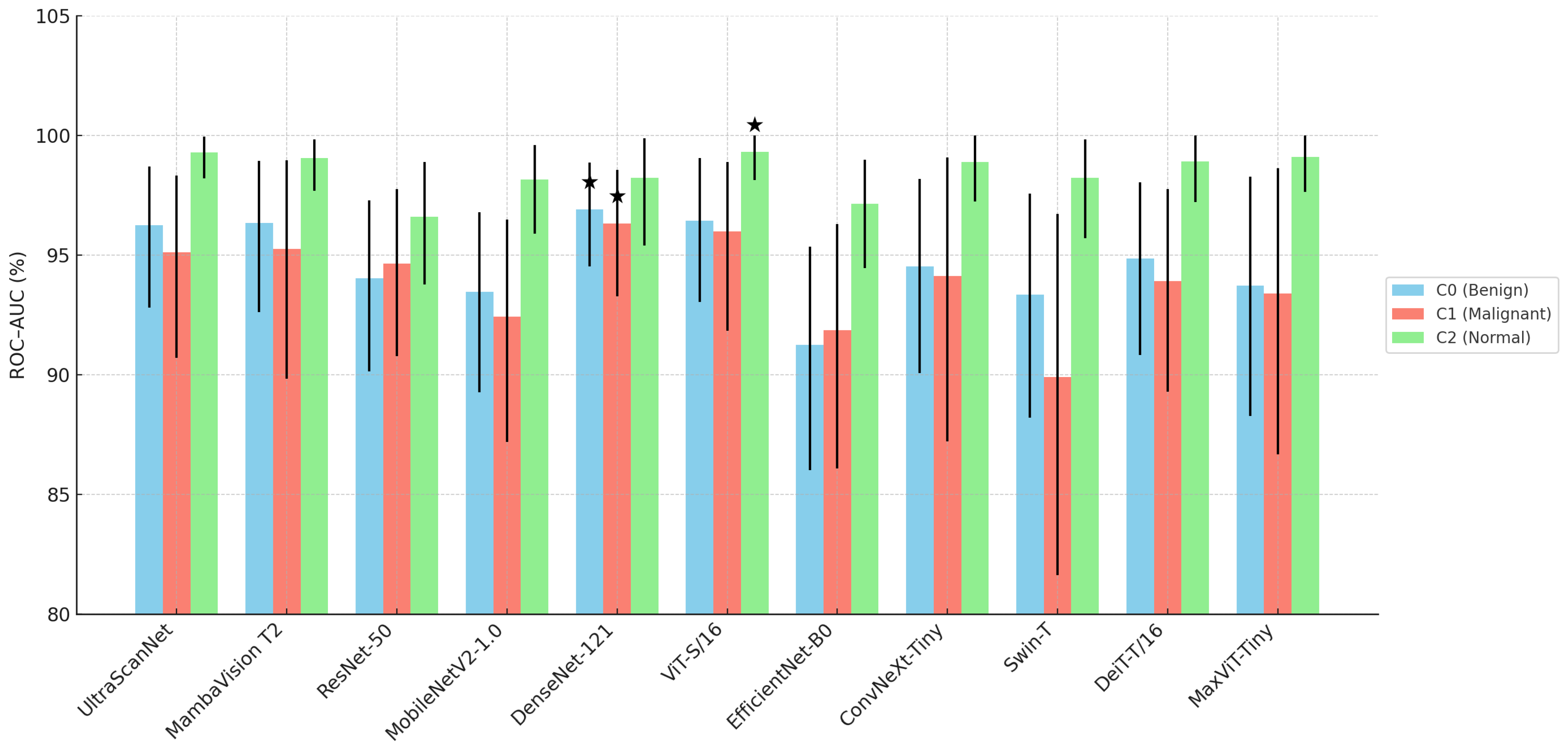
The AUC CIs in

Table 8. Per-class ROC–AUC mean and 95% confidence intervals on BUSI. Classes: C0 = benign, C1 = malignant, C2 = normal. Best value in each column is in bold.

Model	AUC Mean			95% CI Low			95% CI High
	C0	C1	C2	C0	C1	C2	C0	C1	C2
UltraScanNet (ours)	96.24	95.10	99.29	92.81	90.69	98.21	98.70	98.32	99.94
MambaVision T2 (baseline)	96.34	95.25	99.05	92.62	89.83	97.68	98.94	98.95	99.83
ResNet-50	94.02	94.63	96.60	90.14	90.76	93.76	97.27	97.76	98.89
MobileNetV2-1.0	93.47	92.43	98.16	89.26	87.18	95.90	96.79	96.48	99.59
DenseNet-121	96.91	96.32	98.22	94.51	93.28	95.39	98.86	98.55	99.87
ViT-S/16	96.43	95.99	99.30	93.03	91.84	98.13	99.06	98.89	100.00
EfficientNet-B0	91.24	91.85	97.15	86.00	86.08	94.45	95.35	96.30	98.99
ConvNeXt-Tiny	94.53	94.12	98.88	90.06	87.20	97.23	98.17	99.07	100.00
Swin-T (patch4, window7)	93.35	89.91	98.23	88.21	81.62	95.71	97.56	96.71	99.82
DeiT-T/16	94.84	93.91	98.91	90.82	89.28	97.21	98.03	97.76	100.00
MaxViT-Tiny	93.71	93.40	99.10	88.26	86.66	97.63	98.27	98.62	100.00

and in Figure 16 reflect the ranking ability—the model’s capacity to separate positive from negative samples regardless of the decision threshold—while accounting for uncertainty.

• Benign (C0): DenseNet-121 holds the top AUC mean (96.91%) and the highest lower bound (94.51%), making it the most consistent separator for benign cases.
• Malignant (C1): DenseNet-121 again leads with a 96.32% mean and 93.28% lower bound, showing excellent and stable discriminative power for malignant lesions.
• Normal (C2): ViT-S/16 achieves the highest mean (99.30%) and the highest lower bound (98.13%), which confirms its ability to distinguish normal tissue from pathologies.

Overall, while different architectures peak in different classes, UltraScanNet demonstrates a competitive balance: perfect recall in normal (C2), a high AUC in the benign and malignant classes, and consistently narrow CIs. This suggests that it can serve as a strong all-rounder, whereas DenseNet-121 excels in benign/malignant discrimination and ViT-S/16 shows strengths in normal tissue separation.

5.8. Confusion Matrices

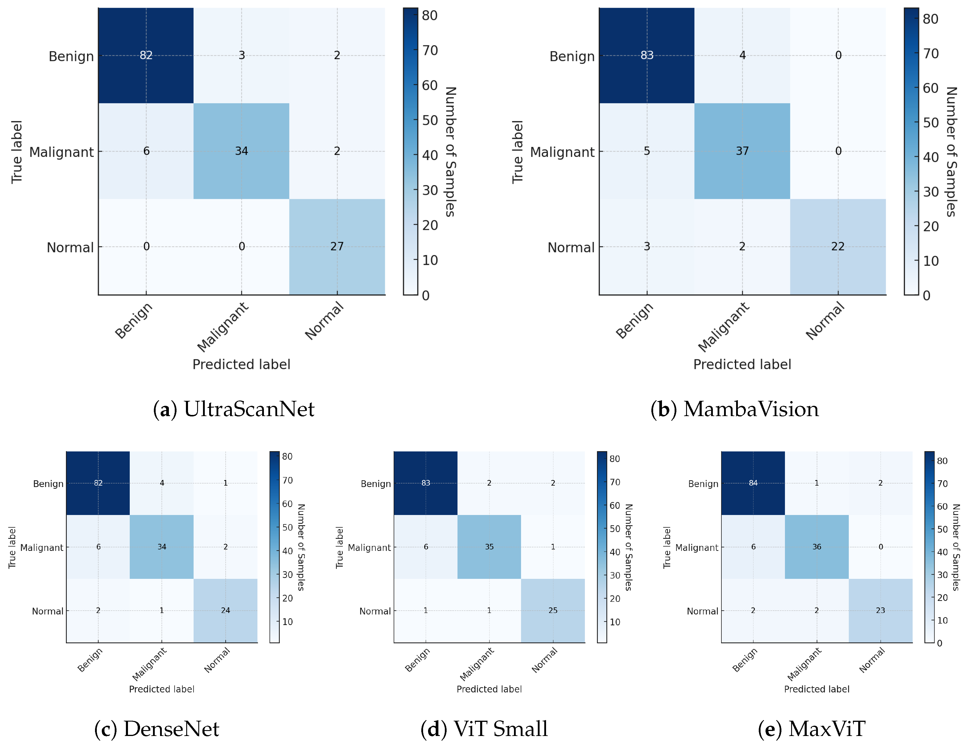
Figure 17 shows that UltraScanNet achieves 100% accuracy for normal (27/27) while maintaining high benign detection (82/87, 94.3%) but shows moderate malignant detection (34/42, 81.0%). On the other hand, MambaVision achieves better malignant sensitivity (37/42, 88.1%) but loses normal recall (22/27, 81.5%), indicating the occasional confusion of normal tissue with lesions. DenseNet mirrors UltraScanNet’s malignant recall (34/42, 81.0%) and slightly weaker normal recall (24/27, 88.9%). ViT Small provides a balanced profile (benign 95.4%, malignant 83.3%, normal 92.6%), distributing the errors more evenly across classes. MaxViT achieves the highest benign detection rate (84/87, 96.6%) and maintains good malignant detection (36/42, 85.7%), but its normal detection (23/27, 85.2%) falls behind that of ViT Small and UltraScanNet.

The most frequent mistake among models occurs when malignant cases are misclassified as benign because of the clinical difficulty in detecting faint malignant lesions in ultrasound images. UltraScanNet focuses on avoiding normal case misdiagnoses, but MambaVision and MaxViT prioritize malignant sensitivity at the cost of normal specificity.

5.9. Cross-Dataset Evaluation on BUS-UCLM

5.9.1. Top-1 Accuracy, Precision, Recall, and F1-Score

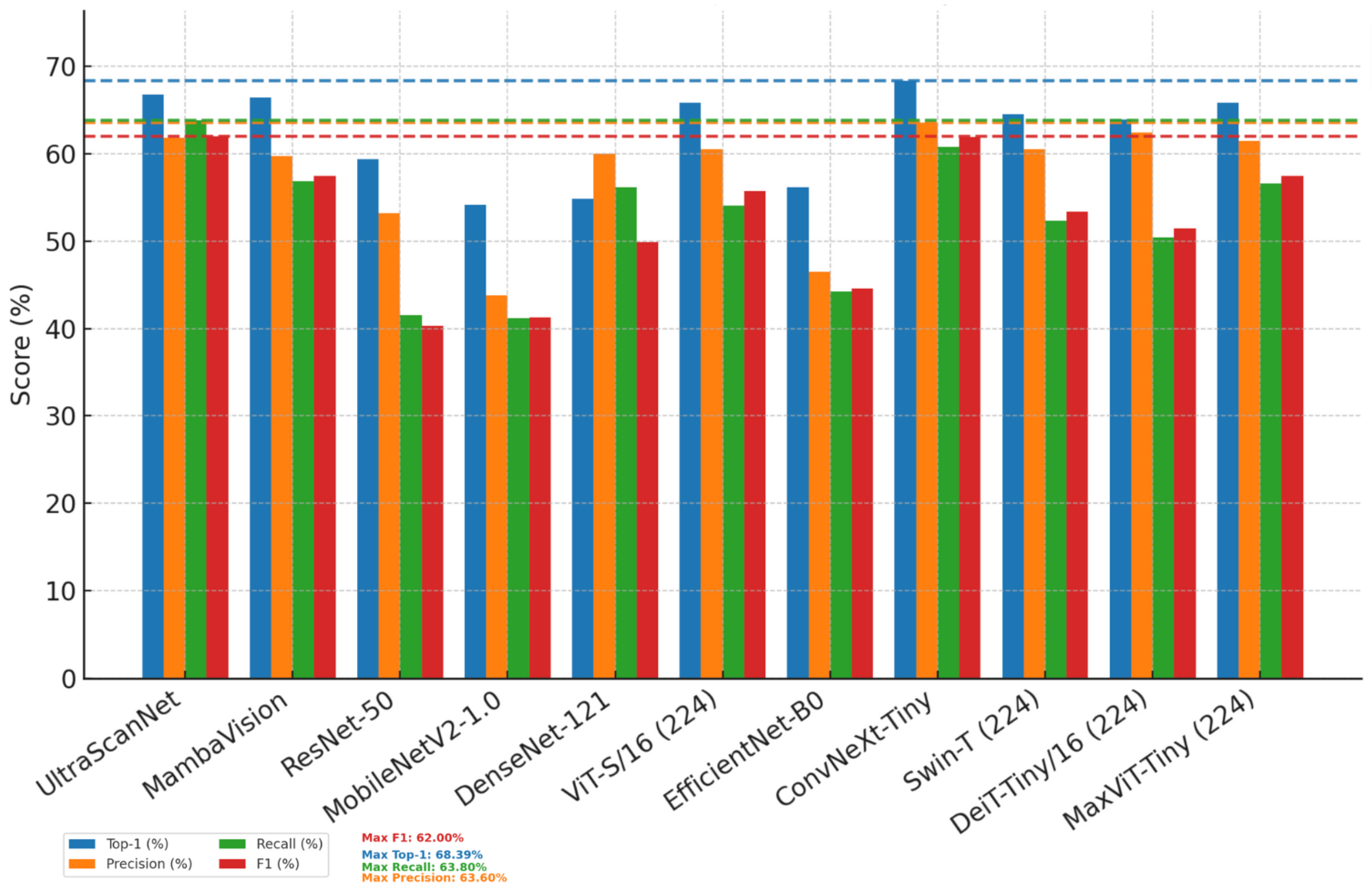
To further assess the generalization capabilities of the proposed architecture, we evaluated UltraScanNet and all comparison models on the BUS-UCLM [48] dataset, a completely different breast ultrasound dataset. We took random samples from the data but maintained the same proportions of the classes as in the BUSI dataset on which the models had been trained. In this experiment, the models were tested directly using their pretrained weights from the BUSI training, with no additional fine-tuning or retraining performed. This setup provides a direct measure of the cross-dataset transferability. The results are provided in

Table 9. BUS-UCLM (balanced) validation results. Best values in bold.

Model	Top-1 (%)	Precision	Recall	F1
UltraScanNet (ours)	66.77	0.618	0.638	0.620
MambaVision	66.45	0.597	0.569	0.575
ResNet-50	59.35	0.532	0.415	0.403
MobileNetV2-1.0	54.19	0.438	0.412	0.413
DenseNet-121	54.84	0.600	0.562	0.499
ViT-S/16 (224)	65.81	0.605	0.541	0.557
EfficientNet-B0	56.13	0.465	0.442	0.446
ConvNeXt-Tiny	68.39	0.636	0.608	0.619
Swin-T (224)	64.52	0.605	0.523	0.534
DeiT-Tiny/16 (224)	63.87	0.624	0.504	0.515
MaxViT-Tiny (224)	65.81	0.615	0.566	0.575

. We also provide a visual representation of the results in Figure 18.

The out-of-the-box evaluation on BUS-UCLM shows that ConvNeXt-Tiny achieves the highest top-1 accuracy (68.39%) and precision (0.636), which indicates strong class discrimination when the predictions are correct. UltraScanNet, on the other hand, leads in recall (0.638) and the macro F1-score (0.620), which reflects more balanced performance across classes and a stronger ability to identify positive cases, especially under domain shift.

This trade-off suggests that, while ConvNeXt-Tiny is slightly better in producing precise predictions, UltraScanNet generates more true positives, which results in the best overall harmonic mean of precision and recall. The fact that our model retains top-tier performance without any additional fine-tuning on this dataset highlights its robustness and adaptability in low-data, cross-domain scenarios.

These results also confirm that UltraScanNet’s design choices, including the learnable 2D positional encodings and depth-aware hybrid blocks, enable robust adaptation to unseen domains and small-sample regimes, making it a suitable candidate for deployment in settings where retraining with large labeled datasets is not feasible.

It should be mentioned that these results were obtained after training only on a small dataset (BUSI), and more extensive training, together with broader data collection and improved data availability, will almost certainly generate better performance.

5.9.2. Per-Class Recall at 95% Confidence Intervals

The confidence intervals show that UltraScanNet’s macro F1-score superiority over MambaVision remains statistically significant even when working with limited data from different domains. The recall performance of UltraScanNet remains strong for benign cases (class 0: 0.759 [0.697, 0.824]) and reaches its highest point for normal cases (class 2: 0.703 [0.574, 0.827]), except for DenseNet-121. MambaVision achieves the highest recall rate for malignant cases (class 1: 0.626 [0.519, 0.724]), yet its normal case recall drops significantly to 0.286 [0.171, 0.406]. The results are provided in

Table 10. The 95% confidence intervals (CI) for the macro F1-score and per-class recall on BUS-UCLM (out-of-the-box). Values are mean [low, high]. Best per column in bold.

Model	F1-Macro	Recall C0	Recall C1	Recall C2
UltraScanNet (ours)	0.620 [0.558, 0.680]	0.759 [0.697, 0.824]	0.459 [0.347, 0.567]	0.703 [0.574, 0.827]
MambaVision	0.575 [0.508, 0.638]	0.800 [0.739, 0.859]	0.626 [0.519, 0.724]	0.286 [0.171, 0.406]
ResNet-50	0.402 [0.344, 0.465]	0.931 [0.891, 0.965]	0.181 [0.092, 0.268]	0.134 [0.046, 0.245]
MobileNetV2-1.0	0.413 [0.355, 0.471]	0.776 [0.713, 0.837]	0.289 [0.190, 0.386]	0.172 [0.075, 0.283]
DenseNet-121	0.498 [0.435, 0.557]	0.605 [0.531, 0.677]	0.253 [0.161, 0.344]	0.831 [0.727, 0.925]
ViT-S/16 (224)	0.558 [0.496, 0.618]	0.863 [0.809, 0.914]	0.458 [0.354, 0.566]	0.307 [0.186, 0.432]
EfficientNet-B0	0.446 [0.388, 0.505]	0.766 [0.703, 0.828]	0.376 [0.268, 0.477]	0.192 [0.094, 0.309]
ConvNeXt-Tiny	0.619 [0.554, 0.677]	0.812 [0.751, 0.866]	0.578 [0.464, 0.690]	0.435 [0.300, 0.575]
Swin-T (224)	0.533 [0.471, 0.596]	0.891 [0.847, 0.937]	0.301 [0.203, 0.402]	0.381 [0.255, 0.513]
DeiT-Tiny/16 (224)	0.516 [0.455, 0.577]	0.909 [0.867, 0.949]	0.267 [0.179, 0.365]	0.345 [0.226, 0.471]
MaxViT-Tiny (224)	0.575 [0.511, 0.638]	0.789 [0.728, 0.845]	0.625 [0.517, 0.733]	0.286 [0.167, 0.408]

.

This demonstrates how UltraScanNet maintains balanced class generalization when dealing with new data, while other architectures show predictions that are more specific to particular categories. The narrow F1-score CIs of UltraScanNet demonstrate its consistent performance during domain shifts, which supports its deployment in standard scenarios.

6. Computational Complexity and Inference Efficiency

We report in

Table 11. Comparison of model complexity and inference time across CNN-, Transformer-, and Mamba-based architectures. FLOPs are computed for a $224\times 224$ input.

Model	Params (M)	FLOPs (G)	Inference Time (ms)
UltraScanNet (ours)	36.48	5.59	5.84
MambaVision	34.44	5.12	5.42
ResNet-50	23.51	4.13	2.16
MobileNetV2-1.0	2.19	0.30	2.26
DenseNet-121	6.87	2.83	5.80
ViT-Small-Patch16-224	21.59	4.25	2.22
EfficientNet-B0	3.97	0.38	2.82
ConvNeXt-Tiny	27.80	4.45	2.83
Swin-Tiny	27.50	4.37	4.45
DeiT-Tiny-Patch16-224	5.49	1.08	2.21
MaxViT-Tiny-RW-224	28.45	4.89	7.60

the number of floating point operations (FLOPs), total trainable parameters, and average inference time per image for all evaluated models on the BUSI dataset. FLOPs are computed for a single forward pass, the parameters are counted in millions, and the inference time is measured in milliseconds on the same hardware configuration.

The analysis of model complexity versus efficiency in Table 11 demonstrates that UltraScanNet strikes an optimal equilibrium between model complexity and deployment feasibility. The model’s parameter count and FLOPs exceed those of its MambaVision backbone, but the resulting computational cost increase remains reasonable, and the system operates within real-time parameters. UltraScanNet outperforms traditional CNNs (ResNet-50, DenseNet-121) and pure Transformer models (ViT-Small, Swin-Tiny) in terms of throughput while maintaining a more complex architecture. The lightweight networks MobileNetV2 and EfficientNet-B0 provide faster inference but compromise their representational capacity, which remains essential for demanding medical imaging applications. The results indicate that UltraScanNet uses its hybrid structure to improve its feature extraction capabilities without compromising its efficiency, which makes it appropriate for clinical settings that require timely operations.

7. Explainability Through Grad-CAM Visualizations

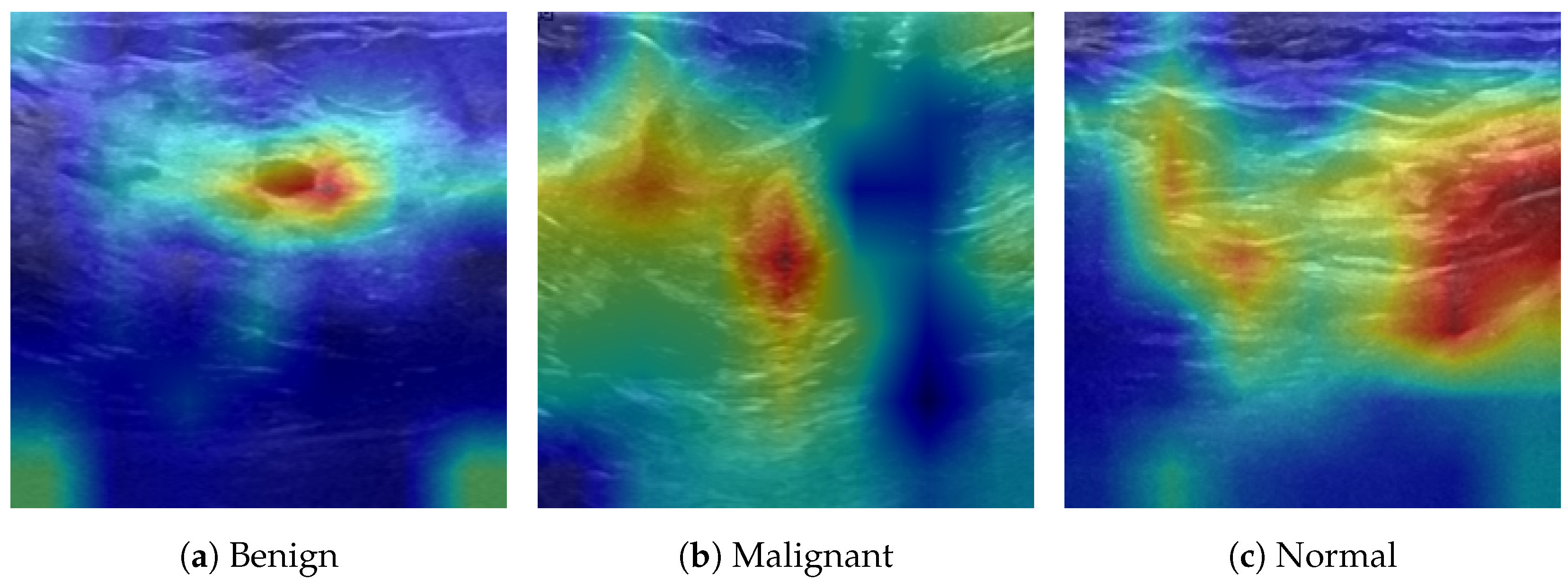
The transparency of the classification results is enhanced through the implementation of gradient-weighted class activation mapping (Grad-CAM) on representative test samples from each class in the BUSI dataset: benign, malignant, and normal tissue. The model uses Grad-CAM to generate class-discriminative localization maps, which show the most important regions in the input image for decision making.

The Grad-CAM outputs for three representative samples are shown in Figure 19.

It can easily be seen how the model directs its activation power toward the lesion boundary in benign cases (left) because it uses boundary and texture information to distinguish between benign and malignant tumors. The next heatmap displays strong activation patterns throughout the lesion core and its irregular extensions, which match the clinically important malignant features of spiculated edges and a heterogeneous echotexture. Lastly, the model distributes its attention across the entire image, without focusing on any specific mass-like region, because there are no suspicious structures present.

This Grad-CAM analysis creates an interpretable connection between network feature representations and raw ultrasound images, which can help clinicians and researchers to trust the model’s predictions.

8. Ablation Studies

To better understand the contributions of each architectural component in UltraScanNet, we conducted a series of targeted ablation studies. These included modifications at different stages of the network—ranging from positional encoding schemes and hybrid token mixers in the early layers to the design of temporal and attention-based modules in deeper stages. Our goal was to isolate the effects of key design choices and justify the final architecture based on empirical evidence.

All experiments were performed under identical training and evaluation conditions on the BUSI dataset to ensure fairness. For reproducibility and to support further research, the codebase—including all custom blocks and training scripts used in this ablation study—will be released in our GitHub repository (https://github.com/Ale0311/UltraScanNet (accessed on 24 July 2025)) in a future update to accompany this work.

8.1. Positional Encoding

This ablation study evaluates the impact of different patch embedding methods and positional encoding approaches on the classification accuracy. The learned 2D positional embedding (PatchEmbedLearnedPos) achieved the highest top-1 accuracy at 91.67%, which demonstrates the critical role of direct spatial encoding for breast ultrasound image classification.

The combination of simple Mamba blocks (linear layer + activation + linear layer) with attention mechanisms (Mamba + Attn) produced similar results (91.03%), which indicates that basic sequence modeling provides some advantages but does not exceed the performance of learned spatial embeddings. Methods that used shallow attention and ConvNeXt-style context and dropout regularization in the embedding stage achieved significantly lower performance because early spatial representations remain fragile. Mobile-style inverted residual blocks together with single-stage positional embeddings failed to perform well because they lacked sufficient representational capacity and spatial detail.

The results (

Table 12. Ablation study: positional encoding.

Variant	Top-1 Accuracy (%)
Patch Embedding + Learned Pos	91.67
Mamba + Attn	91.03
Simple Patch Embedding	90.38
Hybrid ConvNeXt	83.33
Hybrid	82.69
Posemb Patch1Stage	82.69
ConvNeXt + Attn	82.05
Inverted	78.85
Shallow Attn	78.21
Hybrid Dropout	71.79
Learned Pos + Attn	66.03

) demonstrate that models require powerful, spatially sensitive patch embeddings during their initial stages, while cautioning against excessive regularization and early attention layers in low-level model stages.

8.2. Stage 1

We studied how different Stage 1 architectures affected the classification results by replacing the early feature extractor with multiple convolutional, attention-based, and Mamba-style modules. All models had the same patch embedding and hybrid architecture downstream to allow a fair comparison (see

Table 13. Ablation study: Stage 1 configurations. Best value in bold.

Variant	Top-1 Accuracy (%)
ConvBlock
Patch Embed + Learned Pos + ConvBlock + PosEnc	91.67
Patch Embed + Mamba + Attn + ConvBlock + PosEnc	89.10
Patch Embed + ConvBlock + PosEnc	89.10
SE Conv
Patch Embed + SE Conv	88.46
Patch Embed + Learned Pos + SE Conv	88.46
Patch Embed + Mamba + Attn + SE Conv	88.46
ConvNeXt
Patch Embed + Mamba + Attn + ConvBlock + ConvNeXt	85.26
Patch Embed + ConvBlock + ConvNeXt	82.69
Patch Embed + Learned Pos + ConvBlock + ConvNeXt	82.05
ConvBlock + LayerNorm
Patch Embed + Learned Pos + ConvBlock + LN + PosEnc	84.62
Patch Embed + ConvBlock + LN + PosEnc	83.33
Patch Embed + Mamba + Attn + ConvBlock + LN + PosEnc	82.05
Mamba Simple
Patch Embed + Mamba Simple	83.97
Patch Embed + Learned Pos + Mamba Simple	81.41
Patch Embed + Mamba + Attn + Mamba Simple	81.41
ConvMixer
Patch Embed + Mamba + Attn + ConvMixer	82.05
Patch Embed + Learned Pos + ConvMixer	82.05
Patch Embed + ConvMixer	81.41
CoordConv
Patch Embed + CoordConv	80.77
Mamba Hybrid
Patch Embed + Learned Pos + Mamba Hybrid	80.77

).

The best results were achieved with a ConvBlock stage combined with patch embedding and learned positional encoding (91.67% top-1 accuracy), highlighting the importance of early spatial priors and structured feature extraction. The removal of the learned positional embedding or its replacement with shallow Mamba + attention resulted in a moderate performance drop (89.10%).

The variants that used SE attention blocks [53] provided small improvements over standard convolution, but their performance stopped increasing at ∼88.46%. The more advanced token mixing methods, such as Mamba, ConvMixer, and ConvNeXt, performed poorly in Stage 1, with accuracy levels between 81 and 85%. These blocks may not have the spatial inductive bias required for the early visual processing of ultrasound data.

The CoordConv and Mamba hybrid configurations achieved the lowest performance (80.77%), which shows that introducing coordinate channels or combining token mixing with convolutions at this stage may reduce spatial coherence.

Our research indicates that standard convolutions with learned spatial encoding work best for initial processing stages, but advanced global and token mixing methods should be used in deeper layers.

8.3. Stage 2

To assess the impact of the second stage in the feature hierarchy, we conducted an ablation study in which only the second block was varied, while keeping the patch embedding and Stage 1 configuration fixed (Patch Embed + Learned Pos + ConvBlock + PosEnc).

The hybrid module of Stage 2 integrated standard convolutional blocks with MobileViT blocks that used attention-like mechanisms to mix spatial tokens. The design reached its highest accuracy at 91.67% because it effectively combined local and global processing methods for breast ultrasound image structural patterns.

The performance decreased dramatically to 83.97% after replacing the hybrid design with ResMamba blocks, which included low-rank state-space modeling and convolutional residual connections. ResMamba blocks demonstrate poor performance in maintaining crucial spatial details needed for lesion classification, despite their ability to model temporal or global information.

The accuracy decreased further, to 78.21%, when ConvNeXt blocks were used in Stage 2, because depthwise token mixing produced features that became too smooth for medical texture recognition.

The results of this ablation study (

Table 14. Ablation study: Stage 2 block type comparison. Best value in bold.

Stage 2 Block Type	Top-1 Accuracy (%)
Hybrid	91.67
ResMamba	83.97
ConvNeXt	78.21

) show that Stage 2 achieves its best performance by maintaining spatial locality while adding a restricted global context.

8.4. Stage 3 and Mixer Scheduling

In this section, we detail the results of the ablation study of the mixers in the latest stages of the network (

Table 15. Mixer scheduling ablation on BUSI (sorted by top-1). Best value in bold.

Arrangement	Top-1 (%)
Depth-aware hybrid (USM→CAM→MHSA)	91.67
USM → CAM×3 (center) → MHSA	91.03
USM/CAM alternating + MHSA last	90.38
All-USM (scaled late)	90.38
USM → CAM×2 (center) → MHSA	90.38
USM + every 4th block MHSA	89.74
USM → CAM×2 (center) → USM → MHSA×2 (tail)	89.74
MHSA first → USM → CAM (tail)	89.74
All-MHSA (head scaling late)	89.74
All-USM (constant)	89.74
All-MHSA	89.10
MHSA at edges, CAM in the middle	89.10
USM body → MHSA×2 (tail)	88.46
Reversed (MHSA→CAM→USM)	87.82
All-CAM	86.54

). All previous stages are frozen to the best-performing blocks (Patch Embed + Learned Pos and ConvBlock + PosEnc and Hybrid Stage 2).

Within each stage, we assign a mixer type to each block by position.

We experiment with policies consisting of

• USM (UltraScanUnit; state-space + gated conv residuals);
• CAM (ConvAttnMixer; depthwise conv + FFN token mixing);
• and MHSA (multi-head self-attention)

in specific regions of the stage, at specific positions (e.g., last block), or in simple patterns (e.g., alternating, “every 4th”).

Arrangements

• Depth-aware hybrid (USM→CAM→MHSA): USM in the early region (first ∼third of blocks), CAM in the middle region (around the midpoint), MHSA in the late region (last ∼third).
• USM → CAM×3 (center) → MHSA: Three contiguous CAM blocks are placed around the stage midpoint; blocks before them use USM; blocks after them use MHSA.
• USM/CAM alternating + MHSA last: From the start to the penultimate block, USM and CAM alternate; the final block is MHSA.
• All-USM (scaled late): All blocks are USM; later blocks use a larger internal state to modestly increase capacity.
• USM → CAM×2 (center) → MHSA: Two contiguous, midpoint-centered CAM blocks; USM before, MHSA after.
• USM + every 4th block MHSA: Sequence is USM everywhere, except that every fourth block is replaced by MHSA.
• USM → CAM×2 (center) → USM → MHSA×2 (tail): Two centered CAM blocks; early and mid-late regions around them use USM; the last two blocks are MHSA.
• MHSA first → USM → CAM (tail): The very first block is MHSA; up to the last third, the blocks are USM; the final region is CAM.
• All-MHSA (head scaling late): All blocks are attention, with more heads toward the end of the stage.
• All-USM (constant): Every block is USM with the same internal state size.
• All-MHSA: Every block is attention with a fixed head setting.
• MHSA at edges, CAM middle: A thin attention band at the very beginning and end (edges) of the stage; CAM everywhere else.
• USM body → MHSA×2 (tail): All blocks are USM except the last two, which are MHSA.
• Reversed (MHSA→CAM→USM): Attention early, CAM in the middle, USM late.
• All-CAM: Every block uses ConvAttnMixer.

Placing USM early, CAM mid, and MHSA late renders the best result. This happens because USM stabilizes high-resolution feature maps, CAM expands the receptive field efficiently at intermediate resolutions, and MHSA aggregates global semantics when tokens are few. Centering a small CAM window or alternating USM/CAM with a single MHSA tail block recovers most of the global benefit at a lower cost, while attention-heavy schedules (especially with attention early) degrade both the accuracy and efficiency.

9. Conclusions

This paper presents UltraScanNet, a Mamba-inspired hybrid backbone, together with an extensive ablation study of the architecture and an in-depth performance analysis and model comparison. The proposed architecture integrates convolutional inductive priors with lightweight attention mechanisms and temporally aware state-space modeling through UltraScanUnit. The staged hybrid design that combines MobileViT blocks with positional encodings and the depth-aware scheduling of convolutional, SSM, and attention blocks creates an optimal balance between local texture modeling and global context reasoning.

UltraScanNet achieves very competitive performance on the BUSI dataset by matching or surpassing leading CNNs, ViTs, and SSMs in both accuracy and robustness. Ablation studies confirm the significance of each architectural component by demonstrating how learned positional priors, hybrid token mixing, and a modular composition improve low-data grayscale imaging tasks.

Moreover, the value of this work extends beyond the proposed architecture because it includes extensive evaluation transparency. The evaluation provides both global and per-class metrics together with a complete ablation analysis of all layers to explain the design success points and efficiency trade-offs. The detailed analysis of our results transforms them into practical reference materials for future research and deployment, because it offers fair, reproducible comparisons and reveals clinical operating characteristics. These detailed reports aim to provide dependable benchmarks that will guide future research and evaluation efforts in breast ultrasound classification.

For future work, we aim to curate a large, diverse breast ultrasound (BUS) dataset by consolidating multiple publicly available sources and, where possible, incorporating additional clinical contributions. This will allow us to train UltraScanNet on a more representative and comprehensive dataset, addressing the current limitations of small-sample training. We will then continue our research by extending UltraScanNet to perform tasks that go beyond classification, including lesion segmentation and detection. Furthermore, we plan to adapt the model for use in multimodal ultrasound scenarios that include Doppler and elastography imaging, and we will explore self-supervised pretraining and domain adaptation methods to enhance generalization between clinical datasets and imaging devices.

References

1. Liu, L.; Sun, H.; Li, F. A Lie group kernel learning method for medical image classification. Pattern Recognit. 2023, 142, 109735. [Google Scholar] [CrossRef]
2. Yadav, S.S.; Jadhav, S.M. Deep convolutional neural network based medical image classification for disease diagnosis. J. Big Data 2019, 6, 113. [Google Scholar] [CrossRef]
3. Li, Z.; Jiang, J.; Chen, K.; Chen, Q.; Zheng, Q.; Liu, X.; Weng, H.; Wu, S.; Chen, W. Preventing corneal blindness caused by keratitis using artificial intelligence. Nat. Commun. 2021, 12, 3738. [Google Scholar] [CrossRef] [PubMed]
4. Hoang, D.-T.; Shulman, E.D.; Turakulov, R.; Abdullaev, Z.; Singh, O.; Campagnolo, E.M.; Lalchungnunga, H.; Stone, E.A.; Nasrallah, M.P.; Ruppin, E.; et al. Prediction of DNA methylation-based tumor types from histopathology in central nervous system tumors with deep learning. Nat. Med. 2024, 30, 1952–1961. [Google Scholar] [CrossRef]
5. Zhang, X.; Zhao, Z.; Wang, R.; Chen, H.; Zheng, X.; Liu, L.; Lan, L.; Li, P.; Wu, S.; Cao, Q.; et al. A multicenter proof-of-concept study on deep learning-based intraoperative discrimination of primary central nervous system lymphoma. Nat. Commun. 2024, 15, 3768. [Google Scholar] [CrossRef] [PubMed]
6. Huang, S.-C.; Pareek, A.; Jensen, M.; Lungren, M.P.; Yeung, S.; Chaudhari, A.S. Self-supervised learning for medical image classification: A systematic review and implementation guidelines. NPJ Digit. Med. 2023, 6, 74. [Google Scholar] [CrossRef] [PubMed]
7. Li, Z.; Zhang, X.; Müller, H.; Zhang, S. Large-scale retrieval for medical image analytics: A comprehensive review. Med. Image Anal. 2018, 43, 66–84. [Google Scholar] [CrossRef]
8. Yang, Y.; Hu, Y.; Zhang, X.; Wang, S. Two-stage selective ensemble of CNN via deep tree training for medical image classification. IEEE Trans. Cybern. 2021, 52, 9194–9207. [Google Scholar] [CrossRef]
9. Chen, X.; Wang, X.; Zhang, K.; Fung, K.-M.; Thai, T.C.; Moore, K.; Mannel, R.S.; Liu, H.; Zheng, B.; Qiu, Y. Recent advances and clinical applications of deep learning in medical image analysis. Med. Image Anal. 2022, 79, 102444. [Google Scholar] [CrossRef]
10. Fujita, H. AI-based computer-aided diagnosis (AI-CAD): The latest review to read first. Radiol. Phys. Technol. 2020, 13, 6–19. [Google Scholar] [CrossRef]
11. Park, C.-W.; Seo, S.W.; Kang, N.; Ko, B.; Choi, B.W.; Park, C.M.; Chang, D.K.; Kim, H.; Kim, H.; Lee, H.; et al. Artificial intelligence in health care: Current applications and issues. J. Korean Med. Sci. 2020, 35, e379. [Google Scholar] [CrossRef] [PubMed]
12. Wang, W.; Liang, D.; Chen, Q.; Iwamoto, Y.; Han, X.-H.; Zhang, Q.; Hu, H.; Lin, L.; Chen, Y.-W. Medical image classification using deep learning. In Deep Learning in Healthcare: Paradigms and Applications; Springer: Berlin/Heidelberg, Germany, 2020; pp. 33–51. [Google Scholar]
13. Ashraf, R.; Habib, M.A.; Akram, M.; Latif, M.A.; Malik, M.S.A.; Awais, M.; Dar, S.H.; Mahmood, T.; Yasir, M.; Abbas, Z. Deep convolution neural network for big data medical image classification. IEEE Access 2020, 8, 105659–105670. [Google Scholar] [CrossRef]
14. Manzari, O.N.; Ahmadabadi, H.; Kashiani, H.; Shokouhi, S.B.; Ayatollahi, A. MedViT: A robust vision transformer for generalized medical image classification. Comput. Biol. Med. 2023, 157, 106791. [Google Scholar] [CrossRef] [PubMed]
15. Cheng, J.; Tian, S.; Yu, L.; Gao, C.; Kang, X.; Ma, X.; Wu, W.; Liu, S.; Lu, H. ResGANet: Residual group attention network for medical image classification and segmentation. Med. Image Anal. 2022, 76, 102313. [Google Scholar] [CrossRef]
16. World Health Organization. Breast Cancer Fact Sheet. World Health Organization. Available online: https://www.who.int/news-room/fact-sheets/detail/breast-cancer (accessed on 24 July 2025).
17. Berg, W.A.; Blume, J.D.; Cormack, J.B.; Mendelson, E.B.; Lehrer, D.; Böhm-Vélez, M.; Pisano, E.D.; Jong, R.A.; Evans, W.P.; Morton, M.J.; et al. Combined screening with ultrasound and mammography vs mammography alone in women at elevated risk of breast cancer. JAMA 2008, 299, 2151–2163. Available online: https://pubmed.ncbi.nlm.nih.gov/18477782/ (accessed on 24 July 2025). [CrossRef]
18. Al-Dhabyani, W. Dataset of breast ultrasound images. Data Brief 2019, 28, 104863. Available online: https://www.sciencedirect.com/science/article/pii/S2352340919312181 (accessed on 24 July 2025). [CrossRef]
19. Guo, R.; Lu, G.; Qin, B.; Fei, B. Ultrasound imaging technologies for breast cancer detection and management: A Review. Ultrasound Med. Biol. 2015, 44, 37–70. Available online: https://pubmed.ncbi.nlm.nih.gov/29107353/ (accessed on 24 July 2025). [CrossRef]
20. Krizhevsky, A.; Sutskever, I.; Hinton, G.E. ImageNet classification with deep convolutional neural networks. Adv. Neural Inf. Process. Syst. 2012, 25, 1097–1105. [Google Scholar] [CrossRef]
21. He, K.; Zhang, X.; Ren, S.; Sun, J. Deep residual learning for image recognition. In Proceedings of the IEEE Conference on Computer Vision and Pattern Recognition, Las Vegas, NV, USA, 27–30 June 2016; pp. 770–778. [Google Scholar]
22. Vaswani, A.; Shazeer, N.; Parmar, N.; Uszkoreit, J.; Jones, L.; Gomez, A.N.; Kaiser, Ł.; Polosukhin, I. Attention is all you need. Adv. Neural Inf. Process. Syst. 2017, 30, 5998–6008. [Google Scholar]
23. Dosovitskiy, A.; Beyer, L.; Kolesnikov, A.; Weissenborn, D.; Zhai, X.; Unterthiner, T.; Dehghani, M.; Minderer, M.; Heigold, G.; Gelly, S.; et al. An image is worth 16 × 16 words: Transformers for image recognition at scale. arXiv 2020. Available online: https://arxiv.org/abs/2010.11929 (accessed on 24 July 2025).
24. Gu, A.; Dao, T. Mamba: Linear-time sequence modeling with selective state spaces. arXiv 2024. Available online: https://arxiv.org/abs/2312.00752 (accessed on 24 July 2025).
25. Hatamizadeh, A.; Kautz, J. MambaVision: A Hybrid Mamba-Transformer Vision Backbone. In Proceedings of the Computer Vision and Pattern Recognition Conference, Nashville, TN, USA, 11–15 June 2025; pp. 25261–25270. [Google Scholar]
26. Rakhlin, A.; Shvets, A.; Iglovikov, V.; Kalinin, A.A. Deep CNNs for breast cancer histology image analysis. In Image Analysis and Recognition; Springer: Berlin/Heidelberg, Germany, 1970; Available online: https://link.springer.com/chapter/10.1007/978-3-319-93000-8_83 (accessed on 24 July 2025).
27. Huang, G.; Liu, Z.; Van Der Maaten, L.; Weinberger, K.Q. Densely connected convolutional networks. In Proceedings of the IEEE Conference on Computer Vision and Pattern Recognition (CVPR), Honolulu, HI, USA, 21–26 July 2017; pp. 2261–2269. [Google Scholar] [CrossRef]
28. Liu, Z.; Mao, H.; Wu, C.-Y.; Feichtenhofer, C.; Darrell, T.; Xie, S. A convnet for the 2020s. In Proceedings of the IEEE/CVF Conference on Computer Vision and Pattern Recognition, New Orleans, LA, USA, 19–24 July 2022; pp. 11976–11986. [Google Scholar]
29. Radosavovic, I.; Kosaraju, R.P.; Girshick, R.; He, K.; Dollár, P. Designing network design spaces. In Proceedings of the IEEE/CVF Conference on Computer Vision and Pattern Recognition, Seattle, WA, USA, 13–19 June 2020; pp. 10428–10436. [Google Scholar]
30. Tan, M.; Le, Q. EfficientNetV2: Smaller models and faster training. Int. Conf. Mach. Learn. 2021, 38, 10096–10106. [Google Scholar]
31. Touvron, H.; Cord, M.; Douze, M.; Massa, F.; Sablayrolles, A.; Jégou, H. Training data-efficient image transformers & distillation through attention. Int. Conf. Mach. Learn. 2021, 38, 10347–10357. [Google Scholar]
32. Liu, Z.; Lin, Y.; Cao, Y.; Hu, H.; Wei, Y.; Zhang, Z.; Lin, S.; Guo, B. Swin transformer: Hierarchical vision transformer using shifted windows. In Proceedings of the IEEE/CVF International Conference on Computer Vision, Montreal, QC, Canada, 10–17 October 2021; pp. 10012–10022. [Google Scholar]
33. Chu, X.; Tian, Z.; Wang, Y.; Zhang, B.; Ren, H.; Wei, X.; Xia, H.; Shen, C. Twins: Revisiting the design of spatial attention in vision transformers. Adv. Neural Inf. Process. Syst. 2021, 34, 9355–9366. [Google Scholar]
34. Wang, W.; Xie, E.; Li, X.; Fan, D.-P.; Song, K.; Liang, D.; Lu, T.; Luo, P.; Shao, L. Pyramid vision transformer: A versatile backbone for dense prediction without convolutions. In Proceedings of the IEEE/CVF International Conference on Computer Vision, Montreal, QC, Canada, 10–17 October 2021; pp. 568–578. [Google Scholar]
35. Li, J.; Xia, X.; Li, W.; Li, H.; Wang, X.; Xiao, X.; Wang, R.; Zheng, M.; Pan, X. Next-ViT: Next generation vision transformer for efficient deployment in realistic industrial scenarios. arXiv 2022, arXiv:2207.05501. [Google Scholar]
36. Xu, W.; Xu, Y.; Chang, T.; Tu, Z. Coscale conv-attentional image transformers. In Proceedings of the IEEE/CVF International Conference on Computer Vision, Montreal, QC, Canada, 10–17 October 2021; pp. 9981–9990. [Google Scholar]
37. Chen, C.-F.R.; Fan, Q.; Panda, R. CrossViT: Cross-attention multi-scale vision transformer for image classification. In Proceedings of the IEEE/CVF International Conference on Computer Vision, Montreal, QC, Canada, 10–17 October 2021; pp. 357–366. [Google Scholar]
38. Mehta, S.; Rastegari, M. MobileViT: Light-weight, mobile-friendly vision transformer. arXiv 2022. Available online: https://arxiv.org/abs/2110.02178 (accessed on 24 July 2025).
39. Hatamizadeh, A.; Heinrich, G.; Yin, H.; Tao, A.; Alvarez, J.M.; Kautz, J.; Molchanov, P. FasterViT: Fast Vision Transformers with Hierarchical Attention. In Proceedings of the International Conference on Learning Representations (ICLR), Vienna, Austria, 7–11 May 2024; Available online: https://arxiv.org/abs/2306.06189 (accessed on 24 July 2025).
40. Li, Y.; Yuan, G.; Wen, Y.; Hu, J.; Evangelidis, G.; Tulyakov, S.; Wang, Y.; Ren, J. EfficientFormer: Vision transformers at MobileNet speed. Adv. Neural Inf. Process. Syst. 2022, 35, 12934–12949. [Google Scholar]
41. Zhu, L.; Liao, B.; Zhang, Q.; Wang, X.; Liu, W.; Wang, X. Vision mamba: Efficient visual representation learning with bidirectional state space model. In Proceedings of the 41st International Conference on Machine Learning, Vienna, Austria, 21–27 July 2024; pp. 62429–62442. [Google Scholar]
42. Liu, Y.; Tian, Y.; Zhao, Y.; Yu, H.; Xie, L.; Wang, Y.; Ye, Q.; Liu, Y. VMamba: Visual State Space Model. NeurIPS Poster. 2025. Available online: https://nips.cc/virtual/2024/poster/94617 (accessed on 24 July 2025).
43. Pei, X.; Huang, T.; Xu, C. EfficientVMamba: Atrous Selective Scan for Light Weight Visual Mamba. In Proceedings of the AAAI Conference on Artificial Intelligence, Vancouver, BC, USA, 20–28 February 2024. [Google Scholar]
44. Patro, B.N.; Agneeswaran, V.S. SIMBA: Simplified Mamba-based architecture for vision and multivariate time series. arXiv 2024, arXiv:2403.15360. [Google Scholar]
45. Ioffe, S.; Szegedy, C. Batch normalization: Accelerating deep network training by reducing internal covariate shift. Int. Conf. Mach. Learn. 2015, 37, 448–456. [Google Scholar]
46. Agarap, A.F. Deep learning using rectified linear units (ReLU). arXiv 2018, arXiv:1803.08375. [Google Scholar]
47. Hendrycks, D.; Gimpel, K. Gaussian error linear units (GELUs). arXiv 2016, arXiv:1606.08415. [Google Scholar]
48. Vallez, N.; Bueno, G.; Deniz, O.; Rienda, M.A.; Pastor, C. BUS-UCLM: Breast ultrasound lesion segmentation dataset. Mendeley Data 2025, V3. [Google Scholar] [CrossRef] [PubMed]
49. Deng, J.; Dong, W.; Socher, R.; Li, L.-J.; Li, K.; Fei-Fei, L. ImageNet: A large-scale hierarchical image database. In Proceedings of the IEEE Conference on Computer Vision and Pattern Recognition, Miami, FL, USA, 20–25 June 2009; pp. 248–255. [Google Scholar] [CrossRef]
50. Tu, Z.; Talebi, H.; Zhang, H.; Yang, F.; Milanfar, P.; Bovik, A.; Li, Y. MaxViT: Multi-Axis Vision Transformer; Springer Nature: Cham, Switzerland, 2022; Available online: https://link.springer.com (accessed on 24 July 2025).
51. Tan, M.; Le, Q.V. EfficientNet: Rethinking Model Scaling for Convolutional Neural Networks. In Proceedings of the 36th International Conference on Machine Learning (ICML 2019), Long Beach, CA, USA, 9–15 June 2019; pp. 6105–6114. Available online: http://proceedings.mlr.press/v97/tan19a.html (accessed on 24 July 2025).
52. Sandler, M.; Howard, A.; Zhu, M.; Zhmoginov, A.; Chen, L.-C. MobileNetV2: Inverted Residuals and Linear Bottlenecks. In Proceedings of the IEEE/CVF Conference on Computer Vision and Pattern Recognition (CVPR), Salt Lake City, UT, USA, 18–22 June 2018; pp. 4510–4520. [Google Scholar] [CrossRef]
53. Hu, J.; Shen, L.; Sun, G. Squeeze-and-Excitation Networks. In Proceedings of the IEEE/CVF Conference on Computer Vision and Pattern Recognition (CVPR), Salt Lake City, UT, USA, 18–22 June 2018; pp. 7132–7141. [Google Scholar] [CrossRef]
Figure 1. The patch embedding layer incorporates learnable 2D positional encoding. The strided convolutions decrease the spatial dimensions, but learnable positional features are incorporated to include spatial priors in the encoding process.
Electronics 14 03633 g001
Figure 2. The Stage 1 architecture implements positional-aware convolutional encoding with learnable 2D embeddings. This stage improves the initial spatial representations before the hybrid modeling process begins.
Electronics 14 03633 g002
Figure 3. The Stage 2 architecture: hybrid local–global encoding via convolutional residual blocks and a MobileViT-based token mixer with spatial gating.
Electronics 14 03633 g003
Figure 4. UltraScanUnit: This block unites state-space operations with convolutional processing and low-rank residual enhancements for adaptive inputs.
Electronics 14 03633 g004
Figure 5. Overview of the proposed UltraScanNet architecture. The model processes an input ultrasound image through a patch embedding layer, followed by four main stages: positional convolutional encoding (Stage 1), hybrid local–global representation (Stage 2), and two progressive context modeling stages (Stage 3) combining UltraScanUnits, ConvAttnMixers, and attention blocks. The final prediction is produced via global pooling and a linear classification head.
Electronics 14 03633 g005
Figure 6. Grouped performance metrics on BUSI. Bars represent top-1 accuracy, precision, recall, and F1-score for each model. Horizontal dashed lines mark the maximum value of each metric across models.
Electronics 14 03633 g006
Figure 7. Comparison of mean accuracy (with standard deviation) between UltraScanNet and MambaVision on BUSI. UltraScanNet achieves slightly higher average accuracy, while both models remain within overlapping variability ranges.
Electronics 14 03633 g007
Figure 8. Per-class F1-scores on BUSI. UltraScanNet attains the highest F1-score for normal (C2), showing a balanced trade-off between precision and recall. Competing models show more class-specific strengths but less consistent balance. The stars indicate the maximum values of per-class metrics.
Electronics 14 03633 g008
Figure 9. Radar comparison of per-class metrics (C0: benign, C1: malignant, C2: normal) for multiple models. Each panel highlights differences in precision, recall, and F1-score.
Electronics 14 03633 g009
Figure 10. Class-wise ROC curves on BUSI. Colors denote C0 (benign), C1 (malignant), and C2 (normal); the dashed diagonal marks random-chance performance. Panels (a,b) show UltraScanNet and MambaVision, while (ce) compare DeiT-T/16, ViT-S/16, and MaxViT-Tiny.
Electronics 14 03633 g010
Figure 11. Precision–recall (PR) curves on BUSI. Each color denotes a class: C0 (benign), C1 (malignant), and C2 (normal). The top row shows UltraScanNet and its baseline, while the bottom row compares DeiT-T/16, ViT-S/16, and MaxViT-Tiny.
Electronics 14 03633 g011
Figure 12. Precision–recall trade-off per class for UltraScanNet. The curves are smoother across all classes, and C1 (malignant) maintains recall at higher thresholds, indicating the more robust detection of malignant cases.
Electronics 14 03633 g012
Figure 13. Precision–recall trade-off per class for the MambaVision baseline model. Precision and recall are relatively stable for C0 (benign) and C2 (normal), but C1 (malignant) shows a sharper recall decline as the threshold increases.
Electronics 14 03633 g013
Figure 14. F1-macro mean with 95% confidence intervals across models on BUSI. UltraScanNet ranks highest, followed closely by ViT-S/16 and MaxViT-Tiny, while lighter convolutional models such as MobileNetV2 and EfficientNet-B0 achieve lower scores.
Electronics 14 03633 g014
Figure 15. Per-class recall with 95% confidence intervals on BUSI. Each color corresponds to a class: C0 (benign), C1 (malignant), C2 (normal). UltraScanNet achieves strong recall across all classes and a more balanced profile, while other competing models show sharper variations. The stars indicate the maximum values of per-class metrics.
Electronics 14 03633 g015
Figure 16. Per-class ROC–AUC with 95% confidence intervals on BUSI. Each color corresponds to a class: C0 (benign), C1 (malignant), C2 (normal). Most models achieve high AUC values above 90%, with UltraScanNet and the Transformer-based methods showing strong separability across all classes. The stars indicate the maximum values of per-class metrics.
Electronics 14 03633 g016
Figure 17. Confusion matrices on the BUSI validation split. Rows represent true labels and columns represent predicted labels for the three classes: benign, malignant, and normal.
Electronics 14 03633 g017
Figure 18. Model performance comparison on the BUS-UCLM dataset. Bars show top-1 accuracy, precision, recall, and F1-score for each model. UltraScanNet achieves the best recall, F1-score, and overall balance, while other models show stronger performance in individual metrics.
Electronics 14 03633 g018
Figure 19. Grad-CAM visualizations for representative BUSI samples. Red/yellow denote the regions that are the most influential for the model’s decisions.
Electronics 14 03633 g019