A Short-Term User-Side Load Forecasting Method Based on the MCPO-VMD-FDFE Decomposition-Enhanced Framework

Abstract

With the transition of the energy structure and the continuous development of smart grids, short-term user-side load forecasting plays a key role in fine power dispatch and efficient system operation. However, existing parameter optimization methods lack multi-dimensional and physically interpretable fitness evaluation. They also fail to fully exploit frequency-domain features of decomposed modal components. These limitations reduce model accuracy and robustness in complex scenarios. To address this issue, this paper proposes a short-term user-side load forecasting method based on the MCPO-VMD-FDFE decomposition-enhanced framework. Firstly, a multi-dimensional fitness function is designed using indicators such as modal energy entropy and energy concentration. The Crested Porcupine Optimizer with Multidimensional Fitness Function (MCPO) algorithm is applied in VMD (Variational Mode Decomposition) to optimize the number of decomposition modes (K) and the penalty factor (α), thereby improving decomposition quality. Secondly, each IMF component obtained from VMD is analyzed by FFT. Key frequency components are selectively enhanced based on adaptive thresholds and weight coefficients to improve feature expression. Finally, a multi-scale convolution module is added to the PatchTST model to enhance its ability to capture local and multi-scale temporal features. The enhanced IMF components are fed into the improved model for prediction, and the final output is obtained by aggregating the results of all components. Experimental results show that the proposed method achieves the best performance on user-side load datasets for weekdays, Saturdays, and Sundays. The RMSE is reduced by 45.65% overall, confirming the effectiveness of the proposed approach in short-term user-side load forecasting tasks.

1. Introduction

Short-term user-side load forecasting serves as an essential tool for power system dispatching, operational optimization, and demand-side management [1,2,3]. It provides accurate load demand information to power utilities, enabling optimized generation planning, reduced operational costs, and improved system reliability and stability. However, with the large-scale integration of distributed energy resources, the volatility and nonlinearity of load sequences have increased significantly, making accurate forecasting more challenging [4,5,6]. Therefore, developing efficient and accurate short-term user-side load forecasting methods holds significant theoretical and practical value [7,8,9].

Traditional load forecasting methods mainly include time series analysis, regression analysis, and exponential smoothing. However, these methods often yield low prediction accuracy and fail to meet the growing demands of modern power grids. In contrast, machine learning and deep learning methods offer better capabilities in handling complex nonlinear relationships and large-scale data. Reference [10] proposed a day-ahead net load forecasting method based on iTransformer to address challenges posed by high penetration of renewable energy. This approach considers components such as photovoltaic generation, wind power, and active loads, demonstrating high accuracy and stable performance. Reference [11] introduced a short-term load forecasting method under electricity market conditions, incorporating real-time electricity prices. This method effectively captures the correlation between price and load, thereby improving prediction accuracy. To address the increasing diversity and randomness of loads in new power systems, Reference [12] proposed a multi-step short-term load forecasting method based on user group segmentation. The results show that the method significantly improves forecasting accuracy and stability across the entire user group. Reference [13] developed a short-term load forecasting model based on Bi-directional LSTM for multiple buildings. The model enhances the representation of unstable peaks and inter-building correlations. Experimental results show substantial improvements in RMSE and MAE compared to traditional LSTM. Reference [14] proposed a short-term forecasting model based on residual-stacked frequency attention to improve load forecasting accuracy in low-voltage distribution networks. This model highlights the main trend features of load signals and outperforms existing deep learning models on multiple datasets in terms of prediction accuracy. Reference [15] proposed TransformGraph, a Transformer-based model that integrates graph convolutional networks (GCNs) to improve electricity net load forecasting. By encoding correlations through GCN and capturing temporal dependencies with self-attention, the model demonstrated superior accuracy and stability compared with five baseline approaches on OPSD datasets from three countries. Reference [16] explored the application of one-dimensional CNNs based on modified Video Pixel Networks (VPNs) for short-term load forecasting, addressing the limited use of CNNs compared with LSTM and GRU in time series problems. Experiments on real-world datasets for 1-h-ahead and 24-h-ahead tasks showed that the proposed CNN model achieved the best overall performance, with 2.21% MAPE for 24-h predictions.

However, due to the large-scale integration of distributed energy resources, the nonlinearity and nonstationarity of load variations have intensified. Relying on a single forecasting model has clear limitations. Constructing a hybrid framework that combines decomposition and prediction can effectively improve forecasting accuracy and robustness while also reducing the risk of overfitting. Reference [17] developed an ensemble forecasting model based on optimized variational mode decomposition (VMD), an improved sand cat swarm algorithm, and a bi-directional long short-term memory (Bi-LSTM) network. The model introduces the beluga whale algorithm to optimize the number of decomposition layers and the penalty factor, leading to enhanced forecasting stability. Reference [18] proposed a hybrid forecasting model combining VMD and support vector regression (SVR), integrating a chaotic mapping mechanism and an improved grey wolf optimizer (CGWO) to optimize SVR parameters. This approach alleviates premature convergence and enhances the exploration ability of the solution space, thus improving forecasting accuracy. To enhance the accuracy of residential load forecasting, Reference [19] introduced a combined deep learning model that considers multi-scale electricity usage behavior of individual households. The model integrates backpropagation neural networks, extreme gradient boosting, and LSTM, achieving stable and accurate load forecasts. Reference [20] presented a combined short-term load forecasting model based on empirical mode decomposition (EMD), extended Kalman filtering, and kernel-based extreme learning machines. Case studies on user-side microgrids demonstrate the model’s accuracy, update stability, and computational efficiency. Reference [21] proposed a hybrid forecasting method for air-conditioning cooling loads, combining VMD and an improved least squares support vector machine (LSSVM). Whale optimization was employed for parameter tuning, enabling effective decomposition of load sequences. Results show the method provides high prediction accuracy and robustness. Reference [22] proposed a short-term load forecasting method combining ICEEMDAN-RLMD dual decomposition with a CrossInformer architecture. The approach employs intelligent optimization for feature selection, integrates multi-granularity patch inputs and multiple attention mechanisms to enhance sequence modeling, and applies SHAP to improve interpretability. Experimental results demonstrate superior accuracy and stability compared with traditional models. Reference [23] developed an ultra-short-term load forecasting model integrating IVMD–SGMD decomposition with BiLSTM enhanced by temporal pattern attention, optimized by INGO. A TCN-based error correction module further improved accuracy, and experiments on quarterly datasets confirmed the model’s high precision and robustness. Despite these advances, two critical challenges remain. First, most optimization algorithms guiding modal decomposition lack multi-dimensional and physically interpretable fitness evaluation, which hinders the effective identification of modal components. Second, the processing of decomposed signals typically remains at the raw input level, without further exploration of their frequency-domain features.

To address the above issues, this paper proposes a short-term user-side load forecasting method based on the MCPO-VMD-FDFE decomposition-enhanced framework. The main contributions of this study are as follows:

• A modal decomposition parameter optimization method driven by a multi-dimensional, physically interpretable fitness function is proposed. A fitness function is designed by integrating modal energy entropy, orthogonality, and dominant frequency concentration. Combined with the Crested Porcupine Optimizer with Multidimensional Fitness Function (MCPO), the method jointly optimizes the VMD parameters, significantly improving decomposition quality and physical interpretability.
• A frequency-domain feature enhancement mechanism based on adaptive thresholding and weighted strategies is introduced. Key frequency components are selected using FFT spectral analysis and adaptive thresholding, followed by selective enhancement based on peak significance weighting. This approach effectively strengthens the frequency-domain expressiveness of the modal components.
• An MSCPatchTST model is constructed by integrating a multi-scale convolution module with channel independence. While maintaining the channel independence advantage of PatchTST, the model introduces parallel 1D convolutions at different scales to extract multi-granularity local features. An adaptive fusion mechanism further enhances the model’s ability to capture both local and multi-scale dynamic features of load sequences.

2. Methodology

The overall framework of the proposed method is illustrated in Figure 1. First, a multi-dimensional fitness function is constructed, and the MCPO algorithm is applied to jointly optimize the number of decomposition modes K and the penalty factor α in VMD. Second, fast Fourier transform (FFT) is used to perform spectral analysis on the VMD components. Key frequency components are selectively amplified based on adaptive thresholding and a weighted enhancement strategy, thereby improving their frequency-domain representation. Finally, the enhanced modal components are fed into a modified PatchTST model with a multi-scale convolution module. This allows the model to capture both local details and dynamic features across different time scales. The final prediction result is obtained by aggregating the outputs of all modal components.

2.1. MCPO-VMD-FDFE Decomposition-Enhanced Framework

To extract the multi-frequency features embedded in user-side load data and enhance the frequency-domain representation of intrinsic mode functions (IMFs), a comprehensive evaluation function is constructed by integrating modal energy entropy and energy concentration. This replaces the traditional single-objective fitness function. The Crowned Pigs Optimizer (CPO) is then used to optimize the number of decomposition modes K and the penalty factor α in VMD. Meanwhile, FFT is applied to perform spectral analysis on the IMF components. Key frequency components are selectively enhanced based on adaptive thresholds and weighting coefficients, thereby improving the feature expressiveness of the modal components.

2.1.1. VMD

Variational Mode Decomposition (VMD) is an adaptive signal decomposition method that can extract modal components at different frequency scales. It is effective in capturing the multi-scale characteristics and fluctuation patterns of load data. Essentially, VMD formulates a constrained variational problem, as expressed by the following equation:

$$\left\{\begin{array}{c}\underset{\{u_k\}\{{\omega }_k\}}{\min }\{{\displaystyle \sum _{k=1}^k}||{\partial }_t[(\delta (t)+{\displaystyle \frac{\mathrm{j}}{\pi t}})u_k(t)]{\mathrm{e}}^{-\mathrm{j}{\omega }_{k}t}|{|}_2^2\}\\ \mathrm{s}.\mathrm{t}.{\displaystyle \sum _{k=1}^K}{u}_k=f(t)\end{array}\right.$$

(1)

where k represents the total number of modes to be decomposed; ${\partial }_t$ is the t-th order moment deviation, reflecting the time-domain characteristics of the signal; $\delta (t)$ denotes the Dirac distribution function, which ensures the localization of each mode in the time-frequency domain; $u_k$ refers to the k-th intrinsic mode component obtained through decomposition; ${\omega }_k$ is the center frequency associated with each mode; $||.||$ indicates the number of elements computed under the L2 norm; and $f(t)$ is the original input signal to be decomposed.

By introducing a Lagrange multiplier and a quadratic penalty term, the constrained problem can be transformed into an unconstrained optimization problem.

$$\left\{\begin{array}{c}L(\{u_k\},\{{\omega }_k\},\lambda )=\alpha {\displaystyle \sum _{k=1}^k}||{\partial }_t\left[\left(\delta (t)+{\displaystyle \frac{\mathrm{j}}{\pi t}}\right)\odot u_k\right]{\mathrm{e}}^{-\mathrm{j}{\omega }_{k}t}|{|}_2^2+\\ ||f(t)-{\displaystyle \sum _{k=1}^k}{u}_k|{|}_2^2+\lambda (t),f(t)-{\displaystyle \sum _{k=1}^k}{u}_k(t)\end{array}\right.$$

(2)

where $\lambda$ is the Lagrange multiplier; $\alpha$ is the penalty factor; and $\odot$ denotes the convolution operator.

2.1.2. MCPO

(1) CPO

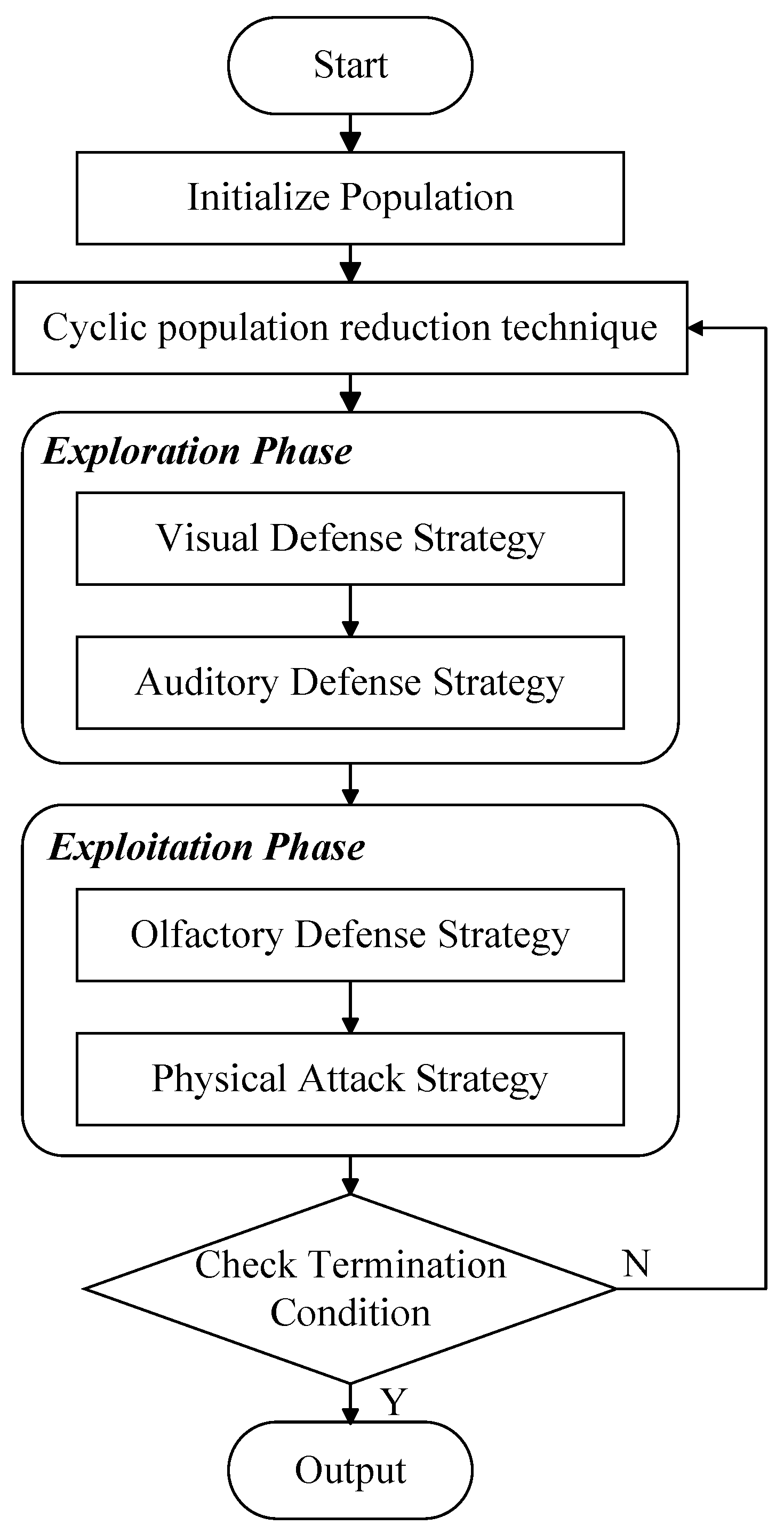
CPO is a novel metaheuristic algorithm. Its flowchart is shown in Figure 2. The algorithm optimizes the objective function by simulating four defensive behaviors of crowned pigs when facing predators. A cyclic population contraction strategy is employed to periodically reduce the number of active individuals during the iteration process. This dynamic reduction in population size accelerates convergence while maintaining population diversity. The initialization process and the formula for cyclic population contraction are defined as follows:

$$\overrightarrow{{\mathrm{X}}_{\mathrm{i}}}=\overrightarrow{\mathrm{L}}+\overrightarrow{\mathrm{r}}\left(\overrightarrow{\mathrm{R}}-\overrightarrow{\mathrm{L}}\right),i=1,2\dots ,n,$$

(3)

$$N=N_{min}+(N^{\prime }-N_{min})\left(1-\left({\displaystyle \frac{t\%\frac{T_{max}}{T}}{\frac{T_{max}}{T}}}\right)\right)$$

(4)

where $n$ denotes the population size; $\overrightarrow{{\mathrm{X}}_{\mathrm{i}}}$ represents the i-th candidate solution in the search space; $\overrightarrow{\mathrm{L}}$ and $\overrightarrow{\mathrm{R}}$ are the upper and lower bounds of the search range, respectively; $\overrightarrow{\mathrm{r}}$ is a random number in the range [0, 1]; T is the predefined cycle period; t denotes the number of function evaluations; $T_{max}$ is the maximum value of the evaluation function; $\%$ represents the remainder or modulo operator, and $N_{min}$ is the minimum number of newly generated individuals in the population.

During the search process, CPO divides the update procedure into two phases: exploration and exploitation. The exploration phase includes two strategies: (i) perturbation updates around the global best solution to increase solution diversity and (ii) convergence adjustment using adaptive scaling factors to regulate search speed. The exploitation phase also includes two strategies: (iii) local refinement through information exchange between individuals; (iv) local intensification using directional and defense factors to accelerate convergence and improve solution accuracy.

The mathematical formulations of the four update strategies are given in Equations (5)–(8). These mechanisms work in a complementary manner, providing a balance between global exploration and local exploitation, and enhancing the algorithm’s performance on complex optimization problems.

$${\overrightarrow{x}}_i^{t+1}={\overrightarrow{x}}_i^t+{\tau }_1\times \left|2\times {\tau }_2\times {\overrightarrow{x}}_{CP}^t-{\overrightarrow{y}}_i^t\right|$$

(5)

where ${\overrightarrow{x}}_{CP}^t$ denotes the current optimal solution of the evaluation function; ${\overrightarrow{y}}_i^t$ represents the position of the predator at iteration time t; ${\tau }_1$ is a random value following a normal distribution; and ${\tau }_2$ is a random number within the range [0, 1]

$${\overrightarrow{x}}_i^{t+1}={\overrightarrow{x}}_{CP}^t+(\alpha (1-{\tau }_4)+{\tau }_4)\times \left(\delta \times {\overrightarrow{x}}_{CP}^t-{\overrightarrow{x}}_i^t\right)-{\tau }_5\times \delta \times {\gamma }_t\times {\overrightarrow{F}}_i^t$$

(6)

where ${\overrightarrow{x}}_{CP}^t$ denotes the obtained optimal solution; ${\tau }_4$ is a random value within the range [1, 4]; $\alpha$ is the convergence rate factor; and ${\overrightarrow{F}}_i^t$ represents the average force acting on the crested porcupine (CP).

$${\overrightarrow{x}}_i^{t+1}=\left(1-{\overrightarrow{U}}_1\right)\times {\overrightarrow{x}}_i^t+{\overrightarrow{U}}_1\times \left(\overrightarrow{y}+{\tau }_3\times \left({\overrightarrow{x}}_{r1}^t-{\overrightarrow{x}}_{r2}^t\right)\right)$$

(7)

where ${\overrightarrow{x}}_{r1}^t$ and ${\overrightarrow{x}}_{r2}^t$ are two random integers in the range [1, N], and ${\tau }_3$ is a random number within the range [0, 1].

$${\overrightarrow{x}}_i^{t+1}=\left(1-{\overrightarrow{R}}_1\right)\times {\overrightarrow{x}}_i^t+{\overrightarrow{R}}_1\times \left({\overrightarrow{x}}_{r1}^t+S_i^t\times \left({\overrightarrow{x}}_{r2}^t-{\overrightarrow{x}}_{r3}^t\right)-{\tau }_3\times \delta \times {\gamma }_t\times S_i^t\right)$$

(8)

where ${\overrightarrow{x}}_i^t$ denotes the position of the i-th individual at iteration t; ${\gamma }_t$ is the defense factor; $r3$ is a random value within the range [1, N]; $\delta$ controls the search direction; ${\tau }_3$ is a random number in the range [0, 1]; and $S_i^t$ represents the odor diffusion factor.

(2) Multi-dimensional Fitness Function

To overcome the limitations of single-objective fitness functions in the variational mode decomposition (VMD) of power load signals, this study proposes a multi-dimensional fitness function by integrating modal energy entropy, orthogonality, and dominant frequency distinguishability. An Alpha-based penalty factor is also introduced. A modified MCPO optimization algorithm based on this multi-dimensional fitness function is developed to enhance the decomposition of multi-scale features in both time and frequency domains. This approach ensures that the resulting modes retain clear physical interpretability and structural rationality while significantly improving the stability and robustness of the decomposition process. The specific formulation of the multi-dimensional fitness function is as follows:

(a) Modal Energy Entropy

Modal energy entropy is used to measure the concentration of energy distribution across the decomposed components. A lower entropy value indicates more concentrated energy, suggesting better decomposition performance. In contrast, a higher entropy value may imply modal redundancy and lower decomposition quality.

$${\overrightarrow{x}}_i^{t+1}=\left(1-{\overrightarrow{R}}_1\right)\times {\overrightarrow{x}}_i^t+{\overrightarrow{R}}_1\times \left({\overrightarrow{x}}_{r1}^t+S_i^t\times \left({\overrightarrow{x}}_{r2}^t-{\overrightarrow{x}}_{r3}^t\right)-{\tau }_3\times \delta \times {\gamma }_t\times S_i^t\right)$$

(9)

$$w_i={\displaystyle \frac{{\displaystyle \sum _{n=1}^N}{u}_{i,n}^2}{{\displaystyle \sum _{n=1}^N}{(u_n)}^2}}$$

(10)

where $E_{entropy}$ denotes the modal energy entropy normalized to [0, 1]; $w_i$ is the energy weight of each mode; $u_i$ represents the decomposed modal component; and $k$ is the total number of modes.

(b) Modal Orthogonality

Orthogonality measures the independence and uncorrelated nature between modal components. Complete orthogonality among modes facilitates accurate signal interpretation and modeling. In contrast, a strong correlation between modes may indicate redundancy or signal leakage.

For any two modes $u_i$ and $u_j$, the orthogonality index is calculated as follows:

$$o(i,j)={\displaystyle \frac{|〈u_i,u_j〉|}{N\cdot \sigma (u_i)\cdot \sigma (u_j)}}$$

(11)

The overall score of modal orthogonality is calculated as the average of all pairwise combinations:

$$O={\displaystyle \frac{1}{(\frac{k}{2})}}\sum _{1\le i<j\le k}o(i,j)$$

(12)

where $o(i,j)$ denotes the orthogonality between modal components; $O$ is the overall orthogonality index; $〈u_i,u_j〉$ represents the dot product between $u_i$ and $u_j$; and $\sigma (·)$ is the standard deviation.

(c) Energy Concentration in the Dominant Frequency Band

The energy concentration in the dominant frequency band is used to measure the frequency-domain separability of the modal components. A dispersed distribution of dominant frequencies indicates that load characteristics have been effectively distinguished, enhancing the physical interpretability of the decomposition. In contrast, overlapping dominant frequencies may lead to modal redundancy and reduced decomposition quality.

For each mode, the dominant frequency is identified as the frequency corresponding to the maximum amplitude after applying the fast Fourier transform (FFT). Let the position of the dominant frequency band be denoted as:

$$f_i=argmax(FFT(u_i))$$

(13)

$$U_p={\displaystyle \frac{ Count{\left\{round(f_i)\right\}}_{i=1}^k}{k}}$$

(14)

where $FFT(·)$ denotes the fast Fourier transform; $Count(·)$ represents the deduplication and counting operation; $round(·)$ refers to the numerical discretization process; and $U_p$ is the proportion of unique dominant frequencies, which means the energy concentration in the dominant frequency band.

(d) Alpha Penalty Factor

To prevent excessively high values of α during the optimization process—which may cause the overall decomposition structure to deviate from expectations—an Alpha penalty factor is introduced to constrain abnormal α values. This ensures a balanced trade-off between energy distribution and structural rationality in the decomposition results.

$${\alpha }_p={\displaystyle \frac{{\lambda }_1}{1+exp(-{\lambda }_2(minmax\left(\alpha \right)-{\lambda }_3))}}$$

(15)

where ${\alpha }_p$ denotes the penalty factor; $minmax\left(·\right)$ represents the normalization operation; and ${\lambda }_i$ is the coefficient of the penalty term.

(e) Fitness Function

The final fitness function comprehensively considers multiple indicators, including modal energy entropy, orthogonality, dominant frequency distinguishability, and the Alpha penalty factor. Its formulation is given as follows:

$$F=\left(\gamma E_{entropy}+\left(1-\gamma \right)O\right)U_p{\alpha }_p$$

(16)

where $\gamma$ is the weighting coefficient.

MCPO is selected within the framework to address the challenges of complexity and non-stationarity in processing user-side load data by integrating a multi-dimensional and physically interpretable fitness function. Unlike traditional optimizers that typically rely on a single objective, the MCPO-based method evaluates decomposition quality using criteria such as modal energy entropy, orthogonality, and dominant frequency concentration. This customized evaluation approach ensures that the parameter optimization for VMD not only pursues mathematical performance but also aligns with the physical characteristics of the load data.

2.1.3. Frequency-Domain Feature Enhancement (FDFE)

To further extract the latent frequency-domain features embedded in intrinsic mode functions (IMFs), a frequency-domain feature enhancement (FDFE) module is designed in this study. First, each IMF component is transformed from the time domain to the frequency domain using fast Fourier transform (FFT), and a peak detection algorithm is applied to identify the dominant and significant secondary frequency components. Second, an adaptive weighting strategy is employed to selectively enhance key frequency bands, while a dynamic energy normalization mechanism is introduced to maintain the stability of the time-domain signal. Finally, the enhanced frequency-domain features are fused with the original IMF components and meteorological features to construct a multimodal augmented dataset, providing higher-quality input features for subsequent forecasting models.

(a) Each intrinsic mode function (IMF) is transformed from the time domain to the frequency domain using fast Fourier transform (FFT), and its amplitude spectrum is calculated as follows:

$$U(k)={\displaystyle \sum _{t=0}^{n-1}}u(t)e^{-j2\pi kt/n},\hspace{1em}k=0,1,\dots ,n-1$$

(17)

$$A(k)=|U(k)|=\sqrt{\mathrm{Re}{\{U(k)\}}^2+\mathrm{Im}{\{U(k)\}}^2}$$

(18)

where $u(t)$ is the intrinsic mode function (IMF); $U(k)$ is the complex spectral value of the k-th frequency component corresponding to the IMF; $A(k)$ is the amplitude of the k-th frequency component; and $\mathrm{Re}\{·\}$ and $\mathrm{Im}\{·\}$ represent the real and imaginary parts, respectively.

(b) Significant Peak Detection

The average amplitude within the half-spectrum segment (from DC to the Nyquist frequency) is calculated as follows:

$${\mu }_f={\displaystyle \frac{1}{⌊n/2⌋}}{\displaystyle \sum _{k=0}^{⌊n/2⌋-1}}A(k)$$

(19)

All peak indices satisfying the condition $A(k)\ge {\mu }_f$ are identified and stored in the set $\mathcal{P}$, and the dominant frequency index along with its corresponding amplitude is determined.

$$\mathcal{P}=\{Peak(k|A(k))=True \& A(k)\ge {\mu }_f\}$$

(20)

$$k_m=\arg \underset{k\in \mathcal{P}}{\max }A(k)$$

(21)

$$A_m=A(k_m)$$

(22)

where $Peak(·)$ is the peak detection function, and $argmax(·)$ is the maximum value selection function.

(c) Frequency-Domain Enhancement

Based on the detected dominant and significant secondary frequency components, an adaptive weighting strategy is employed to selectively enhance key frequency bands $U^{\prime }(k)$:

$$U^{\prime }(k)=\left\{\begin{array}{ll}U(k)\left(\begin{array}{c}1+u_1\end{array}\right),\hfill & k=k_m or k=n-k_m\hfill \\ \hfill & \hfill \\ U(k)\left(\begin{array}{c}1+u_2\end{array}\right),\hfill & k\in \mathcal{P}\setminus \{k_m\} \&A(k)>\tau A_m\hfill \\ \hfill & \hfill \\ U(k),\hfill & else\hfill \end{array}\right.$$

(23)

To ensure the stability of the time-domain signal, dynamic energy normalization is applied to the enhanced signal:

$$\tilde{u}(t)={\displaystyle \frac{1}{n}}{\displaystyle \sum _{k=0}^{n-1}}{U}^{\prime }(k){\mathrm{e}}^{j2\pi kt/n},\hspace{1em}t=0,1,\dots ,n-1$$

(24)

$$u^{\prime }(t)=\tilde{u}(t)\times {\displaystyle \frac{{\sigma }_u}{{\sigma }_{\tilde{u}}}}$$

(25)

The enhanced signal is fused with the original intrinsic mode functions (IMFs) and meteorological features to generate the final frequency-domain augmented dataset:

$$X=[u_k,weather]\to X_{fusion}=[u_k,weather,\tilde{u}(t)]$$

(26)

where $u_1$ is the dominant frequency enhancement coefficient; $u_2$ is the secondary frequency enhancement coefficient; $\tau$ is the significance threshold for secondary frequencies; $\tilde{u}(t)$ is the time-domain signal after enhancement; ${\sigma }_u$ and ${\sigma }_{\tilde{u}}$ represent the standard deviations of the original intrinsic mode function and the enhanced signal, respectively; $X$ and $X_{fusion}$ denote the model input data before and after feature enhancement; and $weather$ refers to the original meteorological features.

The originality of the proposed FDFE module does not lie in the FFT operation itself, but in embedding FFT within a task-oriented enhancement framework. Through adaptive thresholding and weighting strategies, FDFE selectively amplifies informative frequency components while suppressing noise and redundancy. This domain-specific adaptation enables the decomposition results to align more effectively with the non-stationary characteristics of user-side load data, thereby providing clearer and more representative features for downstream forecasting tasks.

2.2. MSCPatchTST (PatchTST with Multi-Scale Convolution)

MSCPatchTST uses patches of the time series as input units. By introducing a patching mechanism, the original time series is divided into multiple non-overlapping patches, which overcomes the limitations of traditional step-by-step processing. In addition, multi-scale convolution is incorporated to enhance the model’s ability to capture local and multi-scale information. The architecture of MSCPatchTST is illustrated in Figure 3.

$$X_{1\mathrm{D}}^l=AETFFBlock \left(X_{1\mathrm{D}}^{l-1}\right)+X_{1\mathrm{D}}^{l-1}$$

(27)

2.2.1. Channel Independence

PatchTST adopts channel-independent input for time series, where each variable is processed separately. Its core architecture is a Transformer encoder, which processes a given sequence of data ${\mathrm{x}}_1,\dots ,{\mathrm{x}}_{\mathrm{L}}$ using a look-back window. The sequence ${\mathrm{x}}_1,\dots ,{\mathrm{x}}_{\mathrm{L}}$ is decomposed into M univariate sequences $x(i)=[x1(i),\dots ,xL(i)]\in {ℝ}^{1\times L}$, where $i=1,\dots ,M$. These sequences are independently fed into the Transformer for processing. After computation, the Transformer outputs the final prediction results as follows:

$${\widehat{x}}^{(\mathrm{i})}={\widehat{x}}_{\mathrm{L}+1}^{(\mathrm{i})},\dots ,{\widehat{x}}_{\mathrm{L}+\mathrm{T}}^{(\mathrm{i})}\in {ℝ}^{1\times \mathrm{T}}$$

(28)

2.2.2. Patching

When processing a univariate time series, it is first divided into multiple patches. Let P be the patch length, and S be the stride, i.e., the non-overlapping interval between two consecutive patches. After patching, a patch sequence $x_p^{(i)}\in {ℝ}^{P\times N}$ is generated, where N denotes the number of resulting patches. The calculation is given by the following formula: $N=\left[{\displaystyle \frac{L-P}{S}}\right]+2$, where L is the length of the input sequence.

2.2.3. Multi-Scale Convolution Module

Although PatchTST is effective at capturing global information, its ability to extract local and multi-scale features remains limited. This limitation is particularly evident in time series data, where local details and global trends may vary across different temporal scales. Relying on a single-scale processing approach may result in the loss of valuable information.

To address the above limitations, an MSCBlock is introduced to extract multi-scale features and perform adaptive feature fusion. In addition, a residual connection is incorporated to ensure that the enhanced features retain the original information. The detailed mechanism of the MSCBlock is as follows:

(a) The input is processed using 1D convolutions with different kernel sizes. Suppose there are $K=[k_1,k_2,\dots ,k_K]$ convolutional kernels. For the i-th convolutional layer, the operation is defined as:

$$y_i=Conv1D_{(k_i)}(x_{reshape})$$

(29)

(b) The multi-scale temporal features are concatenated along the convolutional channel dimension:

$$Y_{concat}=Concat(y_1,y_2,\dots ,y_K)$$

(30)

(c) A 1 × 1 convolution is applied in combination with a residual connection to adaptively fuse the multi-scale features.

$$Y_{fused}=ReLU\left(Conv1D_{(1\times 1)}(Y_{concat})\right)$$

(31)

$$Y_{output}=x_{reshape}+Y_{fused}$$

(32)

where $Conv1D\left(\cdot \right)$ denotes the 1D convolution operation; $y_i$ is the output of the i-th convolutional layer; $Y_{concat}$ represents the concatenated multi-scale tensor; $Concat\left(\cdot \right)$ denotes the concatenation operation; $ReLU\left(\cdot \right)$ is the activation function; $Y_{fused}$ is the fused multi-scale feature; and $Y_{output}$ represents the final output feature tensor.

2.2.4. Transformer Encoder

In PatchTST, each patch is first projected into the Transformer hidden space through a trainable linear projection $W_p\in {ℝ}^{\mathcal{D}\times \mathcal{P}}$ and a learnable positional encoding $W_{\mathrm{pos}}\in {ℝ}^{\mathcal{D}\times N}$, enabling better capture of temporal features within patches. Then, a multi-head attention mechanism is applied to transform the processed data into the query (Q), key (K), and value (V) matrices. Finally, a fully connected layer with a linear head is used to generate the final prediction results:

$${\widehat{x}}^{(i)}=\left[{\widehat{x}}_{L+1}^{(i)},\dots ,{\widehat{x}}_{L+T}^{(i)}\right]\in {ℝ}^{1\times T}$$

(33)

3. Examples Analysis

3.1. User-Side Load Data

The experimental data are derived from a publicly available user-side load dataset from a province in China. The dataset includes separate load records for weekdays, Saturdays, and Sundays. The selected time period spans from 2 January 2024 to 17 March 2025, with a sampling interval of 30 min, resulting in a total of 12,576 data points. To eliminate the influence of dimensional inconsistencies among different variables, all input data for the neural network were normalized to the range [−1, 1]. Inverse normalization was then applied to the predicted values in the test set based on the statistical characteristics of the training set. The dataset was split into training, validation, and test sets in a ratio of 6:2:2.

3.2. Model Parameter Settings

The proposed model is implemented in a Python 3.11 environment using the PyTorch 2.3 framework, and all experiments are conducted on a system equipped with a Core™ i5-13500HX CPU (2.50 GHz) and 8 GB of RAM. Given the lack of established theoretical guidelines for hyperparameter selection, the initial parameter settings are determined empirically. These parameters are further fine-tuned based on model performance during subsequent experiments. The final hyperparameters, determined after multiple trials, are summarized in

Table 1. Parameter Settings.

Parameter Name	Parameter Value
Seq len	144
Number of attention heads	8
Epoch	100
Batch size	24
Patience	10
Dropout	0.05
Optimizer	Adam
Learning rate	0.001
Activation function	GELU
Loss function	MSE

.

3.3. Evaluation Metrics

In this study, the model performance is evaluated using three metrics: mean absolute error (MAE), root mean square error (RMSE), and mean absolute percentage error (MAPE). Lower values of MAE, RMSE, and MAPE indicate smaller deviations between the predicted and actual values, reflecting higher prediction accuracy. The corresponding formulations are given in Equations (34)–(36):

$$MAE={\displaystyle \frac{1}{n}}{{\displaystyle \sum }}_{i=1}^n|y_i-y_i^{\prime }|$$

(34)

$$RMSE=\sqrt{{\displaystyle \frac{1}{n}}{\displaystyle \sum _{i=1}^n}{\left(y_i-y_i^{\prime }\right)}^2}$$

(35)

$$MAPE={\displaystyle \frac{1}{n}}{\displaystyle \sum _{i=1}^n}{\displaystyle \frac{|y_i-y_i^{\prime }|}{y_i}}\cdot 100\%$$

(36)

where n denotes the number of data points, $y_i$ represents the actual values, ${y^{\prime }}_i$ denotes the predicted values, and $\overline{y_i}$ is the mean of the actual values.

3.4. MCPO-VMD Decomposition Results

VMD can decompose a non-stationary signal into K components within limited bandwidths. However, its performance is highly sensitive to the selection of the parameters K and α. An excessively large K may lead to mode mixing, while a small K may result in insufficient decomposition. Similarly, the value of α also affects the decomposition quality. To address this issue, the MCPO algorithm is employed to optimize the VMD process, enabling precise determination of the optimal K–α parameter combination and thereby enhancing the decomposition performance. The optimized VMD can transform a complex signal into multiple simpler components, reduce data complexity, reveal multi-frequency characteristics, improve input data quality, and ultimately enhance the model’s signal processing and forecasting accuracy.

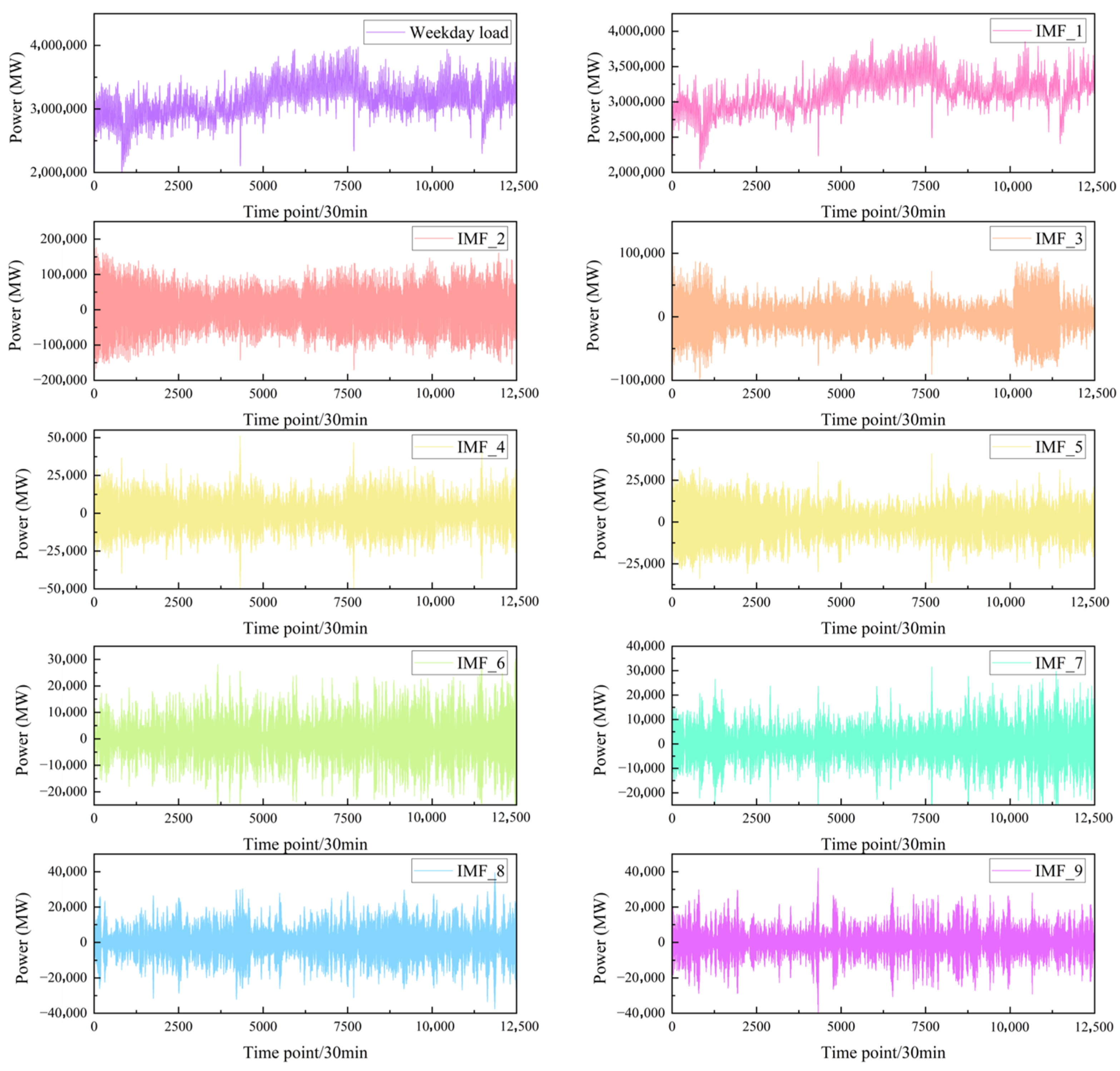
Taking the weekday dataset as an example, the specific decomposition results of VMD optimized by MCPO are shown in Figure 4.

From Figure 4, the optimized VMD uses MCPO to determine the optimal K–α. It effectively decomposes into 9 IMF components. IMF 1 has a relatively high frequency. It reflects high-frequency signal fluctuations. IMF 9 has a low frequency. It shows the basic trend. Each component has limited bandwidth. There is no obvious mode mixing. This verifies that parameter optimization improves decomposition quality. It provides clearer multi-frequency features for subsequent model input.

3.5. Ablation Experiment

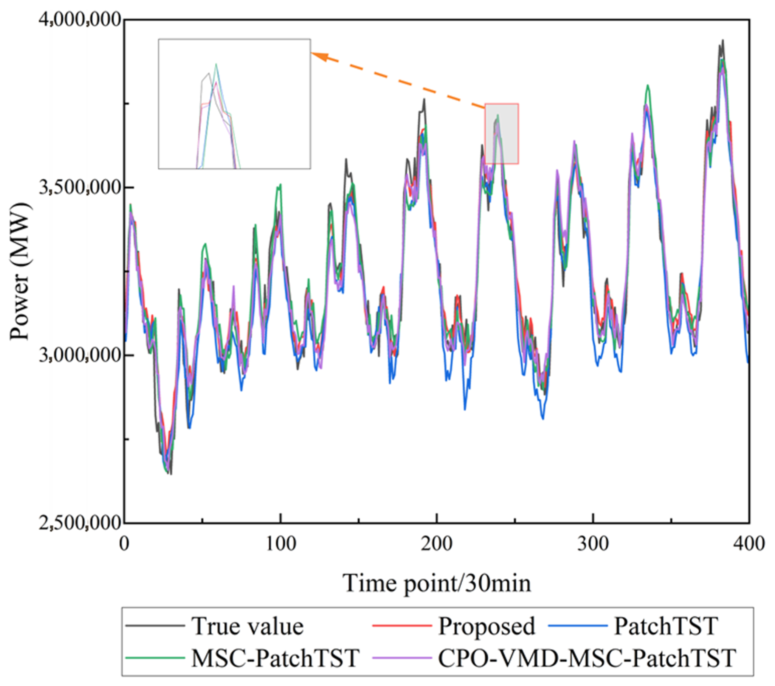
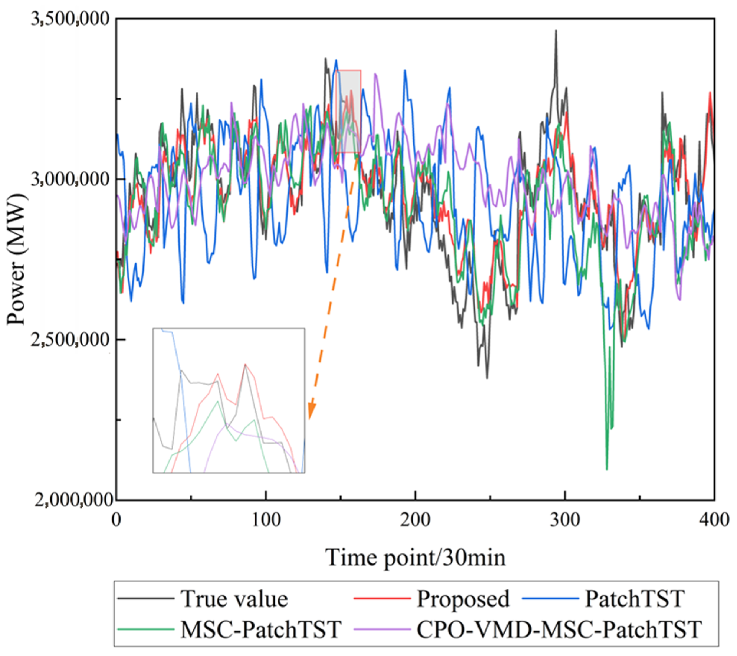
The results of the ablation study are presented in

Table 2. Ablation Experiment Prediction Metrics on User-Side Load Data.

Data Type	Method	RMSE	MAE	MAPE%
Weekdays	PatchTST	89,929.68	69,955.73	2.1973
	MSCPatchTST	76,526.31	58,820.48	1.8664
	CPO-VMD-MSCPatchTST	68,999.37	50,619.42	1.6174
	MCPO-VMD-MSCPatchTST	67,438.94	50,379.3	1.6001
	Proposed	59,131.17	44,954.44	1.4384
Saturdays	PatchTST	158,580.61	122,474.26	3.926
	MSCPatchTST	145,094.88	112,955.72	3.6334
	CPO-VMD-MSCPatchTST	127,526.27	96,752.75	3.1212
	MCPO-VMD-MSCPatchTST	126,446.16	95,918.71	3.0941
	Proposed	123,069.89	93,108.72	3.0026
Sundays	PatchTST	136,026.05	107,074.64	3.6329
	MSCPatchTST	111,315.49	86,603.41	2.9148
	CPO-VMD-MSCPatchTST	110,783.8	89,448.47	3.0025
	MCPO-VMD-MSCPatchTST	90,260.43	68,000.33	2.2815
	Proposed	86,655.03	64,351.65	2.2084

and Figure 5, Figure 6 and Figure 7. The experimental findings demonstrate that the proposed MCPO-VMD module, FDFE module, and MSC module each contribute to improved forecasting performance on user-side load data across weekdays, Saturdays, and Sundays during the period from 2 January 2024 to 17 March 2025.

Specifically, after incorporating the MSC module, the model is able to extract multi-scale features and adaptively fuse them, resulting in average reductions of 13.25%, 13.76%, and 13.77% in RMSE, MAE, and MAPE, respectively. This confirms the module’s effectiveness in capturing local and multi-scale information. In addition, the integration of the MCPO-VMD module allows the model to optimize the VMD process via the MCPO algorithm, significantly reducing data complexity and extracting multi-frequency characteristics. This improves the quality of the model input and achieves average reductions of 26.05%, 28.40%, and 28.52% in RMSE, MAE, and MAPE, respectively, demonstrating its enhanced ability to process non-stationary signals. Furthermore, with the addition of the FDFE module, the model can extract dominant and significant secondary frequency components in the frequency domain and enhance their key responses through an adaptive weighting mechanism. This leads to average improvements of 30.32%, 32.37%, and 31.84% in RMSE, MAE, and MAPE, respectively, validating the module’s capability in enhancing the perception of frequency-domain structural features. Overall, the proposed multi-dimensional CPO-VMD-MSC-PatchTST model, with the joint optimization of the CPO-VMD and MSC modules, significantly outperforms the baseline PatchTST. Compared to PatchTST, it achieves average reductions of 30.32%, 32.37%, and 31.84% in RMSE, MAE, and MAPE, respectively, confirming the effectiveness of the proposed modules in improving forecasting accuracy.

To validate the effectiveness of key components individually, ablation studies were conducted. First, to assess the optimization role of the customized fitness function in MCPO, “CPO-VMD-MSCPatchTST” was compared with “MCPO-VMD-MSCPatchTST.” The results show that the weekday RMSE decreased from 68,999.37 to 67,438.94, and on Sunday, the RMSE dropped from 110,783.8 to 90,260.43, with the MAPE% decreasing from 3.0025 to 2.2815. This indicates that the MCPO-based fitness function improves the accuracy of VMD parameter selection, thereby reducing prediction error.

Furthermore, to verify the value of the multi-scale convolution module, the baseline “PatchTST” model was compared with “MSCPatchTST,” which incorporates the module. Experimental data showed that the weekday RMSE decreased from 89,929.68 to 76,526.31, the Saturday MAPE% decreased from 3.926 to 3.6334, and the Sunday RMSE decreased from 136,026.05 to 111,315.49. This result demonstrates that the introduction of multi-size convolution kernels enhanced the model’s capability for extracting multi-scale load features.

From Figure 5, the proposed model is closer to the true value throughout the prediction period, especially in the high-fluctuation regions. Compared with PatchTST, MSC-PatchTST, and CPO-VMD-MSC-PatchTST, it shows smaller deviations, which is consistent with the lower error metrics in Table 2. Figure 6 presents a similar pattern. The proposed model can better capture the load variation characteristics on Saturdays. In the local enlarged area, its prediction curve fits the true value more closely, effectively reducing the overestimation or underestimation phenomena that occur in other comparative models. For Figure 7, the proposed model also demonstrates excellent prediction performance. Even in the regions with significant load fluctuations, it can follow the trend of the true load values well, further verifying the effectiveness of the integrated modules in improving the model’s adaptability to different load patterns on Sundays.

3.6. Comparative Experiment

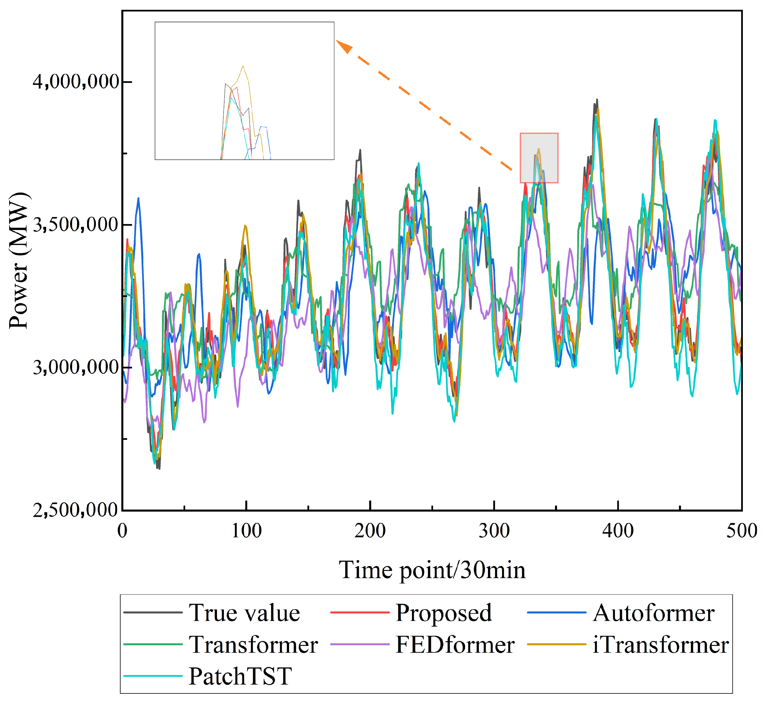
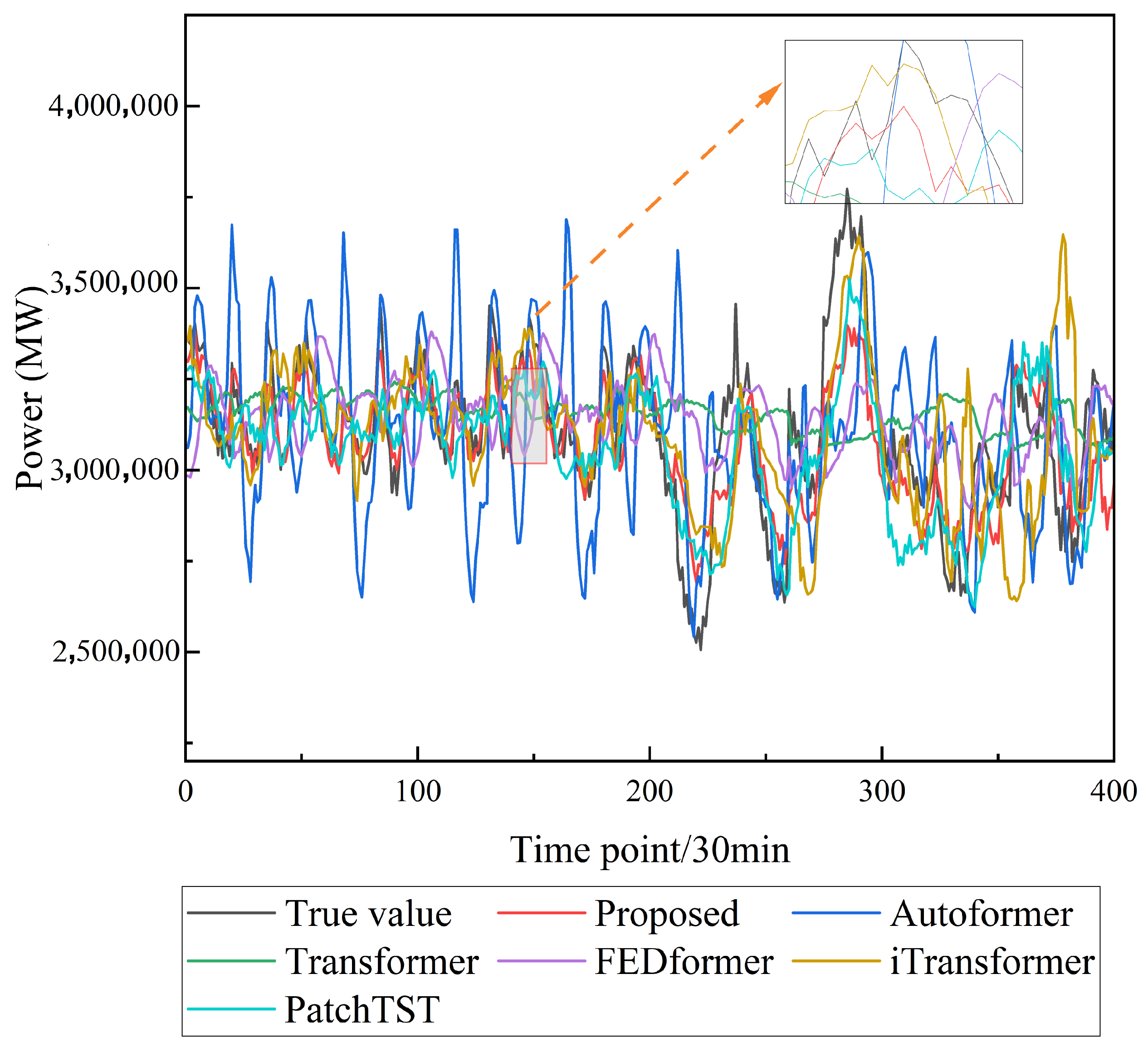
To evaluate the effectiveness of the proposed method in user-side load forecasting, several baseline models—including Autoformer, Transformer, FEDformer, iTransformer, and PatchTST—are selected for comparison. The forecasting performance of all models on user-side load data is summarized in

Table 3. Comparative Experiment 1: Prediction Metrics on User-Side Load Data.

Data Type	Method	RMSE	MAE	MAPE%
Weekdays	Autoformer	202,945.7	157,396.15	4.9929
	Transformer	188,512.8	150,230.16	4.7268
	FEDformer	221,169.5	172,782.76	5.372
	iTransformer	78,522.16	59,294.69	1.8536
	PatchTST	89,929.68	69,955.73	2.1973
	Proposed	76,526.31	58,820.48	1.8664
Saturdays	Autoformer	246,141.07	195,330.32	6.2523
	Transformer	238,694.39	180,513.21	5.9675
	FEDformer	228,628.75	181,450.29	5.9254
	iTransformer	204,594.55	144,689.18	4.7746
	PatchTST	158,580.61	122,474.26	3.926
	Proposed	145,094.88	112,955.72	3.6334
Sundays	Autoformer	272,625.66	222,147.36	7.6234
	Transformer	219,467.04	177,725.57	6.0307
	FEDformer	208,630.76	159,150.79	5.5775
	iTransformer	178,165.15	130,458.19	4.4611
	PatchTST	136,026.05	107,074.64	3.6329
	Proposed	111,315.49	86,603.41	2.9148

and Figure 8, Figure 9 and Figure 10. Experimental results show that the proposed MCPO-VMD-FDFE-MSCPatchTST model consistently outperforms all baseline models across the three datasets (weekdays, Saturdays, and Sundays). Compared to the baseline models, the proposed model achieves an overall RMSE reduction of 45.65% across the three user-side load forecasting tasks. Taking the weekday dataset as an example, the MCPO-VMD-FDFE-MSCPatchTST model achieves average reductions of 51.01%, 51.69%, and 51.24% in RMSE, MAE, and MAPE, respectively, compared to the other models. These results confirm the proposed model’s significant advantages and practical effectiveness in modeling non-stationary load sequences and improving forecasting accuracy.

The visualization in Figure 8 shows that the proposed model’s prediction curve has a higher degree of agreement with the true values over the entire forecast period, particularly in high-fluctuation intervals such as peak and valley loads. Compared to baseline models like Autoformer and Transformer, this model achieves a better fit, which is consistent with the quantitative error metrics in Table 3. This result indicates that the model is capable of capturing the high-frequency, multi-peak-valley fluctuation characteristics of weekday loads. From Figure 9, it can be seen that the proposed model’s prediction curve is able to follow the trend of the true values. At the locally magnified load mutation points, this model’s prediction deviation is smaller than that of other compared models. This suggests that the model adapts well to the unique load fluctuation patterns of Saturdays, thereby reducing overestimation or underestimation in the prediction results. As shown in Figure 10, when faced with scenarios of sharp drops or surges in Sunday loads, the proposed model’s predictions remain largely consistent with the trend of the true values. This reflects the model’s stable performance in handling complex, non-stationary Sunday load sequences and demonstrates its generalization ability across different scenarios.

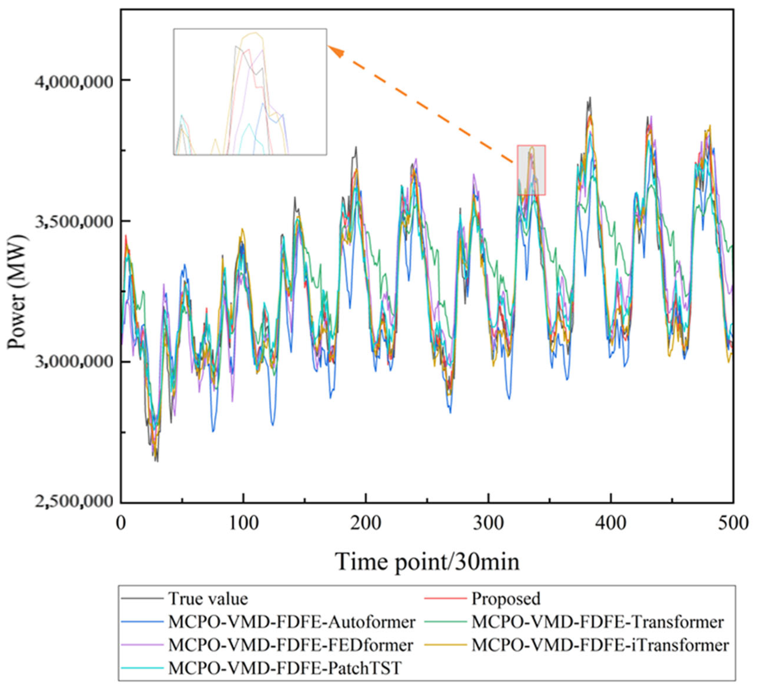
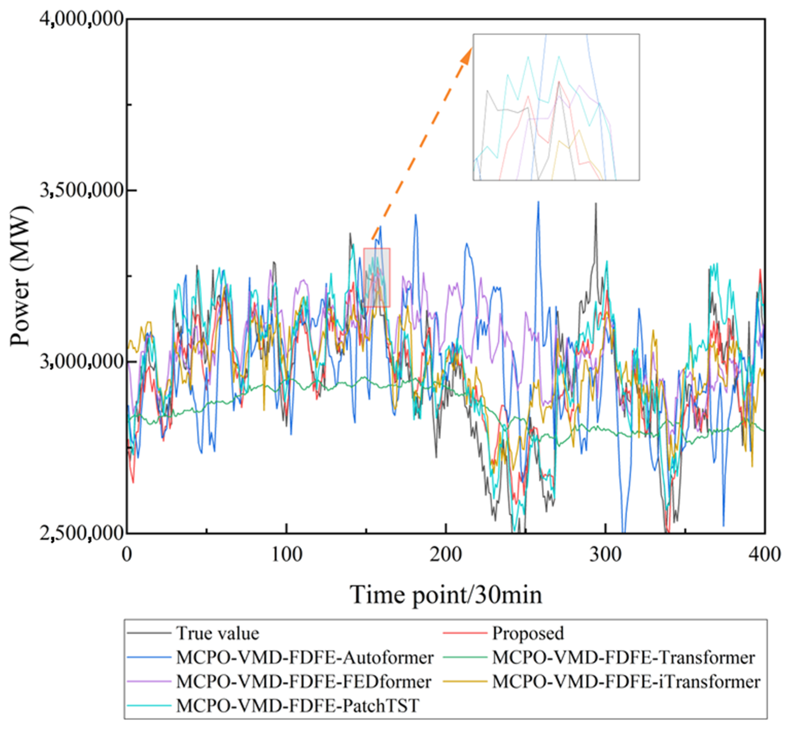
To further verify the effectiveness of the proposed integrated modeling strategy, the MCPO-VMD-FDFE decomposition-enhancement framework is embedded into five backbone models—Autoformer, Transformer, FEDformer, iTransformer, and PatchTST—for comparative experiments. The forecasting performance of each hybrid model on user-side load prediction tasks is presented in

Table 4. Comparative Experiment 2: Prediction Metrics on User-Side Load Data.

Data Type	Method	RMSE	MAE	MAPE%
Weekdays	MCPO-VMD-FDFE-Autoformer	155,956.6	116,683.01	3.7178
	MCPO-VMD-FDFE-Transformer	156,730.6	127,942.28	4.0373
	MCPO-VMD-FDFE-FEDformer	140,537.6	103,701.17	3.3195
	MCPO-VMD-FDFE-iTransformer	65,562.17	50,632.98	1.5981
	MCPO-VMD-FDFE-PatchTST	74,270.74	57,654.24	1.8427
	Proposed	59,131.17	44,954.44	1.4384
Saturdays	MCPO-VMD-FDFE-Autoformer	239,407.91	186,681.7	6.1231
	MCPO-VMD-FDFE-Transformer	220,768.05	170,794.68	5.5672
	MCPO-VMD-FDFE-FEDformer	204,852.45	152,448.84	5.0609
	MCPO-VMD-FDFE-iTransformer	184,007.49	133,593.04	4.4049
	MCPO-VMD-FDFE-PatchTST	136,738.68	103,215.95	3.3602
	Proposed	123,069.89	93,108.72	3.0026
Sundays	MCPO-VMD-FDFE-Autoformer	243,951.2	186,081.62	6.4431
	MCPO-VMD-FDFE-Transformer	209,132.61	171,928.29	5.7637
	MCPO-VMD-FDFE-FEDformer	200,642.97	149,461.14	5.2794
	MCPO-VMD-FDFE-iTransformer	139,269.59	110,671.9	3.8287
	MCPO-VMD-FDFE-PatchTST	91,299.71	74,078.26	2.5305
	Proposed	86,655.03	64,351.65	2.2084

and Figure 11, Figure 12 and Figure 13. The experimental results show that the proposed MCPO-VMD-FDFE-MSCPatchTST model consistently achieves superior performance across all three user-side load datasets: weekdays, Saturdays, and Sundays. Compared to the other hybrid models, it achieves an overall reduction of 46.25% in RMSE across the three datasets. Taking the weekday dataset as an example, the MCPO-VMD-FDFE-MSCPatchTST model outperforms all other models with average reductions of 49.98%, 50.68%, and 50.45% in RMSE, MAE, and MAPE, respectively. These results demonstrate the strong effectiveness and robustness of the proposed model in user-side load forecasting tasks.

From Figure 11, the proposed model aligns much closer with the true values throughout the entire prediction period, especially in high-fluctuation intervals with frequent load peaks and valleys. Its fitting degree surpasses that of hybrid models like MCPO-VMD-FDFE-Autoformer and MCPO-VMD-FDFE-Transformer. This clearly demonstrates the model’s ability to accurately fit the weekday load patterns and verifies its effectiveness in capturing high-frequency, multi-peak-valley fluctuation characteristics. From Figure 12, the prediction curve of the proposed model closely follows the changes in true values. In locally enlarged regions with load mutation points, it shows smaller deviations compared to other hybrid models. This strongly proves that the model can precisely adapt to the unique fluctuation patterns of Saturday loads arising from differences in work-rest schedules and electricity consumption habits, reducing over-prediction or under-prediction situations. From Figure 13, when facing extreme fluctuations of Sunday loads with scenarios of significant drops or sudden surges, the proposed model can still stably align with the trend of true values. This highlights the advantages of the integrated modules in handling complex, non-stationary Sunday load sequences and further supports the model’s generalization ability across multiple scenarios.

4. Conclusions

To address the limitations of poor adaptability in modal decomposition and insufficient frequency-domain feature representation in short-term user-side load forecasting tasks, this study proposes a novel forecasting method based on the MCPO-VMD-FDFE-MSCPatchTST framework. The effectiveness of the proposed method is verified through case studies, and the following conclusions are drawn:

(1)

This study proposes a parameter optimization method based on MCPO with a multi-dimensional fitness function, which overcomes the limitations of traditional empirical parameter selection to better match the multi-frequency characteristics of user-side load data. This method enables more effective optimization of key VMD parameters, and ablation studies show that its inclusion leads to average reductions of 26.05%, 28.40%, and 28.52% in RMSE, MAE, and MAPE, respectively, demonstrating its capability in handling non-stationary signals.

(2)

A frequency-domain feature enhancement (FDFE) module is designed to highlight key frequency components through adaptive thresholds and weighting strategies. This significantly improves the representational capacity of modal components. Ablation study results indicate that the inclusion of this module leads to average reductions of 30.32%, 32.37%, and 31.84% in RMSE, MAE, and MAPE, respectively, confirming its effectiveness in enhancing the model’s perception of frequency-domain structural features.

(3)

The integration of a multi-scale convolution module into the PatchTST model enables the collaborative extraction and adaptive fusion of both local and multi-scale features. This enhances the model’s ability to capture diverse patterns in user-side load data. Ablation study results show that this module contributes to average reductions of 26.05%, 28.40%, and 28.52% in RMSE, MAE, and MAPE, respectively.

(4)

The proposed method organically combines the MCPO-VMD decomposition, FDFE, and MSCPatchTST modules into a unified framework. This integrated approach achieves favorable forecasting performance across all three user-side load datasets (weekdays, Saturdays, and Sundays). Experimental results demonstrate that the proposed method consistently outperforms all comparison models, with an overall RMSE reduction of 45.65%, fully validating its effectiveness and stability in user-side load forecasting tasks.

(5)

Under the dataset and parameter settings used in this study, the complete workflow from training to prediction can be accomplished within approximately half an hour on a standard computing platform. This indicates that the proposed framework not only achieves high forecasting accuracy but also demonstrates satisfactory computational efficiency.

References

1. Wang, W.; Chen, Y.; Xiao, C.; Yang, Y.; Yao, J. Design of short-term load forecasting method considering user behavior. Electr. Power Syst. Res. 2024, 234, 110529. [Google Scholar] [CrossRef]
2. Zhao, W.; Mu, G.; Zhu, Y.; Xu, L.; Zhang, D.; Huang, H. Research on electric load forecasting and user benefit maximization under demand-side response. Int. J. Swarm Intell. Res. 2023, 14, 1–20. [Google Scholar] [CrossRef]
3. Liu, Y.B.; Wu, H.; Liu, T.J.; Yang, Z.Y.; Liu, J.Y.; Li, Q.H. User-Side Net Load Forecasting Algorithm Integrating Empirical Mode Decomposition and Deep Learning. Autom. Electr. Power Syst. 2021, 45, 57–64. [Google Scholar]
4. Yan, Q.; Lu, Z.; Liu, H.; He, X.; Zhang, X.; Guo, J. An improved feature-time Transformer encoder-Bi-LSTM for short-term forecasting of user-level integrated energy loads. Energy Build. 2023, 297, 113396. [Google Scholar] [CrossRef]
5. Wei, L.; Zhao, J. Hybrid CNN-Multivariate LSTM Model for Accurate Short-Term Electricity Price Forecasting and Energy System Optimization. J. Circuit Syst. Comput. 2025, 34, 2550198. [Google Scholar] [CrossRef]
6. Yuqi, J.; An, A.; Lu, Z.; Ping, H.; Xiaomei, L. Short-term load forecasting based on temporal importance analysis and feature extraction. Electr. Power Syst. Res. 2025, 244, 111551. [Google Scholar] [CrossRef]
7. Li, Y.; Wang, H.; Huang, X.; Hao, J.; Lei, W.; Wang, Q. Short-term power load forecasting in distribution networks considering human comfort level. Front. Energy Res. 2025, 13, 1514755. [Google Scholar] [CrossRef]
8. Ahmad, A.; Xiao, X.; Mo, H.; Dong, D. TFTformer: A novel transformer based model for short-term load forecasting. Int. J. Electr. Power Energy Syst. 2025, 166, 110549. [Google Scholar] [CrossRef]
9. Liu, W.; Li, J. Short-term power load forecasting based on genetic algorithm improved VMD-BP. Int. J. Intell. Inf. Technol. 2025, 21, 1–18. [Google Scholar] [CrossRef]
10. Zhang, W.; Zhong, A.; Duan, K.; Shao, L. Ultra-short-term user-level load forecasting based on multi-scale component feature learning. Power Syst. Technol. 2024, 48, 2584–2592. [Google Scholar]
11. Cao, H.Z.; Wei, B.; Gao, C.; Wu, J.K.; Lei, Z.; Sui, Y.; Chen, Y.B. Short-Term Electric Load Forecasting Method Based on Deep Belief Network. New Type Power Syst. 2025, 3, 111–124. [Google Scholar]
12. Chen, C.; Ma, H.R.; Chen, L.J.; Ren, B.W.; Jin, C.; Zhang, T.Y. Multi-Step Short-Term Load Forecasting Method Based on User Group Segmentation. High Volt. Eng. 2023, 49, 4213–4222. [Google Scholar]
13. Moudgil, V.; Sadiq, R.; Brar, J.; Hewage, K. Dual-channel encoded bidirectional LSTM for multi-building short-term load forecasting. J. Clean. Prod. 2025, 486, 144555. [Google Scholar] [CrossRef]
14. Liu, F.; Wang, X.; Zhao, T.; Zhang, L.; Jiang, M.; Zhang, F. Novel short-term low-voltage load forecasting method based on residual stacking frequency attention network. Electr. Power Syst. Res. 2024, 233, 110534. [Google Scholar] [CrossRef]
15. Zhang, Q.; Chen, J.; Xiao, G.; He, S.; Deng, K. TransformGraph: A novel short-term electricity net load forecasting model. Energy Rep. 2023, 9, 2705–2717. [Google Scholar] [CrossRef]
16. Yazici, I.; Beyca, O.F.; Delen, D. Deep-learning-based short-term electricity load forecasting: A real case application. Eng. Appl. Artif. Intell. 2022, 109, 104645. [Google Scholar] [CrossRef]
17. Zhuang, H.; Guo, X.; Shan, D.; Tian, X.; Hou, T. Short-term power load forecasting model based on optimized VMD-BILSTM. In Proceedings of the 2023 8th Asia Conference on Power and Electrical Engineering (ACPEE), Tianjin, China, 14–16 April 2023; pp. 2029–2033. [Google Scholar] [CrossRef]
18. Zhang, Z.; Hong, W.C. Application of variational mode decomposition and chaotic grey wolf optimizer with support vector regression for forecasting electric loads. Knowl. Based Syst. 2021, 228, 107297. [Google Scholar] [CrossRef]
19. Yang, W.; Shi, J.; Li, S.; Song, Z.; Zhang, Z.; Chen, Z. A combined deep learning load forecasting model of single household resident user considering multi-time scale electricity consumption behavior. Appl. Energy 2022, 307, 118197. [Google Scholar] [CrossRef]
20. Tang, Q.F.; Liu, N.; Zhang, J.H.; Yu, Z.Z.; Zhang, Q.X.; Lei, J.Y. Short-Term Load Forecasting Method for User-Side Microgrids Based on EMD-KELM-EKF and Parameter Optimization. Power Syst. Technol. 2014, 38, 2691–2699. [Google Scholar]
21. Zhou, M.; Yu, J.; Wang, M.; Quan, W.; Bian, C. Research on the combined forecasting model of cooling load based on IVMD-WOA-LSSVM. Energy Build. 2024, 317, 114339. [Google Scholar] [CrossRef]
22. Li, H.; Tang, Y.; Liu, D. A CrossInformer model based on dual-layer decomposition and interpretability for short-term electricity load forecasting. Alex. Eng. J. 2025, 129, 117–127. [Google Scholar] [CrossRef]
23. Cui, X.; Zhang, X.; Niu, D. A new framework for ultra-short-term electricity load forecasting model using IVMD–SGMD two–layer decomposition and INGO–BiLSTM–TPA–TCN. Appl. Soft Comput. 2024, 167, 112311. [Google Scholar] [CrossRef]
Figure 1. Overall framework.
Electronics 14 03611 g001
Figure 2. Flowchart of CPO.
Electronics 14 03611 g002
Figure 3. MSCPatchTST Framework. (a) Overall structure of MSCPatchTST. (b) Schematic diagram of transformer structure.
Electronics 14 03611 g003
Figure 4. VMD Decomposition Results.
Electronics 14 03611 g004
Figure 5. Ablation Study on Weekdays Load Data.
Electronics 14 03611 g005
Figure 6. Ablation Study on Saturdays Load Data.
Electronics 14 03611 g006
Figure 7. Ablation Study on Sundays Load Data.
Electronics 14 03611 g007
Figure 8. Comparison Experiment a on Weekdays Load Data.
Electronics 14 03611 g008
Figure 9. Comparison Experiment a on Saturdays Load Data.
Electronics 14 03611 g009
Figure 10. Comparison Experiment a on Sundays Load Data.
Electronics 14 03611 g010
Figure 11. Comparison Experiment b on Weekdays Load Data.
Electronics 14 03611 g011
Figure 12. Comparison Experiment b on Saturdays Load Data.
Electronics 14 03611 g012
Figure 13. Comparison Experiment b on Sundays Load Data.
Electronics 14 03611 g013