Article

Short-Term Photovoltaic Power Prediction Model Based on Variational Modal Decomposition and Improved RIME Optimization Algorithm

1
School of Electrical Engineering, Guangxi University, Nanning 530004, China
2
China Resources New Energy (Tengxian) Co., Ltd., Wuzhou 543300, China
*
Author to whom correspondence should be addressed.
Electronics 2025, 14(18), 3612; https://doi.org/10.3390/electronics14183612
Submission received: 11 August 2025 / Revised: 5 September 2025 / Accepted: 10 September 2025 / Published: 11 September 2025

Abstract

Photovoltaic (PV) power generation is highly stochastic and volatile, a trait that presents a notable challenge to the prediction accuracy of distributed PV systems. To address this challenge, this study proposes a short-term photovoltaic power prediction strategy that integrates variational modal decomposition (VMD) for feature extraction with an improved RIME (IRIME) optimization algorithm for parameter optimization. Firstly, the raw PV power data are split into several intrinsic mode functions (IMFs) using VMD. The decomposed IMFs are reconstructed by using the sample entropy (SE) method, and a new subsequence with enhanced features is obtained. Secondly, a bidirectional gated recurrent unit (BIGRU) prediction model is established, and its structural parameters are optimized by the IRIME algorithm. Finally, the prediction results of each subsequence are summarized to obtain the final prediction value. Information from a centralized PV power station located in southern China is employed to verify the suggested prediction model. Experimental findings indicate that in comparison with other models, the proposed model achieves the smallest PV power prediction error; the mean absolute error (MAE), mean absolute percentage error (MAPE), and root mean square error (RMSE) of the proposed model are reduced at least by 21.95%, 3.03%, and 12.33%, respectively. The coefficient of determination (R2) is increased at least by 10.56‰. The method presented in this research is capable of improving prediction accuracy efficiently and holds specific engineering practicality.

1. Introduction

As the global economy advances and fossil fuels are depleted, renewable energy sources (RES) assume a growingly critical role in improving the energy structure, preserving the ecological environment, and driving economic growth and social progress [1]. Vigorously developing renewable energy has become a global consensus. Solar energy is an ideal green energy source with the advantages of being pollution-free and sustainable. Solar photovoltaic power generation’s installed capacity is on the rise annually. Per the “2025 Renewable Energy Capacity Statistics Report” released by the International Renewable Energy Agency (IRENA), the global growth rate of new solar power capacity in 2024 stood at 32.2%, with the newly added capacity hitting 451.9 GW—representing over 70% of the world’s total new renewable energy capacity [2]. Nevertheless, photovoltaic power generation is directly influenced by solar irradiance, ambient temperature, seasonal shifts, and other meteorological factors, exhibiting marked randomness and fluctuating traits [3,4]. Large-scale grid-connected PV power will present significant challenges to the stability, reliability, and power balance of the power system [5,6]. Therefore, accurate prediction of PV power generation is vital to the safe and stable operation of photovoltaic power generation systems. Effective prediction technologies can enhance the accuracy of optimal PV power generation forecasting, thereby ensuring the system’s safe and stable operation [7,8].
At present, prediction methods for PV power generation mainly include physical methods, statistical methods, and machine learning models [9]. Physical methods rely on local cloud map data and the operating mechanism of PV modules to determine the output power of a PV station, which is a complex process and highly dependent on geographic and weather forecast information [10]. The neural network model embedded with physical formulas for PV power generation enhances prediction robustness under extreme weather conditions. However, the construction of the involved physical model is relatively difficult [11]. Statistical models reduce computational complexity by mining information from historical data to build mapping models without considering the PV conversion process [12]. Commonly used statistical models include linear regression models, principal component regression (PCR) [13], Markov chain (MC) [14], and autoregressive integral moving average (ARIMA) [15]. However, statistical models are limited in their ability to capture nonlinear data, thus the prediction accuracy is not high. In recent years, with the rapid development of machine learning techniques, their application in the field of PV power prediction has become increasingly widespread. Machine learning prediction techniques may be divided into shallow learning models and deep learning models. Shallow learning models include artificial neural network (ANN) [16], random forest (RF) [17], support vector machine (SVM) [18], and extreme learning machine (ELM) [19]. However, these models still face problems such as overfitting, high computational cost, and complex feature engineering. In order to extract complex nonlinear features of data more efficiently and perform more accurate time series prediction, deep learning (DL) models such as recurrent neural networks (RNN), long short-term memory networks (LSTM), and gated recurrent units (GRU) have been widely used in this field. These deep learning models have proven to be powerful forecasting tools [20].
The LSTM and GRU algorithms are employed for PV power prediction under varying weather conditions. The findings indicate that deep learning models outperform statistical methods and machine learning models in terms of prediction accuracy [21,22]. The model integrating spatiotemporal feature interaction and an Attention mechanism improves prediction accuracy by focusing on key meteorological features and temporal nodes. While it demonstrates a strong ability to capture long-sequence dependencies, it exhibits high computational complexity [23]. The hybrid Transformer–LSTM model is applied to short-term photovoltaic (PV) power forecasting. Although it possesses good generalization ability, the Transformer architecture typically has high data requirements and is limited by the need for a large number of samples for training [24]. But they only consider one-way data information and ignore the influence of reverse data information, resulting in low prediction accuracy when processing time series data. A study has proposed a multivariate input prediction method based on the GRU model. The effectiveness of the proposed method is demonstrated by its better prediction accuracy performance when compared to traditional RNN, BP neural networks, and radial basis function (RBF) models. This enhancement in prediction accuracy is attributed to the incorporation of environmental features, including temperature, humidity, and solar radiation intensity, as input parameters [25]. To mitigate the interference of data noise on PV power prediction, it is essential to reduce signal non-stationarity and extract its intrinsic features via data decomposition methods. A short-term PV power generation interval prediction model was established using empirical modal decomposition (EMD) and correlation vector machine (RVM), which improved the PV prediction accuracy [26,27], while EMD is easily affected by end effect, leading to unstable decomposition results, and reduces the prediction accuracy. Researchers have proposed a method for predicting future photovoltaic power generation that combines EEMD and BIGRU [28]. This method effectively addresses the modal overlap and endpoint effects issues inherent in traditional EMD algorithms. However, the EEMD algorithm is sensitive to high-frequency noise and introduces white noise during the decomposition process. Therefore, it is necessary to average the results of multiple decompositions to eliminate the noise effect. This process not only raises the computational complexity of the algorithm but also lowers computational efficiency [29]. In the process of signal decomposition, VMD exhibits stronger noise suppression capability, and when addressing time series problems, it achieves a better decomposition effect than EMD and EEMD [30]. Through VMD, the PV power sequence is split into several sub-modules; a power prediction model constructed with these sub-module sequences can efficiently capture the nonlinear characteristics of photovoltaic power sequences and boost the accuracy of forecasting [31,32]. Yet, the above-mentioned studies disregard the characteristics of data decomposition: they apply the same prediction method to all decomposed subsequences, failing to account for the frequency-dependent properties of each subsequence and the effect of deep learning network parameters on the accuracy of predictions. This neglect of the potential differences and significance of different frequency components in prediction may result in inaccurate or unstable forecasting results. At the same time, PV power prediction models involve a great many hyperparameters, and finding suitable values through manual tuning proves challenging. This is not only time-consuming and laborious, but also often struggles to achieve optimal prediction results, as different hyperparameter combinations may yield significantly divergent forecasting outcomes [33,34]. A number of studies have previously implemented the RIME algorithm in the context of optimizing I-beam structural design, the AGC process of photovoltaic thermal power generation systems, and the optimization and reconstruction of thermoelectric generator arrays within the scope of actual engineering projects. The findings suggest that RIME is a robust and competitive algorithm that exhibits notable applicability and effectiveness in practical engineering applications [35,36]. It is noteworthy that while the RIME optimization algorithm demonstrates remarkable global search capabilities and expeditious convergence speeds in specific contexts, extant studies have yet to substantiate its equivalent optimization performance in intricate domains such as power time series prediction. When confronted with optimization tasks in complex real-world scenarios, such as photovoltaic power generation, the RIME algorithm may encounter challenges related to slow convergence speed. This is particularly evident when addressing multimodal problems, where the algorithm tends to fall into local optima and thus finds it difficult to reach the global optimal solution. The summary of novel photovoltaic power generation methods is shown in Table 1.
(a)
To address the non-stationarity and noise interference problems of PV power sequences, VMD is employed to decompose the original PV power sequence into multiple IMFs. Subsequently, SE is used for mode screening and reconstruction: the IMFs are divided into three groups (high-frequency, medium-frequency, and low-frequency), redundant noise modes are eliminated, and valid feature components are retained. This approach not only reduces data complexity but also avoids the end effect and mode-mixing problems associated with traditional decomposition methods.
(b)
To tackle the shortcomings of the traditional RIME algorithm—such as its tendency to fall into local optima and exhibit decreased convergence speed in PV power forecasting or high-dimensional nonlinear time series tasks—an original improvement is proposed to develop IRIME. On the one hand, an adaptive weight factor based on population diversity feedback and iteration progress coefficient is introduced to dynamically balance the algorithm’s global exploration and local exploitation capabilities. On the other hand, the cross-optimization search strategy (COSS) is integrated, and a crossover probability assignment rule based on individual fitness is designed to enhance the accuracy of hyperparameter optimization.
Table 1. Summary of novel approaches to PV power.
ReferencePrediction MethodAdvantageLimitation
[10,11]Modeling based on cloud and physical mechanismsGood robustness under extreme weatherThe model is complex and strongly dependent on geography
[13,14,15]Linear regression, ARIMA, PCR, MarkovLow computational complexityCannot capture the nonlinearity; the accuracy is not high
[16,17,18,19]ANN, RF, SVM, ELMThe implementation process is simpleThe model is easy to overfit, so complex feature engineering should be incorporated
[20,21,22]RNN, LSTM, GRUThe accuracy is better than the statistical and shallow modelsIgnoring the reverse information, the accuracy is still insufficient
[23]GRU, AttentionLong-sequence dependencies capture wellHigh computational complexity
[24]Transformer, LSTMStrong generalization abilityIt requires a large number of data samples to train
[26,27]EMD, RVMReduce noise interferenceAffected by the backdoor effect; decomposition is unstable
[28]EEMD, BIGRUMitigating modal aliasingIntroduces white noise; sensitive to high-frequency noise
[30,31,32]VMDThe decomposition effect is better than EMD/EEMDIgnores the differences in frequency characteristics of the subsequence
[35,36]RIME algorithmSome engineering application scenarios are highly robustIt has not been verified in the field of power timing prediction. When dealing with high-dimensional nonlinear problems such as photovoltaic power, it is easy to fall into local optimization, and the convergence speed decreases
The structure of this paper is as follows. Section 2 details the mathematical methods for VMD and SE data processing. Section 3 focuses on the improvement strategies of the RIME algorithm. Section 4 presents the experimental results of the proposed method and compares its prediction results with those of other existing prediction methods. Section 5 provides conclusions, including a summary of the work and future prospects.

2. Data Decomposition Reconstruction Methods

2.1. Variational Modal Decomposition

VMD refers to a signal processing technique that incorporates Wiener filtering, Hilbert transform, and epistatic demodulation to achieve non-recursive variational signal decomposition. This method exhibits significant advantages in processing time series data featuring strong nonlinearity and high complexity, and can effectively mitigate data instability [37,38]. The process is as follows:
Signal demodulation is performed using the Gaussian smoothness criterion and gradient-squared criterion, and its L2 norm is computed to acquire the bandwidth of each decomposed mode. The decomposed modes are amplitude–frequency signals. The variationally constrained model is shown as follows:
min u k ω k k = 1 K t δ ( t ) + j π t u k ( t ) e j w k t 2 2 s . t . k = 1 K u k = f ( t )
where K is the number of modes, t is the partial derivative operator, u k and ω k are the set of decomposed subsequences and center frequencies, respectively, δ t is the Dirac function, and ∗ denotes convolution.
To obtain the optimal solution for the aforementioned constrained variational model, a quadratic penalty factor α and a Lagrange multiplier λ ( t ) are introduced. Hence, the constrained variational problem may be converted into an unconstrained one, and the Lagrange function can be formulated as
L u k , ω k , λ = α k = 1 K t δ ( t ) + j π t u k ( t ) e j w k t 2 2 + f ( t ) u k ( t ) 2 2 + [ λ ( t ) , f ( t ) k = 1 K u k ( t ) ]
The “saddle point” of the Lagrangian function are used to the target value of the iterative update:
u ^ k n + 1 ( ω ) = f ^ ( ω ) k = 1 K u ^ k n + 1 ( ω ) k = 1 K u ^ k n ( ω ) + λ ^ ( ω ) 2 1 + 2 α ( ω ω k n ) 2
ω k n + 1 = 0 ω u ^ k n + 1 ( ω ) 2 d ω 0 u ^ k n + 1 ( ω ) 2 d ω
λ ^ k n + 1 ( ω ) = λ ^ k n ( ω ) + τ ( f ^ ( ω ) k = 1 K u ^ k n + 1 ( ω ) )
where τ is the fidelity coefficient.
It must satisfy the convergence conditions:
k = 1 K u ^ k n + 1 u ^ k n 2 2 u ^ k n 2 2 < ϕ
where K is the number of modes and ϕ is the convergence factor.
To mitigate the influence of PV data noise on forecasting outcomes, parameter settings are as follows: the number of modes K = 8, the penalty factor α = 2000 , the fidelity coefficient τ = 10 3 , and the convergence coefficient ϕ = 10−7.

2.2. Sample Entropy

SE, an improved algorithm built on approximate entropy, is capable of quantifying time series complexity more accurately. In the context of time series analysis, the larger the SE value, the higher the complexity of such time series [39,40]. For a time series X = x 1 , x 2 , x n 1 , x n that includes n time points, the steps for calculating SE are outlined as follows:
1.
Construct an m-dimensional vector from the time series X:
X i = x i , x i + 1 , , x i + m 1
where m is a fixed positive integer, i = 1 , 2 , , n m + 1 .
2.
With respect to any two different vectors X i and X j , the maximum absolute value of their difference is determined as follows:
R max ( X i , X j ) = max x i + k x j + k k { 0 , 1 , 2 , , m 1 }
where R max ( X i , X j ) is equal to the infinite paradigm X i X j .
3.
For a given positive threshold and time series vector X i , the cardinal number of the set of { X j R max ( X i , X j ) < α , i j } is denoted as B i . The ratio of B i to Nm can be expressed by
B i m ( α ) B i N m
4.
Calculate the arithmetic mean of the results obtained from (9):
B m ( α ) = 1 N m + 1 i = 1 N m + 1 B i m ( α )
5.
The sample entropy of the original sequence X is
S a m p E n ( m , α ) = lim N ln B m + 1 ( α ) B m ( α )
In order to balance the accuracy and efficiency of the calculation, the number of dimensions m = 2 is taken in this paper.

3. Combinatorial Predictive Model

3.1. The Bidirectional Gated Recurrent Unit

BIGRU consists of a forward GRU and a reverse GRU. It can make the neural network able to simultaneously refer to the information of the previous texts, significantly improving the network’s learning ability. The network structure of BIGRU is shown in Figure 1.
The output values of BIGRU are shown below:
h t = G R U ( x t , h t 1 )
h t = w t h t + w t h t + b t
where x t is the hidden layer state at moment t, h t and h t are the outputs of the forward and reverse hidden layers at moment t, respectively; w t and w t denote the weights of the corresponding BIGRU forward hidden layer h t and reverse hidden layer h t at moment t, respectively; and b t denotes the bias.

3.2. IRIME Algorithm

As an intelligent optimization algorithm, RIME is formed by integrating the soft-freezing search strategy, hard-freezing puncturing mechanism, and greedy selection strategy, and its search principle process can be as follows [41].
The fog population consists of n fog agents, and the fog mass particles x i j are directly represented by R, which is shown as follows:
R = x 11 x 12 x 1 j x 21 x 22 x 2 j x i 1 x i 2 x i j , R = P 1 P 2 P i , P i = [ x i 1 , x i 2 , , x i j ]
Each particle’s position can be represented as
R i j n e w = R b e s t , j + r 1 cos θ β ( h ( U b i j L b i j ) + L b i j ) , r 2 < E
where R i j n e w denotes the updated new position of the particle; i and j represent the i-th particle and the j-th particle, respectively; U b i j and L b i j stand for the upper and lower boundaries of the search space, respectively; R b e s t , j indicates the j-th particle of the best particle; r 1 denotes a random ranging from −1 to 1; β is the environmental factor; and h and r 2 are both a random number in (0, 1).
θ = t π 10 T
β = 1 w t T / w
E = t / T
r 3 < F n o r m r ( f ( S i ) )
where w represents the convergence factor, t and T indicate the current number of iterations and the total number of iterations, respectively. r 3 denotes a random number between (−1, 1), F n o r m r ( f ( S i ) ) denotes the normalized value of the fitness of the i-th search agent, and r 3 bears a close relation to the normalized value of the i-th search agent’s fitness.
The RIME algorithm overly relies on finding the best individual position, which reduces the efficiency of population search and increases the probability of local optima. It cannot maintain a balance between global search and local utilization, which may lead to local search getting stuck in local optima and missing out on the global optimum. Therefore, the RIME algorithm is improved from the following two aspects.
  • Adaptive weighting factors w
In the RIME algorithm, w is used to control the stepping function. This factor exerts an influence on the local as well as global search performance of the algorithm. Thus, by nonlinearly changing the convergence factor w to balance the search efficiency of the algorithm, the optimization performance can be improved. The improved w is
W = 2 λ e w t T 2
λ = r a n d sin π t T + cos ( t T )
where W is the improved convergence factor, λ is the dynamic perturbation factor.
2.
Cross-optimization search strategy
Cross-optimization search strategy (COSS) is composed of two interacting search operators: horizontal crossover and vertical crossover. This distinctive crossover method serves a key function in preserving population diversity and assisting the stagnant dimension in escaping local minima, thereby enabling effective tackling of high-dimensional, non-convex optimization problems [42].
The expression for the horizontal crossover operation of the COSS algorithm is
M s h c i , d = r 1 X i , d + 1 r 1 X j , d                                         + c 1 X i , d X j , d
M s h c j , d = r 2 X j , d + 1 r 2 X i , d                                         + c 2 X j , d X i , d
where r1 and r2 are random numbers in [0, 1], c 1 and c 2 are random numbers in [−1, 1], M s h c ( i , d ) and M s h c ( j , d ) denote the next generation individuals obtained from the previous generation individuals X ( i , d ) and X ( j , d ) after horizontal crossover in the d-th dimension, respectively.
Vertical crossover denotes the crossover operation between all particles in two distinct dimensions. When the d1-th and d2-th dimensions of particle X ( i ) are subject to crossover, this results in
M s v c i , d 1 = r X i , d 1 + 1 r X i , d 2
where M s v c ( i , d 1 ) is the previous generation X ( i , d 1 ) in the d1-th dimension by longitudinal crossover to achieve the next generation of individuals, r represents a random number with a uniform distribution in [0, 1], M denotes the population size, D stands for the total particle dimension count, i is an integer of [1, M], and both d1 and d2 are integers of [1, D].
In this paper, a cross-optimization search strategy has been successfully and innovatively integrated into the RIME algorithm, which is used to optimize the position R i j n e w of the updated particle. In each evolutionary iteration, two new individuals of COSS particles can be obtained from (23)–(25), M s h c and M s v c . Then, the M s h c and M s v c are compared with the current X(i) and X(j). The individuals with low fitness are eliminated, and the individual with the best fitness is retained. This competitive mechanism guarantees that the RIME algorithm search consistently remains within the historically optimal population, further balancing resource allocation between global and local search. Consequently, the solution’s accuracy and convergence speed are enhanced.

3.3. Prediction Model Based on VMD-SE-IRIME-BIGRU
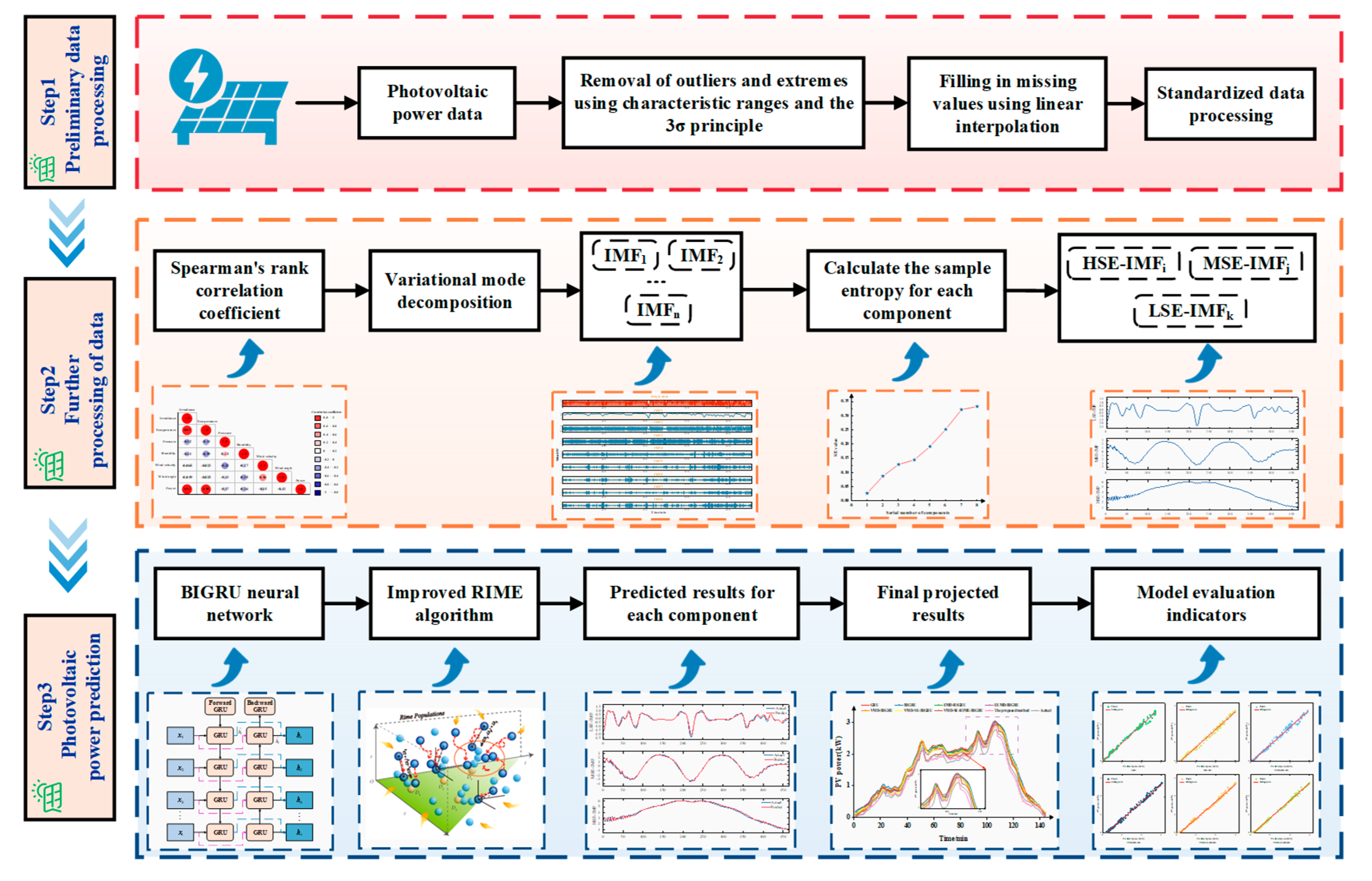
The process of the proposed short-term PV power prediction modeling approach is presented in Figure 2. The implementation steps are specified as follows:
Step 1: Remove as well as supplement the outliers in historical data on PV generation to maintain the integrity of this dataset. At the same time, perform normalization on different characteristic variables.
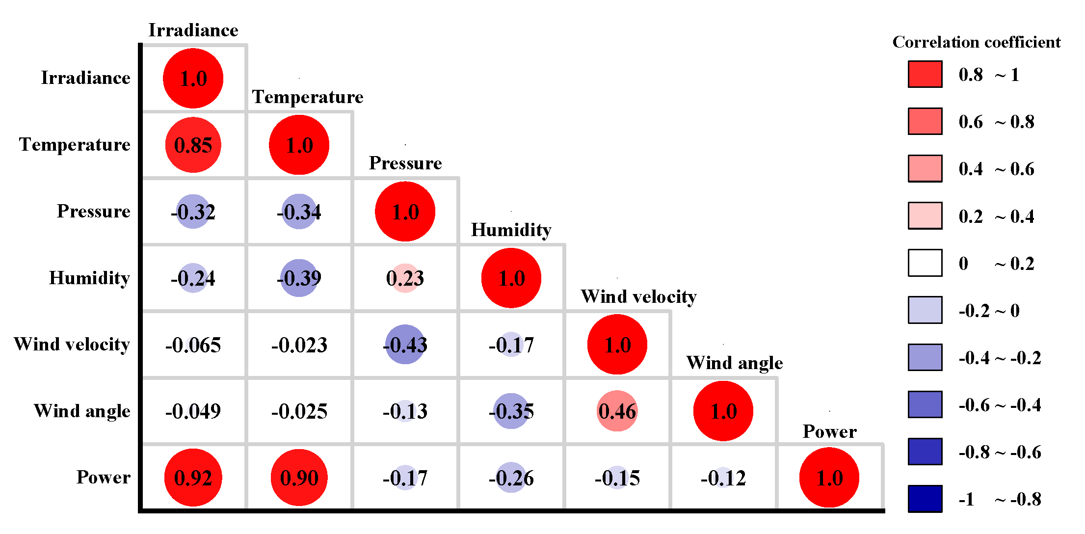
Step 2: Utilize Spearman correlation coefficient analysis to select meteorological factors exhibiting high correlation with photovoltaic power. Among these, the absolute value of Spearman directly mirrors the extent of correlation between the meteorological factor and PV power.
Step 3: The time series signal of historical photovoltaic power is decomposed using the variational modal decomposition technique. The independent mode function (IMFs) components and sample entropy are calculated, and the reconstruct is made based on the entropy value of each component.
Step 4: Initialize and configure the IRIME algorithm’s parameters, encompassing the maximum number of iterations, population size, optimal dimension, fog parameter, and search space boundary.
Step 5: Construct the BIGRU network model. Subject hidden layer parameters such as number of neurons, learning rate, and maximum training rounds to optimization. Set the value scope of optimized parameters and map the optimized parameters of the BIGRU network to the IRIME algorithm’s initial positions.
Step 6: The fitness value of the IRIME algorithm in the initial stage is calculated. The nonlinear weight factor is acquired to control the search function. The stepped soft fog search and hard fog puncture mechanism with positive greedy selection mechanism strategy are adopted to update the population; thus, the effective information between individuals is exchanged. In addition, crosswise and longitudinal crossover is used in the search process to save the best solution and exclude the bad solutions. Next, compare the current result with the historical best values to judge whether the best solution has been found or the maximum number of iterations has been achieved. If this condition is met, stop the iteration procedure; otherwise, continue the searching process.
Step 7: The optimal solution from IRIME optimization is transformed into the optimal parameter configuration of the BIGRU network. Training and prediction for the optimized hybrid model are performed using the example dataset. The ultimate prediction outcomes of the model are derived through addition and inverse normalization of the predicted values from all reconstructed components.
Step 8: Evaluation including MAE, RMSE, MAPE, and R2 are employed to comprehensively assess the predictive performance of different models.
Figure 2. Framework of the proposed photovoltaic power prediction model.
Electronics 14 03612 g002

4. Example Analysis

4.1. Data Sources

The dataset utilized in this paper originates from a PV power plant in southern China, encompassing historical time series of PV power generation, temperature, humidity, solar radiation intensity, wind speed, and wind direction. All computational cost tests in this paper are based on a unified hardware environment, with an Intel Core i5-10600K CPU (Intel, Santa Clara, CA, USA), 16 GB DDR4 memory (Kingston, Fountain Valley, CA, USA), the Windows 10 operating system, and the Python 3.9 + TensorFlow 2.8 programming framework. The collected dataset includes 120 days with a sampling period of 5 min, which has 34,560 samples. The data are divided into the training set, validation set, and test set in the ratio of 7:2:1. Spearman correlation coefficient ρ is employed to analyze the data’s correlation. If and only if ρ 0.8 , the correlation of data is highly correlated. The data correlation heat map is shown in Figure 3. As shown in Figure 3, the Spearman correlation coefficient ρ of radiation intensity and temperature is 0.90 and 0.92, respectively. Therefore, radiation intensity and temperature are selected as input signals in this paper.

4.2. Data Preprocessing

4.2.1. Data Missing Value Processing

For missing data, this paper adopts the k-nearest neighbor method for imputation as follows:
X n = X n k + + X n 1 + X n + 1 + + X n + k 2 k
where X n represents the missing data, X n k and X n + k represent the data before and after the k-th missing data, respectively.

4.2.2. Detection and Processing of Data Outliers

The 3 σ criterion is commonly used to identify outliers in a dataset. Its basic idea is to assume that the data to be tested contains only random errors; then, the standard deviation is calculated to determine the rejection interval. Residuals exceeding this interval are regarded as gross errors and must be rejected. Suppose there is a sample of n data points [X1, X2, …, Xn]; then, the standard deviation σ can be calculated as follows:
σ = n = 1 N ( X ¯ X n ) 2 N
| X V | = | X ¯ X n | > 3 σ
where X ¯ is the average value of the sample data, and X v can be regarded as abnormal data when it meets Formula (28).

4.2.3. Data Standardization

This paper uses the Min–Max normalization method to map the feature values of photovoltaic power and meteorological data to the interval [0, 1]. The calculations for normalization and denormalization are as follows:
y n = X n X min X max X min
y n k = ( X max X min ) u n + X min
where y n and y n k represent the normalized and denormalized values of the sample, respectively; X min and X max represent the minimum and maximum values of the sample, respectively.

4.3. Evaluation Indicators

Within this research, MAE, RMSE, MAPE, and R2 are adopted to appraise the performance of the proposed model:
P M A E = 1 n i = 1 n y i y ^ i
P R M S E = 1 n i = 1 n y i y ^ i 2
P M A P E = 1 n i = 1 n y i y ^ i y i × 100 %
R 2 = 1 i = 1 n ( y i y ^ i ) 2 i = 1 n ( y i y ¯ ) 2
where y i and y ^ i are the actual PV power and predicted power, respectively.

4.4. Modal Decomposition and Reorganization

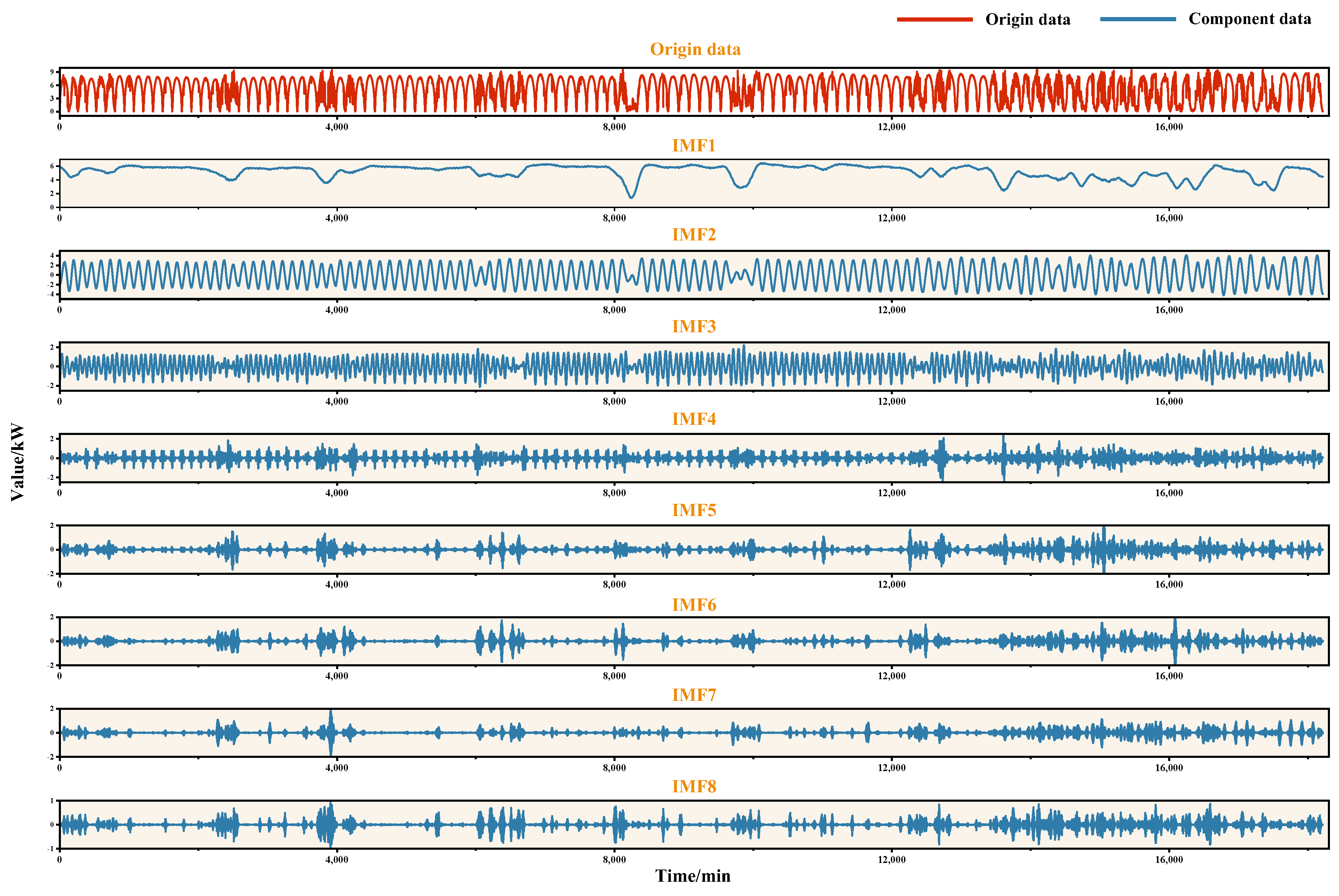
With the aim of assessing the complexity inherent in time series more precisely, the VMD algorithm serves to decompose the historical power sequence related to photovoltaic power generation into eight sub-questions, as shown in Figure 4. Then, the sample entropy of all modal components along with the original photovoltaic power sequence are computed. Sample entropy results for each component are shown in Table 2. In Table 2, the entropy values of IMF1 to IMF8 are 0.028, 0.062, 0.124, 0.151, 0.186, 0.266, 0.324, and 0.360, respectively. The sample entropy of the original sequence equals 0.202. The entropy values for IMF6, IMF7, and IMF8 exceed those of the original sequence, which indicates that their complexity is very high. Therefore, IMF6, IMF7, and IMF8 are merged into a single reconstructed component HSE-IMF by using add operation. The entropy values of IMF3, IMF4, and IMF5 are less than the original sequences, but greater than 0.10. Thus, they are regarded as medium entropy values sequences. The entropy values of IMF1 and IMF2 are less than 0.1, which are classified as low entropy value sequences. The reorganization results of all modal components are shown in Table 3.

4.5. Validation of Prediction Results Based on IRIME Algorithm

For the purpose of verifying the predictive capability of this paper’s proposed algorithm, using GRU, BIGRU, VMD-BIGRU, VMD-SE-BIGRU, VMD-SE-RIME-BIGRU, and the model proposed in this paper to predict the PV output power. The comparison of model prediction results is shown in Table 4. The comparison chart of prediction results curves using different methods of various types is shown in Figure 5.
It can be clearly seen from Table 4 that in the prediction results for sunny days, compared with the EMD-BIGRU and EEMD-BIGRU models, the MAE of the proposed model decreased by 24.10% and 16.07%, respectively; the MAPE decreased by 4.56% and 2.42%, respectively; the RMSE decreased by 11.35% and 0.36%, respectively; and the R2 value increased by 14.05‰ and 3.72‰, respectively. It can thus be concluded that after the time series data are decomposed by VMD, the prediction error is significantly reduced.
By comparing the VMD-SE-BIGRU model with the VMD-BIGRU model, under three weather conditions (sunny, rainy, and cloudy days), the MAE of the VMD-SE-BIGRU model decreased by 10.84%, 12.04%, and 15.45%, respectively; the MAPE decreased by 4.96%, 8.01%, and 5.60%, respectively; the RMSE decreased by 12.32%, 0.77%, and 14.13%, respectively; and the R2 value increased by 0.50‰, 0.81‰, and 0.51%, respectively. It can be observed that applying sample entropy to reconstruct the decomposed time series can significantly improve the accuracy and stability of predictions.
When the proposed method is compared with the above-mentioned seven prediction models, the VMD-SE-IRIME-BIGRU model achieves the highest prediction accuracy, whether in stable sunny conditions or in rainy and cloudy conditions where photovoltaic power fluctuates significantly. Compared with the VMD-SE-RIME-BIGRU model, the MAE of the VMD-SE-IRIME-BIGRU model decreased by 28.59%, 35.79%, and 21.95%, respectively; the MAPE decreased by 3.07%, 3.03%, and 6.48%, respectively; and the RMSE decreased by 23.47%, 12.33%, and 23.49%, respectively. The research results show that the IRIME algorithm exhibits stronger optimization performance, thereby enabling the VMD-SE-IRIME-BIGRU model to improve the accuracy and reliability of photovoltaic power generation prediction.
From Figure 5, it is observed that the prediction outcomes of the proposed approach show strong agreement with real-world data, with predictive accuracy notably exceeding that of other models.
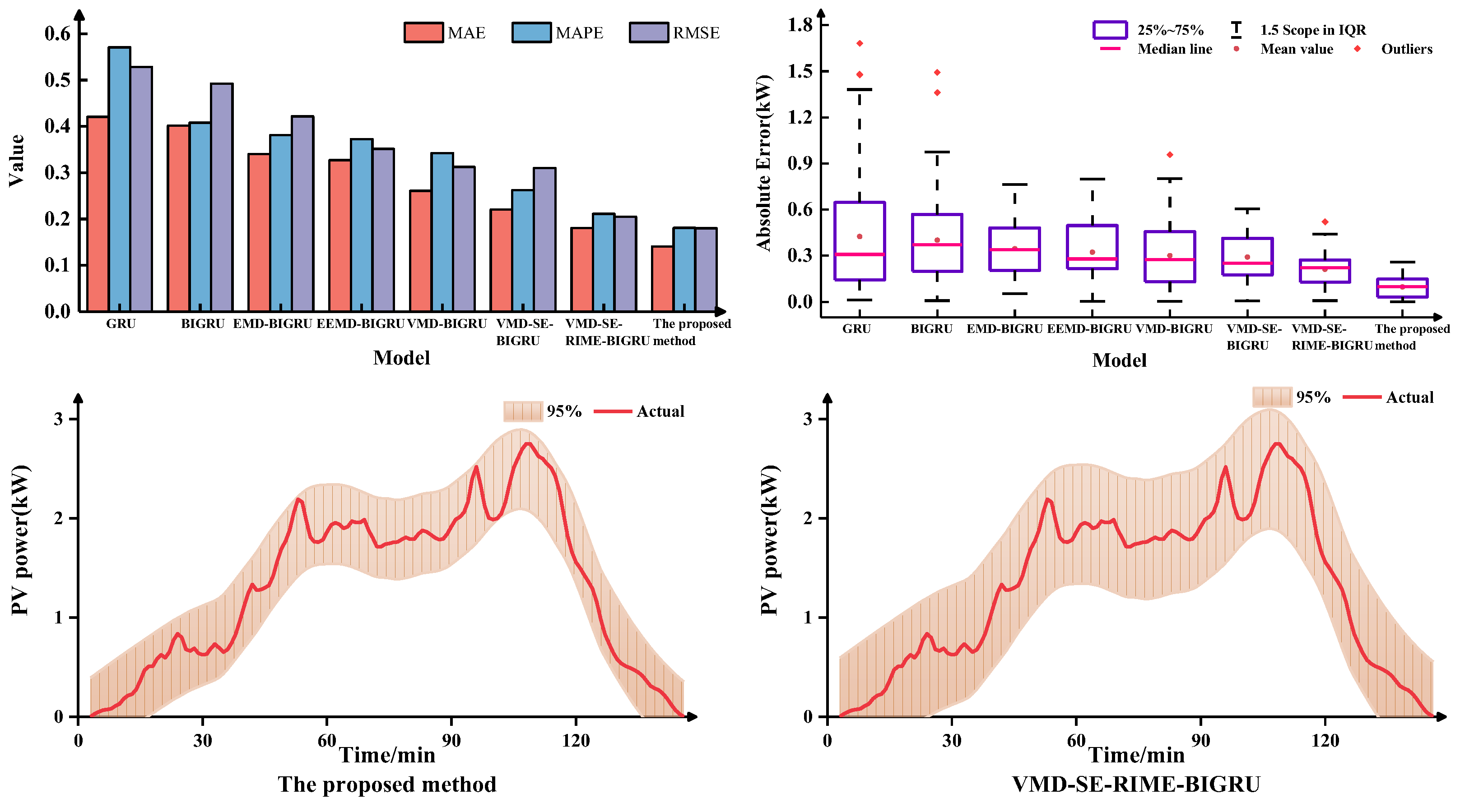
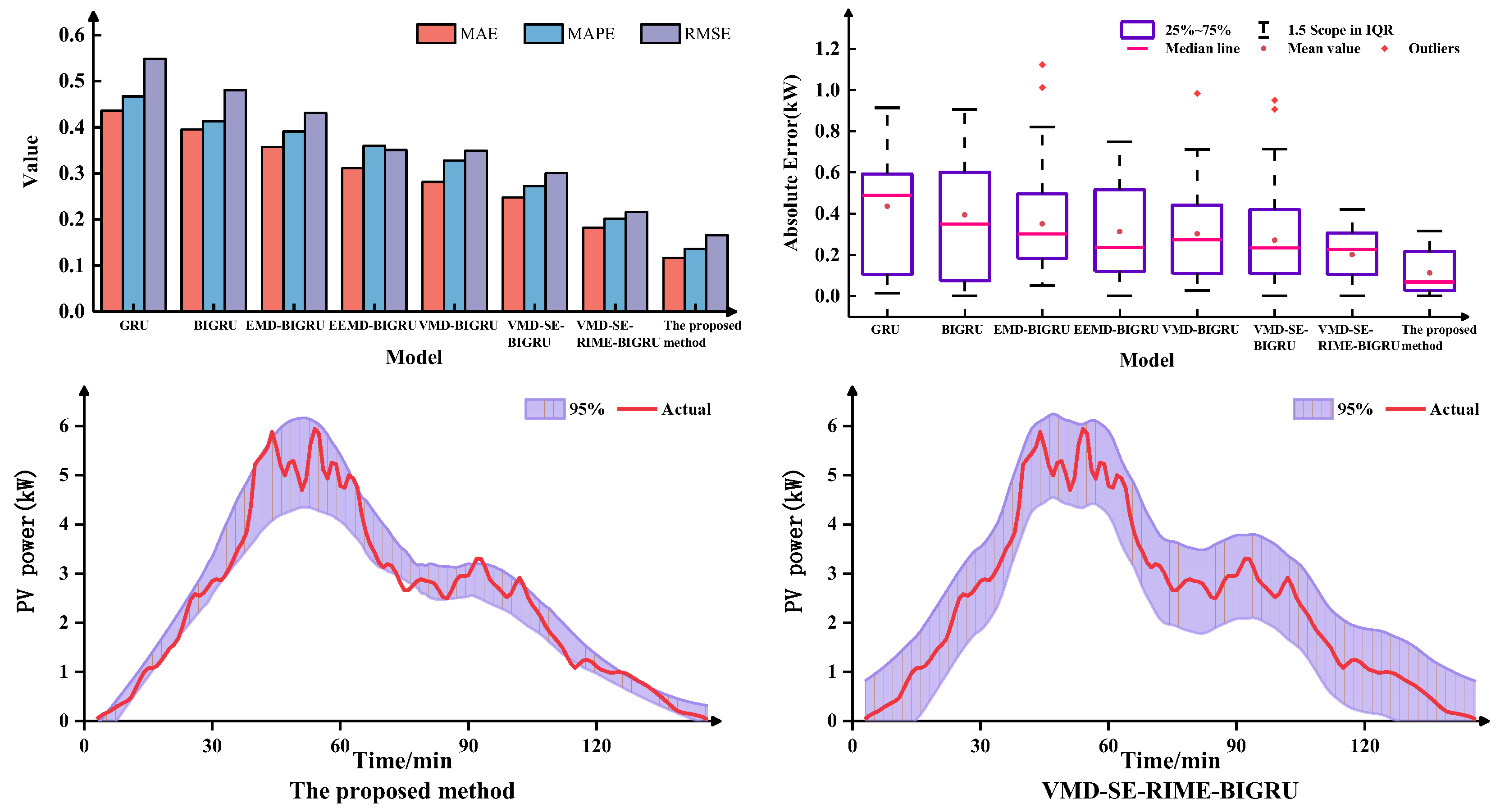
The multinomial indicator error plots, boxplots, and 95% confidence interval of the prediction results of each model are shown in Figure 6, Figure 7, and Figure 8, respectively. As can be seen from the figure, the MAE, MAPE, and RMSE of the proposed method are lowest under different weather characteristics, which indicates that the prediction accuracy is the highest. Furthermore, the prediction error absolute average value and median line of the proposed model is significantly smaller than that of other models, and the number of outliers is also less than that of other models. Compared to VMD-SE-RIME-BIGRU, the proposed method also exhibits clearer boundaries within the 95% confidence interval, further validating the effectiveness of the IRIME algorithm.
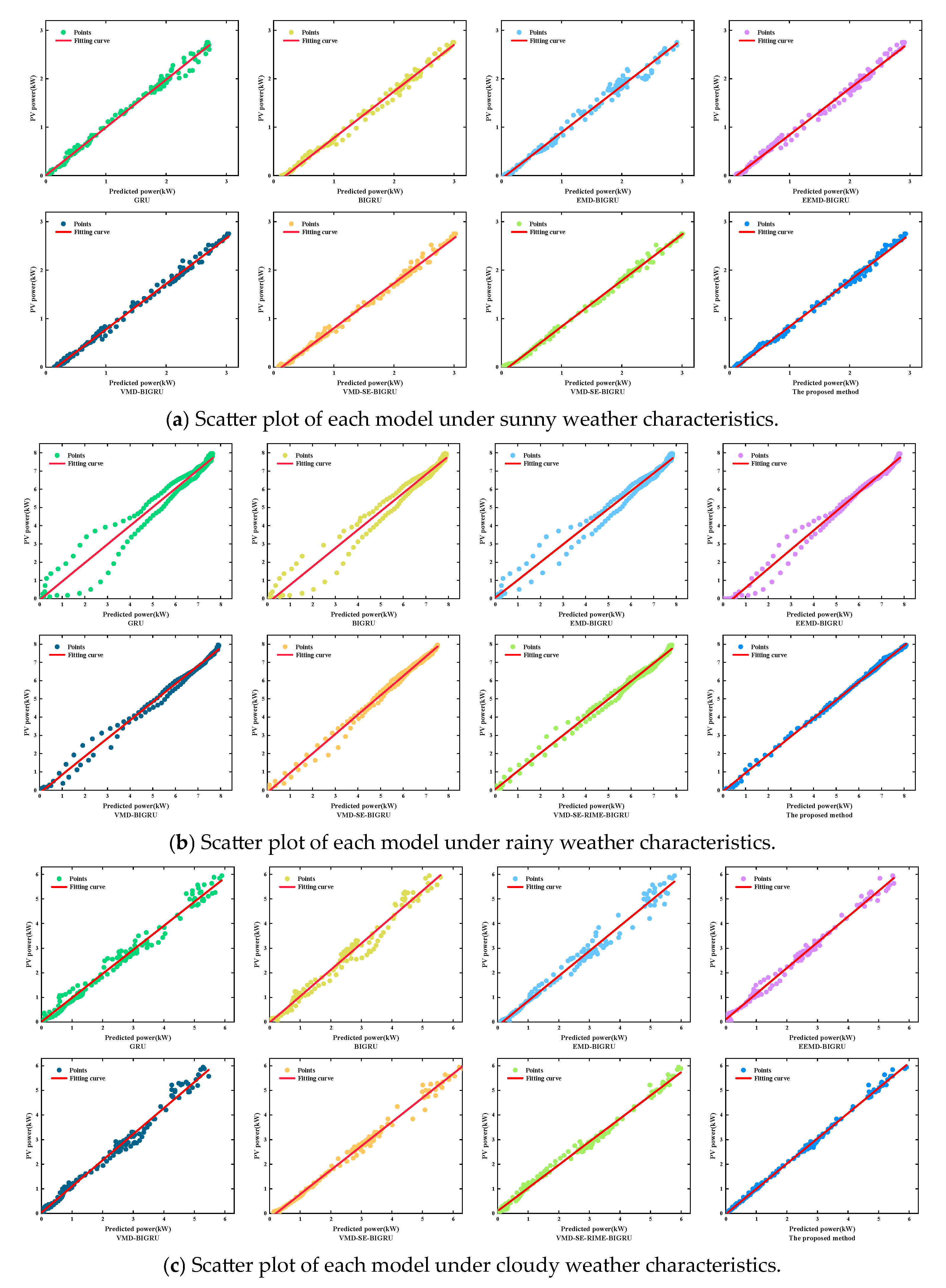
By plotting scatter plots of actual values and predicted values, we can more intuitively demonstrate the overall relationship trends and prediction performance of each model. The R2 value represents the degree of correlation between actual values and predicted values, with a larger value indicating a stronger correlation. As illustrated in Figure 9, the proposed model’s R2 value reaches 0.99, demonstrating that the model possesses the highest prediction accuracy compared to other models.
Figure 10 presents the iterative process of optimal fitness values for RIME and IRIME. As shown in Figure 10, under three typical weather conditions (sunny, rainy, and cloudy days), compared with the RIME algorithm, the iteration speed of the IRIME algorithm increased by approximately 40.63% on average, and the number of iterations decreased by 43.75% on average. In other words, the IRIME algorithm can identify optimal solutions faster. Furthermore, it can be seen from Appendix A that the average running time of the proposed model in this paper is approximately 78 min, and its average single-point prediction time is about 1.41 milliseconds. This can meet the requirement of rapid response for short-term prediction in practical engineering and ensure the feasibility of deployment.

5. Conclusions

To address the issue of low PV prediction accuracy induced by the randomness and uncertainty of PV power generation, this paper proposes a short-term PV power forecasting approach integrating variational modal decomposition and the IRIME optimization algorithm. From the experimental findings, the following conclusions are derived:
  • VMD is capable of decomposing nonlinear and non-smooth time series data into a number of relatively smooth components, which effectively mitigates the impact of modal component mixing.
  • SE is used to reconstruct modal components, yielding components of high, medium, and low frequencies that can reduce the complexity and computation of the time series.
  • Introducing a convergence factor into the RIME algorithm enables enhancement of the algorithm’s global and local search performance, which notably reduces the time needed for complex computations. Relative to the RIME algorithm, IRIME can enhance convergence rate and decrease the number of iterations.
  • By combining the advantages of the VMD, SE, and IRIME algorithms, the hybrid prediction model put forward in this study markedly enhances the predictive accuracy for PV power generation while effectively reducing prediction errors.
Although the model put forward in this article can enhance the stability of raw data and boost prediction accuracy, it also has certain limitations that require consideration in future studies. Future research may explore the introduction of more efficient algorithms or optimization techniques to effectively reduce the model’s computational burden. Secondly, addressing the limitation of the current study—where weather is only classified into three typical types for model training—considering that environmental differences among different PV power plants in practical engineering may lead to more complex weather conditions, subsequent efforts will systematically collect meteorological data from multiple regions to establish a more refined weather classification system. Furthermore, on the basis of expanding multi-dimensional meteorological feature inputs, systematic comparative experiments will be conducted to comprehensively evaluate the performance of the model proposed in this study and advanced time series models under complex operating conditions, thereby further verifying the robustness of the proposed method in a wider range of scenarios.

Author Contributions

Conceptualization, L.X. and L.L.; methodology, L.X. and L.L.; software, X.X.; validation, L.L. and X.X.; formal analysis, J.C.; data curation, H.C. and H.L.; writing—original draft preparation, L.L.; writing—review and editing, L.X. and L.L.; project administration, J.C.; funding acquisition, L.X. and J.C. All authors have read and agreed to the published version of the manuscript.

Funding

This research was funded by Lingling Xie, grant number 2021GXNSFAA220132.

Institutional Review Board Statement

Not applicable.

Informed Consent Statement

Not applicable.

Data Availability Statement

The data that support the findings of this work are available from the corresponding author upon request.

Conflicts of Interest

Authors Jiajia Cai, Hanzhong Cui, and Haoyuan Li were employed by China Resources New Energy (Tengxian) Co., Ltd. All authors declare that the research was conducted in the absence of any commercial or financial relationships that could be construed as a potential conflict of interest.

Appendix A

Table A1. Computation time and single-step prediction time of all model.
Weather TypeModelAverage RuntimeAverage Single-Point Prediction TimeWeather TypeModelAverage RuntimeAverage Single-Point Prediction Time
SunnyGRU8 min 07 s0.23 msRainyGRU9 min 11 s0.14 ms
BIGRU10 min 26 s0.35 msBIGRU11 min 57 s0.29 ms
EMD-BIGRU17 min 42 s1.09 msEMD-BIGRU22 min 53 s1.18 ms
EEMD-BIGRU19 min 43 s1.39 msEEMD-BIGRU23 min 44 s1.42 ms
VMD-BIGRU20 min 04 s1.31 msVMD-BIGRU23 min 17 s1.27 ms
VMD-SE-BIGRU24 min 49 s1.29 msVMD-SE-BIGRU27 min 09 s1.41 ms
VMD-SE-RIME-BIGRU92 min 33 s1.47 msVMD-SE-RIME-BIGRU98 min 54 s1.36 ms
The proposed method77 min 42 s1.43 msThe proposed method80 min 47 s1.39 ms
CloudyGRU8 min 45 s0.21 ms
BIGRU12 min 39 s0.33 ms
EMD-BIGRU19 min 48 s1.26 ms
EEMD-BIGRU23 min 57 s1.29 ms
VMD-BIGRU22 min 41 s1.37 ms
VMD-SE-BIGRU25 min 52 s1.20 ms
VMD-SE-RIME-BIGRU94 min 07 s1.44 ms
The proposed method79 min 12 s1.40 ms

References

  1. Wang, J.; Zhou, Y.; Li, Z. Hour-ahead photovoltaic generation forecasting method based on machine learning and multi objective optimization algorithm. Appl. Energy 2022, 312, 118725. [Google Scholar] [CrossRef]
  2. International Renewable Energy Agency (IRENA). 2025 Renewable Energy Installed Capacity Statistics Report; International Renewable Energy Agency (IRENA): Masdar City, United Arab Emirates, 2025; Available online: https://www.irena.org/ (accessed on 12 June 2025).
  3. Zhang, Y.; Pan, Z.; Wang, H.; Wang, J.; Zhao, Z.; Wang, F. Achieving wind power and photovoltaic power prediction: An intelligent prediction system based on a deep learning approach. Energy 2023, 283, 129005. [Google Scholar] [CrossRef]
  4. Wu, Y.; Chen, Z.; Chen, R.; Chen, X.; Zhao, X.; Yuan, J.; Chen, Y. Stochastic optimization for joint energy-reserve dispatch considering uncertain carbon emission. Renew. Sustain. Energy Rev. 2025, 211, 115297. [Google Scholar] [CrossRef]
  5. Zhang, R.; Bu, S.; Zhou, M.; Li, G.; Zhan, B.; Zhang, Z. Deep reinforcement learning based interpretable photovoltaic power prediction framework. Sustain. Energy Technol. Assess. 2024, 67, 103830. [Google Scholar] [CrossRef]
  6. Wohlschlager, D.; Janis, R.; Iris, S.; Anika, N.-R.; Magnus, F. Green Light for Bidirectional Charging? Unveiling Grid Repercussions and Life Cycle Impacts. Adv. Appl. Energy 2024, 16, 100195. [Google Scholar] [CrossRef]
  7. Ge, J.; Gao, B.; Zhou, Z.; Pang, Z.; Wang, X.; Hong, H.; Zhan, Z. Application of artificial intelligence technology in photovoltaic power generation prediction. J. Phys. Conf. Ser. 2024, 2728, 12036. [Google Scholar] [CrossRef]
  8. Khanali, M.; Ghasemi-Mobtaker, H.; Varmazyar, H.; Mohammadkashi, N.; Chau, K.; Nabavi-Pelesaraei, A. Applying novel eco-exergoenvironmental toxicity index to select the best irrigation system of sunflower production. Energy 2022, 250, 123822. [Google Scholar] [CrossRef]
  9. Girdhani, B.; Agrawal, M. Prediction of daily photovoltaic plant energy output using machine learning. Energy Sources Part A Recovery Util. Environ. Eff. 2024, 46, 5904–5924. [Google Scholar] [CrossRef]
  10. Drałus, G.; Mazur, D.; Kusznier, J.; Drałus, J. Application of Artificial Intelligence Algorithms in Multilayer Perceptron and Elman Networks to Predict Photovoltaic Power Plant Generation. Energies 2023, 16, 6697. [Google Scholar] [CrossRef]
  11. Li, H.; Wu, W.; Chen, W.; Zhang, M. RTI-Net: Physics-informed deep learning for photovoltaic power forecasting. Renew. Energy 2025, 256, 124152. [Google Scholar] [CrossRef]
  12. Guo, X.F.; Zhan, Y.; Zheng, D.; Li, L.Y.; Qi, Q. Research on short-term forecasting method of photovoltaic power generation based on clustering SO-GRU method. Energy Rep. 2023, 9, 786–793. [Google Scholar] [CrossRef]
  13. Roldán-Blay, C.; Abad-Rodríguez, M.F.; Abad-Giner, V.; Serrano-Guerrero, X. Interval-based solar photovoltaic energy predictions: A single-parameter approach with direct radiation focus. Renew. Energy 2024, 230, 120821. [Google Scholar] [CrossRef]
  14. Khan, Z.A.; Hussain, T.; Baik, S.W. Dual stream network with attention mechanism for photovoltaic power forecasting. Appl. Energy 2023, 338, 120916. [Google Scholar] [CrossRef]
  15. Cao, L.; Yang, H.; Zhou, C.; Wang, S.; Shen, Y.; Yuan, B. Photovoltaic Short-Term Output Power Forecast Model Based on Improved Complete Ensemble Empirical Mode Decomposition with Adaptive Noise–Kernel Principal Component Analysis–Long Short-Term Memory. Energies 2024, 17, 6365. [Google Scholar] [CrossRef]
  16. Zhang, H.; Shi, J.; Zhang, C. A hybrid ensembled double-input-fuzzy-modules based precise prediction of PV power generation. Energy Rep. 2022, 8, 1610–1621. [Google Scholar] [CrossRef]
  17. Ma, D.; Xie, R.; Pan, G.; Zuo, Z.; Chu, L.; Ouyang, J. Photovoltaic Power Output Prediction Based on TabNet for Regional Distributed Photovoltaic Stations Group. Energies 2023, 16, 5649. [Google Scholar] [CrossRef]
  18. Kumar, A.; Maan, V.S.; Choudhary, R.; Saini, M. Availability evaluation of solar photovoltaic systems using markov modeling and cuckoo search algorithm. J. Intell. Fuzzy Syst. 2024, 46, 2261–2272. [Google Scholar] [CrossRef]
  19. Wang, Q.; Lin, H. Ultra-short-term PV power prediction using optimal ELM and improved variational mode decomposition. Front. Energy Res. 2023, 11, 1140443. [Google Scholar] [CrossRef]
  20. Hu, Z.; Gao, Y.; Ji, S.; Mae, M.; Imaizumi, T. Improved multistep ahead photovoltaic power prediction model based on LSTM and self-attention with weather forecast data. Appl. Energy 2024, 359, 122709. [Google Scholar] [CrossRef]
  21. Xiang, X.; Li, X.; Zhang, Y.; Hu, J. A short-term forecasting method for photovoltaic power generation based on the TCN-ECANet-GRU hybrid model. Sci. Rep. 2024, 14, 6744. [Google Scholar] [CrossRef]
  22. Ekinci, E. A comparative study of LSTM-ED architectures in forecasting day-ahead solar photovoltaic energy using Weather Data. Computing 2024, 106, 1611–1632. [Google Scholar] [CrossRef]
  23. Zang, H.; Chen, D.H.; Liu, J.X.; Cheng, L.L.; Sun, G.Q.; Wei, Z.N. Improving Ultra-Short-Term Photovoltaic Power Forecasting Using a Novel Sky-Image-Based Framework Considering Spatial-Temporal Feature Interaction. Energy 2024, 293, 130538. [Google Scholar] [CrossRef]
  24. Cheikh, G.; Boudour, A.; Naourez, B.; Kamil, A.; Hadj, A.; Amel, K.; Ala, S. Transformer-Based Deep Neural Networks for Short-Term Solar Power Prediction in the Middle East and North Africa Regions. Eng. Appl. Artif. Intell. 2025, 160, 111848. [Google Scholar] [CrossRef]
  25. Kumar, M.; Namrata, K.; Kumari, N. Hyper-parametric improved machine learning models for solar radiation forecasting. Concurr. Comput. 2022, 34, 7190. [Google Scholar] [CrossRef]
  26. Yadav, H.K.; Pal, Y.; Tripathi, M.M. Short-term PV power forecasting using empirical mode decomposition in integration with back-propagation neural network. J. Inf. Optim. Sci. 2020, 41, 25–37. [Google Scholar] [CrossRef]
  27. Ban, J.; Pan, X.; Gu, M. Electrical Characteristics Estimation of Photovoltaic Modules via Cuckoo Search—Relevant Vector Machine Probabilistic Model. Front. Energy Res. 2021, 9, 610405. [Google Scholar] [CrossRef]
  28. Jia, L.; Yun, S.; Zhao, Z.; Guo, J.; Meng, Y.; Li, X.; Yang, L. Improving short-term forecasting of solar power generation by using an EEMD-BiGRU model: A comparative study based on seven standalone models and six hybrid models. Int. J. Green Energy 2024, 21, 3135–3158. [Google Scholar] [CrossRef]
  29. Kang, Y.Z.; Yao, Y.K.; Dong, R.L.; Jia, Y.S.; Xie, Q.M.; Wang, J.N. Improved complete ensemble empirical mode decomposition with adaptive noise and composite multiscale permutation entropy for denoising blast vibration signal. Heliyon 2024, 10, 37339. [Google Scholar] [CrossRef]
  30. Zhao, S.; Yang, X.; Li, K.; Li, X.; Qi, W.; Huang, X. Photovoltaic output prediction based on VMD disturbance feature extraction and WaveNet. Front. Energy Res. 2024, 12, 1422728. [Google Scholar] [CrossRef]
  31. Boucetta, L.N.; Amrane, Y.; Chouder, A.; Arezki, S.; Kichou, S. Enhanced Forecasting Accuracy of a Grid-Connected Photovoltaic Power Plant: A Novel Approach Using Hybrid Variational Mode Decomposition and a CNN-LSTM Model. Energies 2024, 17, 1781. [Google Scholar] [CrossRef]
  32. Fu, H.; Zhang, J.; Xie, S.; Huang, X. A Novel Improved Variational Mode Decomposition-Temporal Convolutional Network-Gated Recurrent Unit with Multi-Head Attention Mechanism for Enhanced Photovoltaic Power Forecasting. Electronics 2024, 13, 1605. [Google Scholar] [CrossRef]
  33. Huang, Y.; Wang, A.; Jiao, J.; Xie, J.; Chen, H. Short-Term PV Power Forecasting Based on CEEMDAN and Ensemble DeepTCN. IEEE Trans. Instrum. Meas. 2023, 72, 1–12. [Google Scholar] [CrossRef]
  34. Tao, Z.; Zhang, C.; Xiong, J.; Hu, H.; Ji, J.; Peng, T.; Nazir, M.S. Evolutionary gate recurrent unit coupling convolutional neural network and improved manta ray foraging optimization algorithm for performance degradation prediction of PEMFC. Appl. Energy 2023, 336, 120821. [Google Scholar] [CrossRef]
  35. Su, H.; Zhao, D.; Heidari, A.A.; Liu, L.; Zhang, X.; Mafarja, M.; Chen, H. RIME: A physics-based optimization. Neurocomputing 2023, 532, 183–214. [Google Scholar] [CrossRef]
  36. Yang, B.; Wang, J.; Su, S.; Li, Y.; Wu, P.; Yang, Z.; Li, J. Mismatch losses mitigation of PV-TEG hybrid system via improved RIME algorithm: Design and hardware validation. J. Clean. Prod. 2024, 434, 139957. [Google Scholar] [CrossRef]
  37. Yousri, D.; Fathy, A.; Farag, H.E.Z.; El-Saadany, E.F. Optimal dynamic reconfiguration of thermoelectric generator array using RIME optimizer to maximize the generated power. Appl. Therm. Eng. 2024, 238, 122174. [Google Scholar] [CrossRef]
  38. Zhao, Z.; Yun, S.; Jia, L.; Guo, J.; Meng, Y.; He, N.; Yang, L. Hybrid VMD-CNN-GRU-based model for short-term forecasting of wind power considering spatio-temporal features. Eng. Appl. Artif. Intell. 2023, 121, 105982. [Google Scholar] [CrossRef]
  39. Tao, K.; Zhao, J.; Wang, N.; Tao, Y.; Tian, Y. Short-term photovoltaic power forecasting using parameter-optimized variational mode decomposition and attention-based neural network. Energy Sources Part A Recovery Util. Environ. Eff. 2024, 46, 3807–3824. [Google Scholar] [CrossRef]
  40. Yin, W.; Zhu, S.; Xia, H.; Zhang, J. A hybrid model based on complementary ensemble empirical mode decomposition, sample entropy and long short-term memory neural network for the prediction of time series signals in NPPs. Prog. Nucl. Energy 2024, 176, 105390. [Google Scholar] [CrossRef]
  41. Zhang, Y.; Li, C.; Jiang, Y.; Zhao, R.; Yan, K.; Wang, W. A hybrid model combining mode decomposition and deep learning algorithms for detecting TP in urban sewer networks. Appl. Energy 2023, 333, 120600. [Google Scholar] [CrossRef]
  42. Wang, S.; Shi, J.; Yang, W.; Yin, Q. High and low frequency wind power prediction based on Transformer and BiGRU-Attention. Energy 2024, 288, 129753. [Google Scholar] [CrossRef]
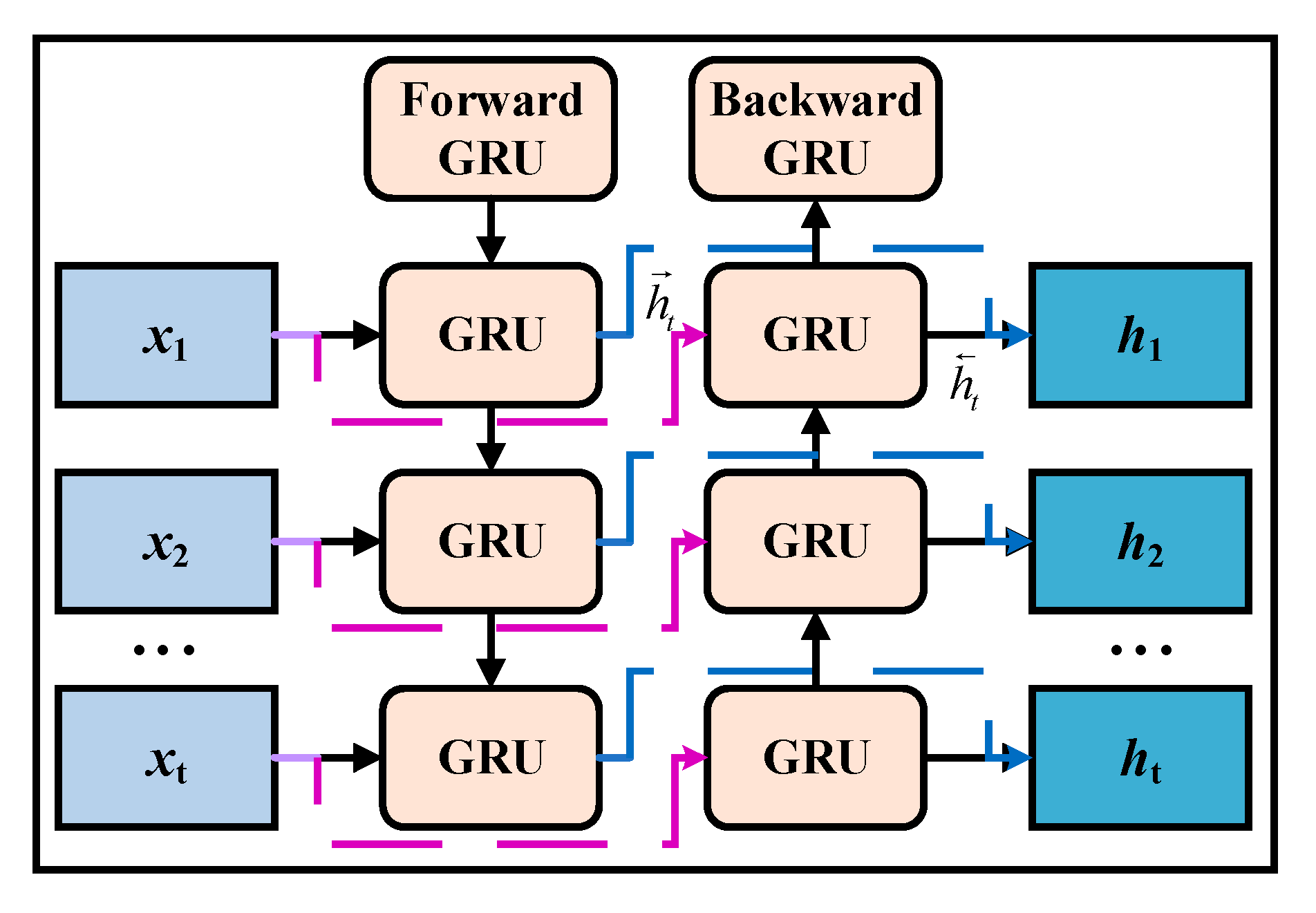
Figure 1. BIGRU network organization.
Electronics 14 03612 g001
Figure 3. Data correlation heat map.
Electronics 14 03612 g003
Figure 4. VMD results for PV power.
Electronics 14 03612 g004
Figure 5. Prediction results of PV power under different weather characteristics. (a) Prediction results of photovoltaic power under sunny conditions; (b) prediction results of photovoltaic power under rainy conditions; (c) prediction results of photovoltaic power under cloudy conditions.
Electronics 14 03612 g005
Figure 6. Results of indicators under sunny weather characteristics.
Electronics 14 03612 g006aElectronics 14 03612 g006b
Figure 7. Results of indicators under rainy weather characteristics.
Electronics 14 03612 g007
Figure 8. Results of indicators under cloudy weather characteristics.
Electronics 14 03612 g008
Figure 9. Scatter plot of each model under different weather characteristics.
Electronics 14 03612 g009
Figure 10. The iteration process of optimal fitness value of RIME and the IRIME.
Electronics 14 03612 g010
Table 2. Sample entropy results for each component.
ComponentSEComponentSE
IMF10.028IMF60.266
IMF20.062IMF70.324
IMF30.124IMF80.360
IMF40.151Original0.202
IMF50.186
Table 3. Reorganization results of all modal components.
ComponentReconstructed Component
HSE-IMFIMF6, IMF7, IMF8
MSE-IMFIMF3, IMF4, IMF5
LSE-IMFIMF1, IMF2
Table 4. Comparison of different model prediction results.
Weather TypeModelEvaluation Metrics
PMAEPMAPEPRMSER2
SunnyGRU0.387242.89%0.48180.9623
BIGRU0.330335.73%0.43240.9786
EMD-BIGRU0.306231.88%0.37170.9821
EEMD-BIGRU0.276929.74%0.33070.9922
VMD-BIGRU0.232427.32%0.32950.9959
VMD-SE-BIGRU0.207222.36%0.28890.9964
VMD-SE-RIME-BIGRU0.159816.09%0.20580.9975
The proposed method0.114113.02%0.15750.9987
RainyGRU0.435946.70%0.54820.9528
BIGRU0.394941.29%0.48020.9617
EMD-BIGRU0.357239.07%0.4310.9739
EEMD-BIGRU0.311236.01%0.35070.9823
VMD-BIGRU0.281532.79%0.34950.9828
VMD-SE-BIGRU0.247627.19%0.30010.9833
VMD-SE-RIME-BIGRU0.181620.10%0.21630.9848
The proposed method0.116613.62%0.16550.9952
CloudyGRU0.420657.08%0.52870.9603
BIGRU0.401840.79%0.49240.9694
EMD-BIGRU0.340638.14%0.42170.9759
EEMD-BIGRU0.327237.27%0.35150.9822
VMD-BIGRU0.260934.24%0.31250.9876
VMD-SE-BIGRU0.220626.23%0.31010.9884
VMD-SE-RIME-BIGRU0.180421.13%0.20520.9893
The proposed method0.140818.10%0.17990.9904
Disclaimer/Publisher’s Note: The statements, opinions and data contained in all publications are solely those of the individual author(s) and contributor(s) and not of MDPI and/or the editor(s). MDPI and/or the editor(s) disclaim responsibility for any injury to people or property resulting from any ideas, methods, instructions or products referred to in the content.