Abstract
As low-voltage distribution networks incorporate increasingly diverse loads, series arc faults exhibit weak characteristics that are easily masked by load currents, leading to high misjudgment rates in traditional detection methods. This paper proposes a series arc fault detection method based on an improved Light Gradient Boosting Machine (LightGBM) model. First, a test platform containing 12 household loads was built to collect arc data from both individual and composite loads. Composite loads refer to composite load conditions where multiple devices are running simultaneously and arcing occurs on some loads. To address the challenge of feature extraction, Variational Mode Decomposition (VMD) is employed to isolate the fundamental frequency component. To enhance high-frequency arc characteristics, singular value decomposition (SVD) is then applied. A multidimensional statistical feature set—comprising peak-to-peak value, kurtosis, and other indicators—is constructed. Finally, the LightGBM algorithm is used to identify arc faults based on these features. To overcome the LightGBM model’s limited ability to focus on hard-to-classify samples, a dynamic weighted hybrid loss function is developed. Experiments demonstrate that the proposed method achieves 98.9% accuracy across 223,615 sample groups. When deployed on STM32H723VGT6 hardware, the average fault alarm time is 83.8 ms, meeting requirements.
1. Introduction
The rapid upgrade of urban and rural power infrastructure, along with the widespread adoption of low-voltage distribution networks, has significantly improved both power supply reliability and the electricity experience for end users [1,2]. However, the growing complexity of distribution network topology, along with the widespread adoption of diverse electrical appliances, has significantly heightened the pressure on system operation and maintenance. Extending equipment maintenance cycles has directly contributed to the increased frequency of line failures [3]. Statistics show that in China, over 100,000 fires occur annually, with more than 80% attributed to arc faults [4]. Among electrical hazards, fire accidents caused by arc discharge deserve particular attention due to their extreme temperatures [5]. Studies have shown that even a small current of 0.5 A can generate an arc temperature between 2000 °C and 3000 °C, high enough to easily ignite most combustible materials [6,7]. Disaster statistics from the National Fire Protection Association (NFPA) show that over 60% of major fires in residential areas are closely linked to arc anomalies [8,9]. In its proposed amendments to the 2026 edition of the National Electrical Code (NEC), the NFPA has further emphasized arc flash protection. Each year, in the United States, 350 to 1050 arc flash incidents occur, causing more than 2000 injuries [10]. Detecting arc faults remains challenging. Although researchers have acknowledged that the resistive nature of series arcs reduces the sensitivity of traditional relay protection devices [11], practical conditions complicate the issue. The dynamic interference of composite loads and the masking effect of the fundamental current create significant obstacles [12]. The problem is particularly acute when the fault current is below 3 A, as its time–frequency characteristics closely overlap with those of normal loads. This overlap often leads to detection failures, making arc fault identification a critical bottleneck for power distribution safety.
Currently, the academic community has developed two main research approaches for arc detection technology: physical feature sensing and electrical signal analysis. The first approach detects arc faults by capturing radiation signals such as sound, light, and heat. However, because arc fault locations are unpredictable, sensor deployment is costly, and the detection range remains limited. In practice, devices such as ultraviolet sensors and arc protectors are mainly installed in switch cabinets to monitor arc flashes [13]. The second approach relies on analyzing voltage signal distortions but is constrained by its dependence on prior fault prediction [14]. Roscoe G. W. et al. [15] employed photodetector outputs and detection circuit breakers as response signals to accurately identify arc faults and reduce misjudgments. Parikh P. et al. [16] applied modern sensor technology to capture photoacoustic pressure signals generated during arc events in wiring rooms, extracting unique features that enable reliable protection, even under low-load currents. Kim C. [17] utilized rod and ring antennas to detect arc electromagnetic radiation in the megahertz band, proposing portable low-amplitude antennas capable of identifying low-voltage arc faults. The different arc stages could be distinguished based on the onset time of the captured signals and their spectral content. Wu Ziran et al. [18] decomposed signals into multi-layer intrinsic IMFs and applied holographic Hilbert transform analysis to generate a high-dimensional amplitude–frequency modulation spectrum with strong discriminative power. Zhang Penghe et al. [19] employed a generalized S-transform with a hyperbolic Gaussian window to extract the time–frequency features of load signals and construct image-based feature samples. Similarly, Cui Ruihua et al. [20] used a signal selection box to intercept experimental data, applied the generalized S-transform, and extracted the RMS value and energy of the 2 kHz component as features, thereby improving arc fault identification accuracy. In contrast, current signals have become a primary research focus due to their universality, with the main technical approaches divided into traditional signal processing and intelligent learning models. In traditional signal processing and analysis, methods such as the Fourier transform and the wavelet transform are commonly used to extract characteristic parameters that can identify AC arc faults by transforming and analyzing current signals in the time, frequency, and time–frequency domains [21,22]. However, this method has certain limitations. On the one hand, when a large number of nonlinear loads are present in the circuit, the harmonics they generate can severely interfere with the current signal, making it challenging for traditional signal processing methods to accurately extract the characteristics of AC arc faults. On the other hand, in complex working conditions, traditional signal processing methods are time-consuming and labor-intensive when setting appropriate thresholds, making it difficult to meet detection requirements across varying conditions.
With the ongoing digital transformation of power systems, data-driven approaches have been increasingly applied across multiple domains. Denis Stanescu et al. [23] proposed a method for characterizing electrical load behavior using phase diagrams, enabling household load identification. More recently, data-driven techniques have also been introduced into AC arc fault detection [24]. For example, intelligent models such as convolutional neural networks (CNNs), long short-term memory networks (LSTMs), and random forests can automatically learn and extract the characteristics of AC arc faults from large datasets of current signal data [25]. Wang Zhaorui et al. proposed a photovoltaic series arc fault detection algorithm based on a lightweight CNN and a feature threshold. They used high-frequency coupling signals as feature signals and combined neural network algorithms with feature threshold methods to detect series arc faults in photovoltaic lines [26]. Huichun Hua et al. [27] proposed a series arc fault detection method using a Newton-optimized sparse kernel support vector machine (NSKsVM) to efficiently identify large-scale arc data. This approach significantly enhanced training speed and classification accuracy, making it well-suited for real-time detection in large datasets. Li Weijun et al. proposed a method for detecting DC series arc faults in photovoltaic grid-connected systems using the random forest algorithm. This method effectively identifies DC series arc faults and is less influenced by external factors, offering good stability [28]. Yu Qiongfang et al. proposed a multi-branch series arc fault detection method using a deep LSTM network [29]. Subsequently, a series arc fault detection method combining a CNN with an LSTM network was proposed, offering a valuable reference for arc fault identification in complex branches [30]. Telford R. D. et al. [31] developed the IntelArc system for arc fault diagnosis. The system integrates time- and frequency-domain feature extraction with a hidden Markov model (HMM) to distinguish normal transient behaviors from arc faults under varying operating conditions. Li J. et al. [32] proposed a feature selection method that combines Euclidean distance, classifier criteria, maximum relevance–minimum redundancy, and clustering indices. Using a random configuration network optimized through variational Bayesian methods, their approach employs the optimal feature set for training and arc fault detection. However, such models still have significant limitations. On the one hand, complex network architectures require substantial hardware resources, making real-time detection challenging in resource-constrained scenarios, such as embedded devices [33]. On the other hand, existing research has not fully addressed arc fault scenarios caused by composite loads in real-world conditions, and the model’s robustness in multi-interference environments remains unverified.
To address the above issues, this paper proposes a series arc fault detection method based on an improved LightGBM model. The key contributions are as follows:
- (1)
- An arc test platform incorporating 12 household appliances was constructed. The analysis showed that arcs in low-current loads exhibited significant waveform distortion, while those in high-current loads displayed a reduced amplitude, extended shoulders, and no waveform distortion. For arcs under compound loads, intermediate-frequency fluctuations were found to be superimposed on the total current. These fluctuations peaked near the zero-crossing points and diminished at the current’s peaks and troughs.
- (2)
- Investigate an extraction method capable of capturing the subtle features of arc faults and enhance the LightGBM model using a loss function to achieve accurate identification of arc faults under both single load and composite load conditions.
- (3)
- An arc fault detection module was designed, and the model was successfully deployed. The experimental results showed that the proposed method detected faults within 100 ms, enabling real-time arc fault detection and demonstrating its practical applicability.
This paper is organized as follows. Section 2 introduces the construction of an arc test platform for data acquisition and analyzes the current characteristics under different operating conditions. Section 3 explores methods for extracting subtle arc fault features. Section 4 introduces an improved LightGBM model with a custom loss function for accurate arc fault identification. Section 5 details the design of the arc fault detection module and the online detection deployment of the proposed model. Finally, Section 6 concludes this paper.
2. Experimental Platform Construction and Data Analysis
2.1. Experimental Platform Construction
Compared to voltage signals, current signals fluctuate more sharply and display stronger high-frequency characteristics during arc events, making them easier to detect. However, directly generating arcs in real household environments poses safety risks. To address this challenge and collect reliable arc fault data under diverse conditions, this paper develops an arc fault detection test platform designed for complex operating scenarios. The platform simulates real power consumption and environmental conditions, as illustrated in Figure 1. The circuit is composed of mains power (220 V/50 Hz), common household loads, and an arc generator, with space reserved at the bus position for installing an arc fault detection device (AFDD). To simulate a real household electricity consumption environment, this paper selected several representative appliances based on the residential load characteristics and energy use patterns identified by Sankhwar et al. [34], including fluorescent lamps (800 W), LED lamps (120 W), bathroom heaters (1000 W), induction cookers (2100 W), microwave ovens (1150 W), kettles (1500 W), refrigerators (600 W), laptops (140 W), vacuum cleaners (1500 W), water dispensers (550 W, heating), air conditioners (1600 W), and washing machines (160 W). Based on their different working principles, loads can be categorized into four types, as shown in Table 1. In addition, following the residential circuit classifications in NFPA 70 [35], all loads were grouped into four branches—lighting, kitchen, bedroom, and bathroom—making the test environment more representative of the actual power demand.
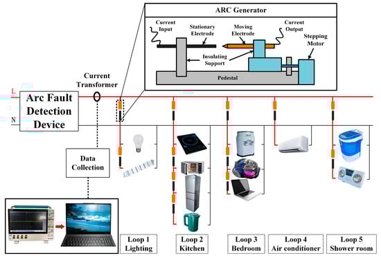
Figure 1.
Schematic diagram of the arc fault test platform.

Table 1.
Load types and rated operating parameters.
The platform’s arc generator uses a stepper motor to move the electrode and produce a continuously burning arc. It simulates air ionization series arcs caused by cable breakage, poor contact at equipment interfaces, and other common faults, serving as a key component of the arc fault detection test platform. During the experiment, the arc generator is connected in series with a load or circuit, and the electrode gap is adjusted to produce a stable and continuous arc, thereby simulating arc faults in various loads. When the arc generator produces an arc, a current transformer and an oscilloscope are used to capture the line current signal, which is then analyzed offline on a PC.
2.2. Data Collection and Analysis
To collect arc data from arcs generated by combined loads (all loads are operated at rated power) in a real environment, this paper presents an arc data acquisition plan (shown in Table 2), which covers the following four experimental conditions: arcing when a single load is operating independently, arcing of a single load in single-circuit operation, arcing of a single load in all-load operation, arcing of multiple loads/multiple circuits in all-load operation.
Table 2.
Arc data acquisition scheme.
The experiment uses a current transformer to collect line current data, which is then converted into a voltage signal through a sampling resistor. The voltage signal across the sampling resistor is captured by an oscilloscope. As shown in Figure 2, the transformer sampling waveforms for both regular operation and arc faults of a single load are displayed. In the figure, the first 60 ms represents the current waveform during regular operation, while the last 60 ms corresponds to the current waveform during an arc fault.
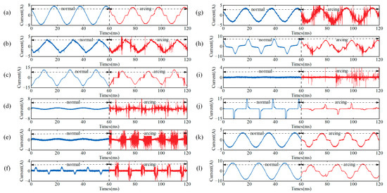
Figure 2.
Signals before and after an arc occurs in a single load. (a) Fluorescent lamp; (b) water dispenser; (c) vacuum cleaner; (d) washing machine; (e) air conditioner; (f) refrigerator; (g) induction cooker; (h) microwave oven; (i) laptop computer; (j) LED lamp; (k) bathroom heater; and (l) kettle.
As shown in Figure 2, when an arc fault occurs in a single load, the changes in the current waveform primarily fall into two categories: The current waveform of the arc in low-current loads (such as fluorescent lamps, refrigerators, and laptops) is significantly distorted, with the arc substantially interfering with the original waveform. The current amplitude of the arc in high-current loads (such as vacuum cleaners, water dispensers, washing machines, air conditioners, induction cookers, and microwave ovens) decreases, and the “shoulder” time is prolonged. However, there is no noticeable distortion in the overall waveform. In both cases, when the load is operating normally, the waveform remains relatively stable, and the similarity between adjacent waveforms is consistent. When an arc fault occurs, the current waveform becomes distorted to varying degrees. The current waveform exhibits a large amount of “high-frequency noise”, primarily concentrated at the zero-crossing point and the peaks and troughs. Characteristics such as variations in the high-frequency components of the signal are observed. The current waveforms of arcs occurring in a single load or multiple loads during the regular operation of all loads are further collected, and the resulting waveforms are shown in Figure 3.
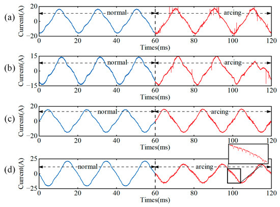
Figure 3.
Signals before and after arcing of a single load or multiple loads when all loads are operating normally. (a) Air conditioner, (b) vacuum cleaner, (c) kitchen circuit, and (d) induction cooker + refrigerator.
As shown in Figure 3, when all loads operate normally, the current waveform remains stable and smooth. However, when arcs occur in some of the loads, certain arc characteristics are masked by the large line current. Therefore, the arc current waveform characteristics, after an arc occurs in a single load, can be classified into three categories: As shown in Figure 3a, loads such as air conditioners generate numerous high-frequency impact signals caused by the inverter, with a signal amplitude exceeding 0.5 V (accounting for 55.6% of the peak-to-peak value of the current signal). These signals are primarily distributed near the peaks, valleys, and zero-crossing point. For motor loads, as shown in Figure 3b, the arc causes random distortion in the current waveform (such as half-wave loss), while the waveforms of other loads remain normal. After the current is superimposed, the waveform amplitude and the high-frequency pulse amplitude decrease (to about 0.15 V, accounting for 18.7% of the peak-to-peak value), resulting in a change in the shape of the current waveform. This change can serve as a key feature in detecting such arc faults. When an arc fault occurs, the load current is relatively small, as shown in Figure 3c. The main current remains largely undistorted; however, the occurrence of high-frequency pulse signals is significantly reduced. The unique phenomenon of a multi-load or multi-circuit arc is illustrated in Figure 3d. When an arc occurs in nonlinear loads, such as induction cookers and refrigerators, the main current is superimposed with an intermediate-frequency fluctuation signal. The signal intensity reaches its peak value when the current crosses zero and then decays at the peak or trough. Its cause is closely related to the interaction between the load’s internal rectifier, inverter, or compressor and the arc. Since these medium-frequency fluctuations are sporadic during regular household load operation, they can serve as a key feature for arc fault detection.
Spectrum analysis of the collected current waveform is performed using a washing machine load as an example, as shown in Figure 4.
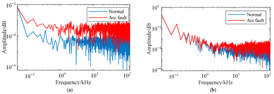
Figure 4.
Spectrum analysis of the arc-free signal and arc fault signal. (a) Arcing in a single load (washing machine). (b) Arcing occurs on a single load (washing machine) while all loads are operating normally.
As shown in Figure 4, when an arc occurs in a single load, the high-frequency component of the arc current increases significantly, with the high-frequency energy across the entire frequency band exceeding that of the normal operating state. However, when all loads are operating and arcing occurs in some loads, the arc signature is masked by the currents of other loads, as the fault load current is smaller than the total mains current. From the perspective of spectrum distribution, under multi-load conditions, the arc energy does not significantly exceed that of the normal state in any specific frequency band. As a result, traditional methods struggle to identify and detect arc faults in such scenarios.
In summary, the diversity of loads will cause significant interference and aliasing to the current signal, resulting in incorrect judgment and missed detection of arc fault methods. In addition, while AI-based methods can offer higher accuracy, edge devices often struggle to meet the high complexity demands of these algorithms, making their implementation in real-world engineering applications challenging. Therefore, there is an urgent need to develop new arc fault detection methods that balance high accuracy with low complexity.
3. Arc Fault Feature Extraction Method Based on VMD-SVD
3.1. Arc Feature Analysis and Extraction Method
While interference and aliasing of current signals between loads complicate arc fault detection, the primary difference between the signals before and after the arc occurs lies in the change in high-frequency components. To extract the high-frequency components from the signal, the low-frequency components must first be removed. To extract the high-frequency components from the signal, the low-frequency components must first be removed completely. Variational Mode Decomposition (VMD) is a technique that decomposes a complex signal into several intrinsic mode functions (IMFs), each corresponding to a distinct frequency component of the signal. Compared to traditional Empirical Mode Decomposition (EMD), VMD offers a more robust theoretical foundation and greater robustness.
The basic idea of VMD is to decompose the signal into several modal functions using variational methods. Each modal function has a limited bandwidth, with spectra that should not overlap as much as possible. The calculation process is as follows:
- The input signal is a discrete signal after pre-emphasis. The goal is to decompose it into intrinsic mode functions , each corresponding to a center frequency . The single-sided spectrum of each modal component is obtained using the Hilbert transform:where is the set of modal functions, is the center frequency of each modal component, is the unit pulse function, is the imaginary unit, and represents the convolution operation.
- Estimate the center frequency of one of the signals and mix it with the analytic signal. This step modulates the modal component signal to the baseband.
- VMD obtains intrinsic mode functions by solving the following variational problem, with each mode function corresponding to a center frequency .where is the partial derivative at sample time n, representing the rate of change of the bandwidth. When the minimum value is reached, the sum of all modal components is guaranteed to equal the input signal.
- By introducing the Lagrange multiplier and the penalty parameter , the constrained optimization problem is transformed into an unconstrained optimization problem:
- Use the Alternating Direction Method of Multipliers (ADMM) to solve the unconstrained optimization problem. ADMM iteratively optimizes and and updates the Lagrange multiplier , gradually approaching the optimal solution.where and represent the Fourier transform and the inverse Fourier transform, respectively. The frequency-domain signal is multiplied by to shift the center frequency of the signal towards zero. is a frequency-domain filter used to control the bandwidth, concentrating the signal near the center frequency. The larger is, the narrower the frequency band becomes.
The adjusted frequency-domain signal is inverse Fourier transformed to obtain the updated modal function. The update of the Lagrange multiplier ensures that the difference between the reconstructed and original signals is gradually reduced. If the following algorithm convergence conditions are met, the modal component signal of VMD is obtained.
Among them, is the preset convergence error.
In this paper, VMD is applied to the current signal to remove the low-frequency component, which is easily masked by other normally operating loads. Only the high-frequency component, which contains a large number of arc characteristics, is retained as the feature for arc detection. Due to the low current of the loads, the high-frequency components are relatively weak when an arc occurs. Therefore, it is essential to develop additional methods to enhance the characteristics of weak arc signals.
3.2. Weak Arc Signal Feature Enhancement Method
In real-world scenarios, the following often occurs: there are many loads in the power consumption environment, and the main circuit current is significant. However, the current in the branch or load where the arc occurs is small, causing the arc fault characteristics of low-power loads to often be covered. If the load power where the arc occurs is significant, the current on the line will be high, and the arc burning will be relatively stable. As a result, the arc characteristics in the current waveform will be weaker. To address the two issues mentioned above, where the arc characteristics in the current waveform collected from the main circuit are not easily detectable, it is necessary to apply feature enhancement techniques to amplify the weak arc characteristics of the load. This paper employs singular value decomposition (SVD) and the reconstruction method to enhance the weak arc characteristics.
Through singular value decomposition and reconstruction, the main features of the signal or large singular values can be effectively preserved, while small singular values or noise are filtered out. Based on the high-frequency signal extracted by VMD (Variational Mode Decomposition), a multidimensional matrix is constructed, as follows: Let the kth IMF (intrinsic mode function) signal obtained from VMD be . Then, the new multidimensional matrix is constructed as:
where . The matrix can be expressed by the following formula:
where is an orthogonal matrix, is a diagonal matrix, and represent the m eigenvalues, i.e., singular values, of the matrix . Expanding Formula (10) yields the following:
Each singular value and its corresponding eigenvector together constitute a feature, and decrease successively. Therefore, when is small, its corresponding eigenvalue will capture more signal features. This paper retains these features when is small and removes the remaining ones to achieve signal noise reduction and feature enhancement.
3.3. Parameter Optimization and Feature Screening
3.3.1. VMD Parameter Optimization
VMD requires setting three key parameters: the penalty factor , the initial center frequency , and the decomposition mode number . In this study, the number of decomposition modes was set to 3, and the penalty parameter α was set to 1000. Specifically, denotes the number of modal components extracted in VMD, while α is the regularization penalty coefficient that balances model complexity and generalization ability. An appropriate combination of parameters ensures that VMD effectively extracts arc features. In contrast, a parameter mismatch can lead to incomplete arc feature extraction, with key features obscured by noise and a significant increase in modal decomposition time. Therefore, it is essential to design the VMD parameters carefully.
This paper removes the fundamental current signal and extracts the high-frequency “burr” characteristic signal through modal decomposition. If the number of decomposed modes (K value) is set too high, it will lead to increased correlation between modes, information redundancy, and the addition of unnecessary modes, resulting in significant feature overlap. When K is too small, extracting the key frequency band of the arc becomes difficult. To avoid the above situation, the modal data are set to 3, and the VMD processing result is shown in Figure 5.
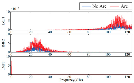
Figure 5.
VMD processing results.
Among the intrinsic mode functions (IMFs) generated by VMD, at least one IMF will contain only the fundamental frequency and low-order harmonic components of the current waveform signal. Such IMFs can be identified through spectrum analysis: if the energy of the fundamental frequency and low-order harmonics is significantly higher than that of the high-order harmonics, they are considered the basic waveform mode and can be filtered out, thereby improving the reconstruction of the modal signal with high-frequency information.
where represents the spectrum of the intrinsic mode , denotes the energy of the fundamental frequency and low-order harmonics, is the fundamental frequency, indicates the energy of the high-frequency signal, and is the threshold for the high-frequency component. Modes that satisfy Formula (8) can be filtered to mitigate the impact of varying loads and current levels on fault detection. The analysis of the three modes reveals that IMF3, with the lowest center frequency, contains the fundamental frequency and low-order harmonics, representing the basic waveform information. IMF1 and IMF2 occupy different frequency bands, with IMF2’s spectrum primarily concentrated in the low-frequency range, blending arc characteristics with standard low-frequency components. The IMF1 spectrum is mainly concentrated in the high-frequency range, reflecting the high-frequency “burr” characteristics of the arc.
3.3.2. SVD Parameter Optimization
The analysis of the waveform characteristics in Section 2.2 indicates that arc occurrences are associated with fewer high-frequency pulses in the current waveform, and these pulses exhibit lower amplitudes. Therefore, weak arc signals must be enhanced to improve detection. Among the three intrinsic mode functions (IMFs) obtained through Variational Mode Decomposition (VMD) of the current signal, IMF3 corresponds to the low-frequency band and reflects the fundamental waveform of the load; so, it does not require enhancement. In contrast, the features of IMF1 and IMF2 need to be amplified to increase the detectability of arc signals.
The effectiveness of SVD signal enhancement depends on the number of retained singular values and their corresponding singular matrices. refers to the number of singular values used to control the degree of data dimensionality reduction. When is set to a high value, noise suppression is insufficient; however, when is set too low, key arc features may be lost. Therefore, this paper uses kurtosis as the evaluation metric and determines the optimal value by analyzing how kurtosis gain varies with different values. The difference in the arc enhancement ratio, with and without enhancement, is calculated by subtracting the kurtosis increase ratio before and after arc signal enhancement. The results are presented in Table 3 and Table 4.
Table 3.
Enhancement signal IMF1 kurtosis value and gain change under different .
Table 4.
Enhancement signal IMF2 kurtosis value and gain change under different .
As shown in Table 3 and Table 4, the difference in kurtosis enhancement ratio between IMF1 and IMF2 initially increases and then decreases as the number of retained singular values changes. When , the difference reaches its peak, indicating that the arc signal characteristics are significantly enhanced through singular value decomposition and reconstruction. This results in the best distinction from non-arc signals. Therefore, this paper determines the optimal number of singular values to be 3.
3.3.3. Statistical Feature Optimization
Arc characteristics can be described by statistical features in both the time and frequency domains. To effectively distinguish arc faults, it is essential to identify electrical parameters that are most sensitive to arc behavior from a wide set of candidates. Common statistical features—including peak-to-peak value, form factor, margin factor, integral coefficient, power spectrum entropy, pulse factor, skewness, kurtosis degree, and integral variance—were evaluated and ranked based on their contribution to arc fault discrimination. The discrimination measure D is defined in Formula (14). Ultimately, six parameters with the highest contributions, such as peak-to-peak value, kurtosis degree, and variance, were selected to form the key pre- and post-arc parameter set.
In the formula, represents the sum of the variance of the data in the kth group that meet the mean interval condition. is the variance of the i-th sample. is the mean of the kth group, which represents the center position of the data in this group. is the sum of the variances of the data within the window, a measure of volatility. is the original data sequence.
Based on this, the key statistical features selected for arc detection are listed in Table 5.
Table 5.
Statistical characteristics of arc detection.
To fully capture arc characteristics, this paper selects feature parameters from both the time and frequency domains. The first four features describe the time-domain waveform and are directly calculated from the current waveform. The last two features are frequency-domain characteristics. The time-domain signal is first converted to the frequency domain, F(n), using the Fast Fourier Transform (FFT), and then, the feature values are calculated according to the formula to form the feature set.
The feature extraction process in this paper is as follows: first, VMD is applied to the collected current signal to obtain three IMF components. The IMF3 component, which represents the load type, is then removed, and the features of IMF1 and IMF2 are enhanced using the SVD feature enhancement method. The statistical features of the enhanced signal are calculated using the formulas in Table 5 to generate a multidimensional feature vector. Figure 6 illustrates the distribution of these selected features under different working conditions.
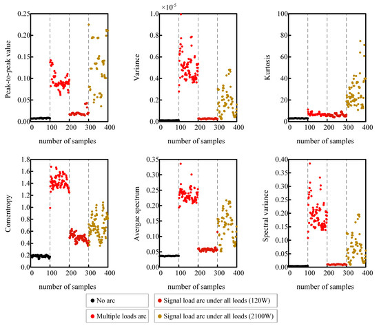
Figure 6.
Distribution of characteristics under different working conditions.
As shown in Figure 6, the calculated values of each feature show no significant changes before and after the arc under different working conditions. Using a fixed threshold for arc detection is prone to both false alarms and missed detections. Therefore, a deep learning model is needed to classify the feature values under different working conditions and enable accurate arc fault detection.
4. Arc Fault Detection Methods
4.1. Improved LightGBM Model
Compared to XGBoost, LightGBM offers several advantages, including faster training speed, lower memory usage, and support for parallel computing. Its algorithm introduces the following optimizations based on the traditional GBDT framework:
- (1)
- Model structure optimization
LightGBM employs a leaf-wise leaf growth strategy and replaces the level-wise layer growth strategy of traditional GBDT through a depth limit mechanism. Compared to the level-wise strategy, which can result in inefficient splitting of low-gain leaves and wasted computational resources, LightGBM’s depth control strategy both maintains growth efficiency and effectively prevents overfitting through hyperparameter tuning.
- (2)
- Training process optimization
LightGBM optimizes the training process and significantly improves model efficiency by employing Gradient-based One-Side Sampling (GOSS), a histogram-based decision tree algorithm, and Exclusive Feature Bundling (EFB). These techniques accelerate training while maintaining accuracy.
LightGBM uses decision trees as weak learners. It iteratively trains multiple weak-performing trees by optimizing residuals, combining them into a strong predictive model. The calculation formula of LightGBM is expressed as follows:
Here, represents the input feature set, denotes the number of decision trees, refers to an individual decision tree, and is the LightGBM prediction value.
The goal of LightGBM model training is to minimize the loss between the predicted result and the actual result , which can be expressed as:
To achieve faster convergence, the negative gradient of the loss function—its first-order derivative—is used in each iteration to approximate the loss function, which can be expressed as:
Traditional LightGBM uses several loss functions, including Binary Cross-Entropy (BCE) Loss and Focal Loss. Each of these loss functions is introduced below.
Binary Cross-Entropy Loss (BCE Loss) is one of the most commonly used loss functions for binary classification tasks. It is defined as follows:
where is the predicted probability value, and is processed by the Sigmoid function and ranges from [0, 1].
It effectively quantifies the deviation between the model’s predicted value and the true label. Since the Sigmoid function restricts the model output to the range [0, 1], BCE Loss can directly process these prediction values, avoiding numerical overflow. Consequently, it is widely used in binary classification tasks. However, BCE Loss has the following limitations:
Sample weight equalization: BCE Loss sums the cross-entropy of all training samples equally, assigning the same weight to each sample.
Imbalanced sensitivity between easy and difficult samples: When a dataset contains both easy-to-classify samples (correctly classified with high confidence) and difficult samples (with ambiguous boundaries), the loss gradient from easy samples disproportionately influences model updates. As a result, the model overemphasizes easy samples during training, leading to poorer classification performance on difficult samples.
Focal Loss addresses class imbalance by dynamically adjusting sample weights during training. Its formula is defined as follows:
Here, represents the similarity between the model’s predicted value and the true label ; the larger is, the closer the prediction is to the label , indicating higher classification accuracy. The parameter is an adjustable focusing factor.
During training, the parameter can be adjusted to modify the model’s focus on difficult-to-classify samples. The term , known as the modulating factor, reduces the weight of easy-to-classify samples, enabling the model to concentrate more on harder cases.
Focal Loss addresses class imbalance by dynamically distinguishing between hard and easy samples. Its core principles are as follows:
The modulating factor reduces the loss contribution of easy-to-classify samples while increasing that of hard-to-classify samples, guiding the model to focus on optimizing performance for difficult cases during training.
Suppression of easy samples: When approaches 1, the sample is considered easy to classify. In this case, the modulating factor approaches 0, reducing its contribution to the loss and effectively lowering the impact of easy samples during training.
Emphasis on hard samples: When is very small, the predicted value deviates significantly from the true label, indicating a misclassified sample. In this case, the modulating factor approaches 1, allowing the loss to remain large and contribute more significantly to model training.
Figure 7 illustrates the output of the loss function for different values of . By comparing Focal Loss and BCE Loss across different values, it is observed that when the predicted probability approaches 0, the loss value of BCE Loss remains relatively small. Due to its symmetric nature, the function assigns equal loss weight to both easy- and hard-to-classify samples, making it difficult for the model to effectively differentiate sample difficulty. In contrast, Focal Loss enhances the model’s focus on hard samples by adjusting the parameter , which increases the loss weight for samples with predicted probabilities close to 0.

Figure 7.
Comparison of Focal Loss and BCE Loss with different .
.
Therefore, this paper proposes a hybrid loss function with dynamic weight adjustment as the optimization objective for model training. The dynamic weight adjustment strategy employs three decay functions—linear decay (LD), cosine decay (CD), and exponential decay (ED)—to adaptively adjust the weighting between the two loss functions at different stages of training. The corresponding decay curves are shown in Figure 8.
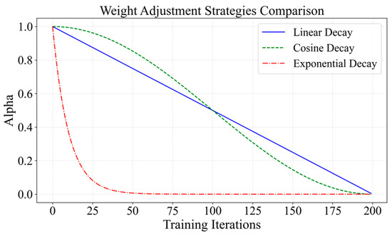
Figure 8.
Comparison of weights of different loss functions as the number of iterations changes.
Figure 8 illustrates that the weight under the linear decay (LD) function decreases linearly as the number of iterations increases. Its advantage lies in enabling a smooth transition from BCE Loss to Focal Loss. During the first half of training (the initial 50% of iterations), the weight of the cosine decay (CD) function remains above 0.5, indicating that BCE Loss primarily optimizes easy-to-classify samples early on. In the later stages, Focal Loss gradually takes precedence to enhance the learning of difficult-to-classify samples. The ED function utilizes exponential weight decay to significantly reduce the weight of BCE Loss in the early stages of training (the first 1/8 stage) and reduces its weight to near zero in the first 1/4 stage. Focal Loss dominates the later training stages. Considering LightGBM’s training characteristics and practical requirements, this paper aims for the model to quickly learn from easy-to-classify samples early on to ensure a low false alarm rate while improving recognition accuracy on difficult-to-classify samples through Focal Loss in the later stages. Because the ED function effectively meets this dynamic requirement, it is chosen as the final strategy for dynamic weight adjustment. The ED model loss function is shown in Figure 9.
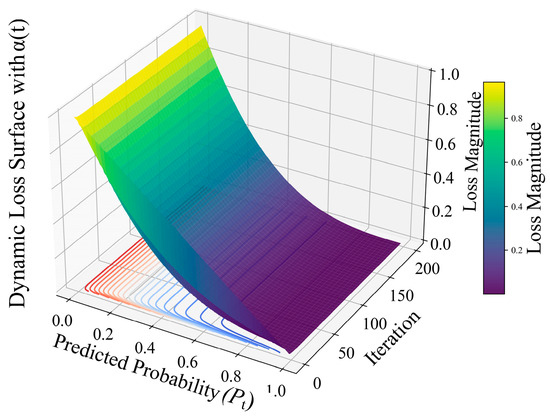
Figure 9.
Trend of the ED model loss function with iteration times and recognition accuracy.
In Figure 9, darker blue indicates lower loss values, while darker red indicates higher loss values. After adopting the ED function, the model’s loss trend over iterations and its recognition accuracy are shown in Figure 9. In the early training stage, BCE Loss dominates, enabling the model to perform balanced optimization across all samples and achieve stable convergence. In the later stages of training, Focal Loss amplifies the penalty for misclassified or uncertain samples, encouraging the model to focus on learning complex cases with ambiguous boundaries. By adjusting the dynamic weight , the model transitions from global optimization to focusing on difficult-to-classify samples. During this process, samples with predicted probabilities near the decision boundary extremes (positive class p → 0 or negative class p → 1) produce larger loss gradients. Consequently, their weight updates during backpropagation are intensified, prompting the model to prioritize correcting high-confidence misclassifications.
4.2. Arc Fault Detection Model Based on Improved LightGBM
Figure 10 illustrates the online arc fault detection process based on the improved LightGBM model.
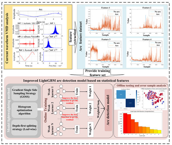
Figure 10.
Improved LightGBM model structure diagram.
First, data from multiple operating conditions are collected according to the experimental plan, and the time series are segmented using a fixed-step moving window. The window length is set to 5000 sampling points, corresponding to one 20 ms period of the AC power frequency, with a step size of 1000 points. Next, VMD is performed on each data window to obtain two sets of intrinsic mode functions (IMFs). The SVD algorithm is then used to enhance the characteristics of each IMF component and extract statistical features in both the time and frequency domains to construct a training dataset. The final dataset consists of 223,615 samples in total, including 85,605 from standard operating conditions and 138,010 from arc fault conditions.
During the development of the LightGBM model, we first separated the high-gradient sample set M and the low-gradient sample set m using the histogram and GOSS algorithms. We then amplified the low-gradient samples by the ratio (1 − M)/m and combined them with the high-gradient samples to train the learner. Second, double optimization is applied to the loss function by using a hybrid loss with dynamically adjusted weights to perform hyperparameter tuning. Among the hyperparameters of the LightGBM model, the maximum depth refers to the number of nodes on the longest path from the root node to a leaf node, which directly affects the complexity of the model. The learning rate controls the update step size, while the update rate controls the actual update amplitude of the model parameters in each iteration. In this study, the maximum depth was set to 31 to prevent overfitting, the learning rate was 0.02, and the update rate was 0.1.
4.3. Experimental Results and Analysis
The constructed dataset is split into a training set and a test set at a 9:1 ratio. The LightGBM model is configured using the optimized hyperparameters, and different loss functions are employed for comparative training. BCE Loss is simple and efficient but often suffers from underfitting. Focal Loss mitigates class imbalance, although it relies on careful parameter tuning. By contrast, the proposed DWM Loss requires slightly longer training time but dynamically adjusts weights according to sample difficulty, offering stronger generalization. The computational time and complexity of the three methods are summarized in Table 6. The model training process is illustrated in Figure 11a,b, which show the curves of model accuracy and loss value, respectively, over the course of network iterations.
Table 6.
Comparison of the different loss functions.
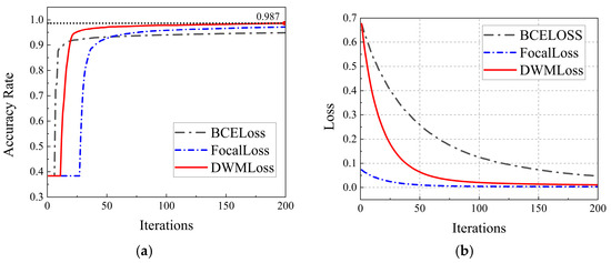
Figure 11.
Comparison of the model training process under different loss functions. (a) Accuracy change curve during training of different loss function models. (b) Loss change curve during training of different loss function models.
As shown in Figure 11a, the LightGBM model experiences short-term underfitting at the start of training. When using BCE Loss, the model tends to prioritize optimizing easy-to-classify samples. However, its limited capacity to handle difficult samples leads to rapid convergence but ultimately results in lower accuracy. The model using Focal Loss shows low learning efficiency on easy-to-classify samples early in training, resulting in slow convergence and limited accuracy improvement. In contrast, the model trained with the dynamic weighted hybrid loss function proposed in this paper has an initial convergence speed between BCE Loss and Focal Loss, but its accuracy improves faster over time, ultimately achieving higher accuracy than the other two models.
As shown in Figure 11b, the loss value changes throughout model training are illustrated. In the initial stage, the weights are fully assigned to easy-to-classify samples, resulting in equal loss values for both the DWM Loss and BCE Loss. As the weights gradually shift toward more complex samples, the loss curves of DWM Loss and Focal Loss begin to align, indicating that both models have reached convergence.
To evaluate the classification performance of the improved LightGBM algorithm for arc fault detection, this study used a test set of 22,362 samples and generated the corresponding confusion matrix. The test set includes two working conditions: with arc and without arc. The confusion matrix for the improved algorithm is visualized in Figure 12. The model testing results are shown in Table 7.
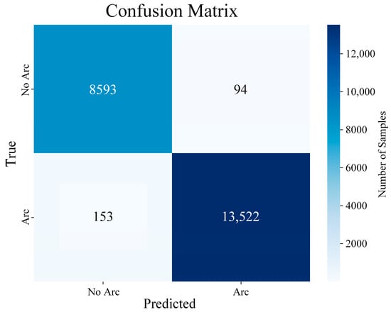
Figure 12.
Confusion matrix of the improved LightGBM arc detection algorithm.
Table 7.
LightGBM identification of arc fault results.
In Table 7, TP stands for true positive; FP stands for false positive; FN stands for false negative; and TN stands for true negative. In the test results, 94 normal operation samples were misjudged as arc faults, and 153 arc fault samples were misidentified as normal. The calculated true positive rate, false positive rate, false negative rate, and true negative rate were 99.3%, 1.8%, 0.7%, and 98.2%, respectively, and the overall accuracy rate was 98.9%. After SVD and VMD extraction, the arc features are obvious, the model training is accurate and relatively stable, and the classification accuracy fluctuates only by ±0.02%. The proposed model was compared with the Arcnet [36] model using a statistical significance test (two-tailed two-proportion Z-test, α = 0.05). The calculated Z-value is 2.674, and the p-value is 0.0075, which shows that the proposed method is more sensitive to arc faults than the Arcnet model, but Arcnet performs better in resisting false detection. Subsequently, the method in this paper effectively reduces the false detection rate in practical applications by adopting a multi-cycle joint decision mechanism. These results demonstrate that the algorithm-optimized LightGBM performs exceptionally well in AC system series arc detection. Its very low false alarm rate indicates that the model effectively avoids overfitting.
To assess the impact of SVD on arc fault detection performance, a comparative experiment was conducted, with the results shown in Table 8. The experimental group processed with SVD exhibited greater distinguishability of arc signals in the feature space, fully validating the effectiveness of the feature enhancement method.
Table 8.
Comparison of model accuracy before and after adding SVD.
5. Hardware Validation of Arc Detection Algorithms
To evaluate the performance of the improved LightGBM arc detection algorithm, this study developed an arc fault detection module, as illustrated in Figure 13. The module features the STM32H723VGT6 microcontroller (STMicroelectronics, Geneva, Switzerland) as its central processor. To meet the flash memory constraints of the MCU, the neural network was first compressed in CUBEMX at a ratio of 8. The trained model was then converted into C code for embedded deployment using the X-Cube-AI expansion package (STMicroelectronics, Geneva, Switzerland) in CUBEMX. After conversion and compression, the model occupied 103.2 KB of ROM and 36.4 KB of RAM, well within the capacity of the STM32H723VGT6. This chip is based on the ARM Cortex-M7 core and includes a 16-bit analog-to-digital converter. It supports a maximum clock frequency of 550 MHz and a sampling rate of up to 3.6 Msps, meeting the data processing and sampling requirements of the algorithm. Additionally, its 1 MB Flash memory and 564 KB RAM provide sufficient resources for deploying the model and executing the algorithm.
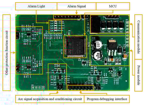
Figure 13.
Arc fault detection device prototype.
To address the issue of model accuracy falling short of ideal values, this paper implements a multi-cycle joint judgment mechanism within the embedded device software algorithm to reduce the risk of false detection. Based on a 98.9% confidence level, a cumulative threshold judgment is applied to the output results. An arc fault alarm is triggered when the cumulative judgment value exceeds the preset threshold over multiple consecutive cycles. The detection process is shown in Figure 14. The average alarm time for each fault condition is 83.8 ms, and all alarm times are within 100 ms, meeting the IEC 62606 standard [37] requirements. The detailed alarm times are presented in Table 9, demonstrating that the system meets the requirements for real-time arc fault detection.
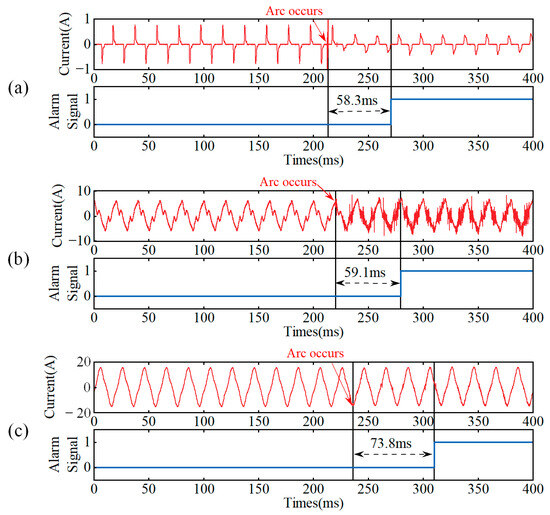
Figure 14.
Arc identification process after hardware deployment. (a) LED arcing. (b) Arc fault in the kitchen circuit. (c) Arc fault in the kitchen + bedroom circuit with full load operation.
Table 9.
Average time of arc fault alarm detection under various working conditions.
To verify the applicability of this model to non-domestic or industrial electrical loads, arc fault detection experiments under two typical loads, namely, an electric drill and an air compressor, were added. The results are shown in Figure 15.
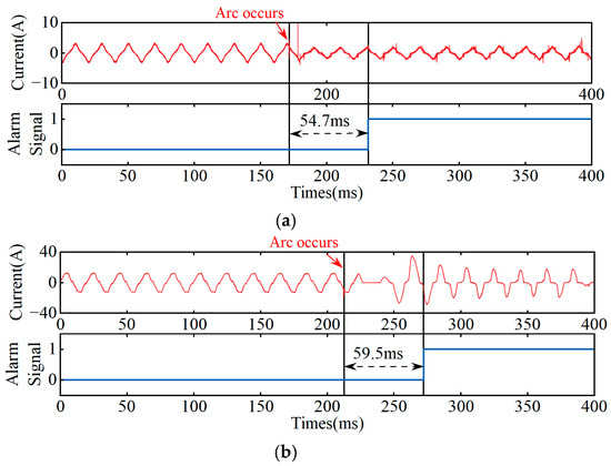
Figure 15.
Arc fault test results. (a) Electric drill. (b) Air compressor.
To further evaluate the effectiveness of the proposed method, several mainstream low-voltage arc detection approaches are selected for comparison. The ArcNet model operates without the need for high sampling rates or data preprocessing, relying solely on CNNs for feature extraction. However, due to its large size, single-sample testing takes slightly longer, and its overall detection speed is slower compared to the method proposed in this paper. Jia Jinwei et al. [38] employed the particle swarm optimization (PSO) algorithm to optimize the weights of the self-organizing map (SOM) network, resulting in a significant improvement in detection accuracy compared to the traditional SOM network. Kou Haowen et al. [39] used short-time Fourier transforms to consider current signals’ time- and frequency-domain characteristics simultaneously. The analysis results were converted into RGB images as network input, enabling high-accuracy arc fault detection. However, the method was limited in the types of loads it could be applied to and did not address composite load testing or edge deployment. The method proposed in this paper is based on household electricity consumption and considers 12 common household electrical loads as well as composite loads. It addresses the challenge of feature extraction in low-voltage distribution networks, where arc fault characteristics are weak and easily obscured. Additionally, the method supports edge deployment of the algorithm and achieves a fault alarm response time of less than 100 ms. Detailed comparison data are presented in Table 10.
Table 10.
Comparison of this method with common algorithms.
6. Conclusions
This paper presents a series arc fault detection method based on an improved LightGBM model, designed to address the challenge of weak arc characteristics in low-voltage distribution networks, which are often masked by other load currents. The main findings are as follows. An arc test platform with 12 household loads was constructed, and current data under various operating conditions were collected and analyzed. For low-current loads, arcs showed pronounced waveform distortion, while high-current loads produced reduced arc amplitude, extended flat shoulders, and no distortion. In composite load scenarios, the total current exhibited intermediate-frequency fluctuations, which peaked near the zero-crossing point and diminished at the waveform’s peaks and troughs. To capture these subtle arc features, a feature extraction method combining VMD and SVD was developed to build an enhanced high-frequency feature set. A dynamic weighted hybrid loss function was further introduced, enabling the improved LightGBM model to achieve 98.9% accuracy on a dataset of 223,615 samples collected from the self-built platform. In addition, an arc fault detection module was designed and deployed, achieving an average alarm response time of 83.8 ms. Overall, the proposed method enables real-time arc fault detection and demonstrates strong practical value for enhancing power distribution safety.
Although the model achieved high accuracy on experimental data, its decision-making process remains difficult to interpret, and its generalization ability requires further enhancement. Future research should therefore incorporate interpretability analysis and broaden application scenarios to strengthen the model’s robustness and adaptability.
Author Contributions
Conceptualization, R.S. and P.Z.; methodology, Y.X.; software, Z.W.; validation, J.W., Y.X. and P.Z.; formal analysis, Y.X.; investigation, J.W.; resources, R.S.; data curation, J.W.; writing—original draft preparation, R.S.; writing—review and editing, R.S.; visualization, Y.X.; supervision, J.W.; project administration, Z.W.; funding acquisition, R.S. All authors have read and agreed to the published version of the manuscript.
Funding
This work was supported by the State Grid Technology Project of the Research and Application of Key Technologies for Measurement and Diagnosis of Low-Voltage Arc Fault with time–space factors from multiple power source loads (Project No. 5700-202455276A-1-1-ZN).
Data Availability Statement
The data presented in this study are available upon request from the corresponding author due to privacy reasons.
Conflicts of Interest
Authors Runan Song, Penghe Zhang, Yang Xue, Zhongqiang Wu and Jiaying Wang were employed by the company China Electric Power Research Institute. The remaining authors declare that the research was conducted in the absence of any commercial or financial relationships that could be construed as a potential conflict of interest.
References
- Yu, K. Research on the Design and Application of High and Low Voltage Distribution Systems in Residential Areas under the Digital Background. Electr. Eng. 2024, 19, 70–72+76. [Google Scholar] [CrossRef]
- Li, A.; Le, C.; Bei, B.; Xiong, J.; Shi, X. A Preliminary Discussion on the Planning of Urban Medium and Low Voltage Distribution Networks. Sci. Technol. Wind. 2021, 188–189. [Google Scholar] [CrossRef]
- Agency, I.E. Growth in Global Electricity Demand Is Set to Accelerate in the Coming Years as Power-Hungry Sectors Expand [EB/OL]. 14 February 2025. Available online: https://www.iea.org/news/growth-in-global-electricity-demand-is-set-to-accelerate-in-the-coming-years-as-power-hungry-sectors-expand (accessed on 19 February 2025).
- Editorial Committee of China Fire and Rescue Yearbook; China Fire Yearbook; Emergency Management Press: Beijing, China, 2022.
- CCTV News. 908,000 Fire Reports Received Throughout the Year. Fire Departments Review Five Characteristics of Fires Across the Country in 2024 [EB/OL]. 24 January 2025. Available online: https://www.119.gov.cn/qmxfxw/mtbd/wzbd/2025/48022.shtml (accessed on 19 February 2025).
- Wang, J. Low Voltage AC Series Arc Fault Detection Based on Multi-Information Fusion. Master’s Thesis, Shandong University of Technology, Zibo, China, 2024. [Google Scholar]
- Underwriters Laboratories Inc. UL Standard for Safety Arc-Fault Circuit-Interrupters, 2nd ed.; Underwriters Laboratories Inc.: New York, NY, USA, 2011. [Google Scholar]
- Association, N.F.P. Home Fires Caused by Electrical Failure or Malfunction [EB/OL]. 14 September 2021. Available online: https://content.nfpa.org/-/media/Project/Storefront/Catalog/Files/Research/NFPA-Research/Electrical/osHomeFiresCausedbyElectricalFailureMalfunction.pdf? (accessed on 19 February 2025).
- Sun, S.; Geng, X.; Fu, G. Research on direct causes of building electrical fire accidents based on the “2–4” model. J. China Saf. Sci. 2020, 30, 93–99. [Google Scholar] [CrossRef]
- Viara, D.A. How Arc Flash Risk Management Is Evolving; EC & M: Belmont, OH, USA, 2025. [Google Scholar]
- Wu, Z.; Wang, D.; Zhao, H.; Wu, L. Analysis of Resistive Leakage Detection Technology to Control the Frequent occurrence of Electrical Fires. Fire Sci. Technol. 2020, 39, 991–993. [Google Scholar]
- Yu, Q.; Hu, Y.; Yang, Y. Fault arc detection based on wavelet features and deep learning. J. Electron. Meas. Instrum. 2020, 34, 100–108. [Google Scholar]
- Park, C.; Lee, K.; Kim, K.; Lim, H.; Park, Y. Evaluation of Time-Based Arc Flash Detection with Non-contact UV Sensor. J. Electr. Eng. Technol. 2024, 19, 1983–1992. [Google Scholar] [CrossRef]
- Cai, B.; Chen, D.; Wu, R.; Wang, X.; Gao, D.; Chen, W. Online detection and protection device for internal fault arc of switchgear. J. Electr. Technol. 2005, 87–91. [Google Scholar] [CrossRef]
- Roscoe, G.W.; Papallo, T.F., Jr. Arc Flash Detection System, Apparatus and Method. U.S. Patent 7,791,846 B2, 7 September 2010. [Google Scholar]
- Parikh, P.; Allcock, D.; Luna, R.; Vico, J. A novel approach for arc-flash detection and mitigation: At the speed of light and sound. IEEE Trans. Ind. Appl. 2014, 50, 1496–1502. [Google Scholar] [CrossRef]
- Kim, C.J. Electromagnetic Radiation Behavior of Low-Voltage Arcing Fault. IEEE Trans. Power Deliv. 2009, 24, 416–423. [Google Scholar] [CrossRef]
- Wu, Z.; Han, Y.; Chen, C. Research on the Characteristics of AC Series Arc Fault Current Based on Holographic Hilbert Spectrum Analysis. Electr. Energy Effic. Manag. Technol. 2024, 8–16. [Google Scholar] [CrossRef]
- Zhang, P.; Qin, Y.; Song, R.; Chen, G. Time frequency analysis and identification of series fault arcs under generalized S-transform. Power Grid Technol. 2024, 48, 2995–3003. [Google Scholar] [CrossRef]
- Cui, R.; Tong, D.; Li, Z. Detection of aviation series arc fault based on generalized S transform. Proc. CSEE 2021, 41, 8241–8250. [Google Scholar]
- Chen, Z. Research on the Application of “Wu’s Shallow Needle Therapy” to Help Sleep Based on Vibration Signals. Master’s Thesis, Fujian University of Technology, Fuzhou, China, 2023. [Google Scholar]
- Zhao, Q. Research on Low-Voltage Series Arc Fault Detection Technology. Master’s Thesis, Shanghai Institute of Electric Power, Shanghai, China, 2022. [Google Scholar]
- Stanescu, D.; Enache, F.; Popescu, F. Smart Non-Intrusive Appliance Load-Monitoring System Based on Phase Diagram Analysis. Smart Cities 2024, 7, 1936–1949. [Google Scholar] [CrossRef]
- Wu, L. Diagnosis Method of Photovoltaic System Series Fault Arc Under Line Impedance Interference Conditions. Master’s Thesis, Xi’an University of Technology, Xi’an, China, 2023. [Google Scholar]
- Li, D. Research on Low-Voltage AC Arc Fault Detection Method Based on Artificial Neural Network. Master’s Thesis, North China Electric Power University, Beijing, China, 2024. [Google Scholar]
- Wang, Z.; He, J.; Li, Z.; Bao, G. Design of photovoltaic series arc fault detection device based on lightweight CNN and feature threshold. Electr. Appl. Energy Effic. Manag. Technol. 2024, 77–85. [Google Scholar] [CrossRef]
- Hua, H.; Fang, D.; Guo, M. Series Arc Fault Identification Based on a Novel Newton-Optimized Sparse Kernel Support Vector Machine. IEEE Trans. Instrum. Meas. 2025, 74, 1–13. [Google Scholar] [CrossRef]
- Li, W.; Li, T.; Su, J. Detection method of series arc fault on photovoltaic DC side based on random forest. Power Supply Util. 2025, 42, 108–115. [Google Scholar]
- Yu, Q.; Lu, W.; Yang, Y. Detection method of multi-branch series fault arc based on deep long short-term memory network. Comput. Appl. 2021, 41 (Suppl. S1), 321–326. [Google Scholar]
- Yu, Q.; Xu, J.; Yang, Y. Detection of complex branch fault arc based on CNNLSTM model. China Occup. Saf. Sci. Technol. 2022, 18, 204–210. [Google Scholar]
- Du, L.; Xu, Z.; Chen, H.; Chen, D. Feature selection-based low-voltage AC arc fault diagnosis method. IEEE Trans. Instrum. Meas. 2023, 72, 1–12. [Google Scholar] [CrossRef]
- Li, J.; Zou, G.; Wang, W.; Shao, N.; Han, B.; Wei, L. Low-voltage series arc fault detection based on ECMC and VB-SCN. Electr. Power Syst. Res. 2023, 218, 109222. [Google Scholar] [CrossRef]
- Zhou, R.; Liu, J.; Cong, B. Research Status and Prospects of Series Fault Arc Detection Technology. Electr. Meas. Instrum. 2020, 1–14. Available online: https://link.cnki.net/urlid/23.1202.TH.20240913.1734.002 (accessed on 5 September 2025).
- Sankhwar, P. Energy Reduction in Residential Housing Units. Int. J. Adv. Res. 2024, 12, 667–673. [Google Scholar] [CrossRef]
- NFPA 70, National Electrical Code®, 2023th ed.National Fire Protection Association: Quincy, MA, USA, 2023.
- Wang, Y.; Hou, L.; Paul, K.C.; Ban, Y.; Chen, C.; Zhao, T. ArcNet: Series AC Arc Fault Detection Based on Raw Current and Convolutional Neural Network. IEEE Trans. Ind. Inform. 2022, 18, 77–86. [Google Scholar] [CrossRef]
- IEC 62606; General Requirements for Arc Fault Detection Devices. International Electrotechnical Commission (IEC): Geneva, Switzerland, 2023.
- Jia, J.; Wang, W.; Xu, Z.; Dai, J.; Yu, L.; Li, Q. Series arc fault detection based on PSO-SOM neural network algorithm. Electr. Power Energy 2024, 45, 584–588. [Google Scholar]
- Kou, H.; Wang, J. Arc fault detection method based on LCNN. Electr. Technol. 2024, 65–71. [Google Scholar] [CrossRef]
Disclaimer/Publisher’s Note: The statements, opinions and data contained in all publications are solely those of the individual author(s) and contributor(s) and not of MDPI and/or the editor(s). MDPI and/or the editor(s) disclaim responsibility for any injury to people or property resulting from any ideas, methods, instructions or products referred to in the content. |
© 2025 by the authors. Licensee MDPI, Basel, Switzerland. This article is an open access article distributed under the terms and conditions of the Creative Commons Attribution (CC BY) license (https://creativecommons.org/licenses/by/4.0/).