Article

Effectiveness of Modern Models Belonging to the YOLO and Vision Transformer Architectures in Dangerous Items Detection

Faculty of Electrical Engineering and Computer Science, Lublin University of Technology, Nadbystrzycka 38A, 20-618 Lublin, Poland
Electronics 2025, 14(17), 3540; https://doi.org/10.3390/electronics14173540
Submission received: 31 July 2025 / Revised: 31 August 2025 / Accepted: 4 September 2025 / Published: 5 September 2025
(This article belongs to the Special Issue Convolutional Neural Networks and Vision Applications, 4th Edition)

Abstract

The effectiveness of recently developed tools for detecting dangerous items is overestimated due to the low quality of the datasets used to build the models. The main drawbacks of these datasets include the unrepresentative range of conditions in which the items are presented, the limited number of classes representing items being detected, and the small number of instances of items belonging to individual classes. To fill the gap in this area, a comprehensive dataset dedicated to the detection of items most used in various acts of public security violations has been built. The dataset includes items such as a machete, knife, baseball bat, rifle, and gun, which are presented in varying quality and under different environmental conditions. The specificity of the constructed dataset allows for more reliable results, which give a better idea of the effectiveness of item detection in real-world conditions. The collected dataset was used to build and compare the effectiveness of modern models for detecting items belonging to the YOLO and Vision Transformer (ViT) architectures. Based on a comprehensive analysis of the results, taking into account accuracy and performance, it turned out that the best results were achieved by the YOLOv11m model, for which Recall = 88.2%, Precision = 89.6%, mAP@50 = 91.8%, mAP@50–95 = 73.7%, Inference time = 1.9 ms. The test results make it possible to recommend this model for use in public security monitoring systems aimed at detecting potentially dangerous items.

1. Introduction

In recent years, we have seen an increase in the number of cases of violence involving several types of weapons. This trend is clearly illustrated by data published by the Gun Violence Archive, according to which the number of incidents involving weapons has been steadily increasing in the U.S. over the last decade (Figure 1). The persistently high number of such cases shows that contemporary public safety challenges, related to the dynamic growth of crime involving dangerous items, require a revision of traditional monitoring methods. The key problem remains the limited effectiveness of human surveillance. Research shows that monitoring operators can effectively observe a maximum of four cameras at a time, and their concentration drops after just 20 min of continuous work. This leads to situations where dangerous items appearing in the camera’s field of view go unnoticed. One way to solve this problem may be to use deep neural networks. They enable the automatic detection of potential threats in public places such as schools, airports, train stations, or any other places where large groups of people gather. The system for detecting such items can operate in real time, using ready-made video surveillance systems that are usually already available in the aforementioned locations. This means that implementation does not have to involve additional costs and can significantly improve safety and enable the rapid notification of threats in a given public place.
The issue of using automatic systems for detecting dangerous items to support existing monitoring systems has been discussed in numerous publications. Jang et al. pointed out the inability of employees to accurately observe all camera feeds. The model they proposed allows for a faster response when suspicious behavior is detected within the camera image, which has the potential to apprehend the attacker before they commit any prohibited acts [2]. Triguero et al. emphasized the problem of human error and the possibility of video surveillance operators overlooking dangerous items in public spaces. The system they propose aims to automate the detection of firearms and knives in the area monitored by city surveillance cameras and, as a result, increase the response time of the relevant law enforcement agencies [3]. Ha et al., on the other hand, used an extensive dataset containing over 10,000 images covering six categories of potentially dangerous items. The authors conducted experiments using popular architectures (YOLOv5, Faster R-CNN), demonstrating the high effectiveness of automatic dangerous item detection systems in video surveillance applications [4].
The process of building models capable of effectively detecting dangerous items faces a number of significant problems. The most important ones include the following:
  • Viewpoint variation (the same item can have a different orientation);
  • Scale and illumination variation (variation in items’ size and the level of illumination on pixel level can vary);
  • Intraclass variation (there can be several types of items with varying appearance within a class);
  • Blockage (only a small portion of the item of interest may be visible);
  • Background clutter (items can blend into their environment, which will make them hard to identify).
Given the above difficulties, building an effective model remains a challenge, as reflected in numerous publications on the subject. One of the key features of the detector, and at the same time a challenge during its construction, is the ability to detect and distinguish small items held in the hand. Pérez-Hernández et al. used a two-level technique for this purpose, which improves the accuracy of detecting such items. The authors built a dataset consisting of items such as purse, smartphone, payment card, banknote, knife, and gun, and focused on detecting guns, which can be confused with other items that are similarly held in the hand during detection. In the proposed method, the first level selects regions of interest, and the second uses binary classification of the One-Versus-All or One-Versus-One type [5]. Another challenge is the detection of metal weapons in video images. The difficulty lies in the fact that the shapes of such items in images can be blurred because of light reflecting off their surfaces. As a result, it is not possible to detect such metal objects. Castillo et al. proposed a method that increases the model’s resistance to changing lighting conditions. During the model training and validation stage, the authors used preliminary image processing consisting of changing their brightness and contrast [6]. An interesting solution was proposed by Jang et al. to detect dangerous situations in CCTV scenes; the authors used a deep learning model with relational inference [2]. The proposed method detects rifles, knives, guns, and baseball bats and based on relational inference, determines the degree of danger of the situations recorded by the cameras. Yadav et al. conducted a systematic review of datasets and traditional and deep learning methods used for weapon detection [7]. They drew attention to the problem of intraclass detection, which involves identifying a specific type of weapon. The authors compared the strengths and weaknesses of traditional and deep learning methods used to detect several types of weapons.
Machine learning models allow dangerous items to be detected in various conditions and locations. The most popular applications of such models include public space monitoring systems. For example, Gawade et al. used a convolutional neural network to build a system for detecting handguns, long guns, and knives. The accuracy of the model is 85% [8]. Novel solutions are also being developed. One example is the PELSF-DCNN algorithm for detecting grenades, knives, and firearms. According to the authors, the accuracy of this algorithm is 97.5% and exceeds the accuracy of other algorithms [9]. Currently, research aimed at protecting critical infrastructure is becoming increasingly important. In this context, Azarov et al. analyzed existing real-time algorithms and proposed an optimal solution for protecting people and critical infrastructure in the context of large-scale hybrid warfare [10]. Another popular application of deep neural networks is the automatic identification of dangerous items in X-ray images during airport security checks. Gao et al. built a model that is capable of detecting items such as sharp tools, ammunition, and firearms, as well as explosives and pyrotechnic materials [11]. In turn, Andrijjanow used a modified version of the YOLOv5 network to detect items such as firearms, grenades, and ammunition in passengers checked and carry-on luggage. In the proposed method, the YOLOv5 model performs preliminary detection, and then the VGG-19 network performs the final classification of the results [12]. The results presented in this paper are the result of a continuation of the author’s previous research, in which Faster R-CNN with different backbones was used to detect dangerous items [13]. In this study, the dataset used was expanded almost twice and different network architectures (YOLO and ViT) were used. This made it possible to compare the constructed models in terms of detection accuracy and performance.
A considerable number of different models for detecting dangerous items have been developed so far. However, the effectiveness of these models is very often overestimated due to the inferior quality of the datasets used by the authors. Table 1 provides basic information about popular, publicly available image collections that are often used to detect dangerous items in security systems (video surveillance, baggage scanners, autonomous security systems, etc.).
These datasets are most often sourced entirely from public repositories and contain too few classes and instances of detected items, contain items not strictly related to dangerous ones, and most importantly, do not represent the full range of item presentation conditions and scenarios. To fill a gap in this area, a comprehensive dataset dedicated to the detection of items most used in various acts of violation of public security (machete, knife, baseball bat, rifle, gun) has been built as part of this study. This dataset contains images depicting the detected items in various qualities and environmental conditions. The dataset in question has been made publicly available to the wider research community on the Zenodo platform. According to the author, the results obtained from it are more reliable and give a better idea of the detection accuracy that can be achieved under real-world conditions.
The most important contribution and innovation of this work is as follows:
  • Creating and making available on the Zenodo platform a new dataset dedicated to detecting five types of dangerous items which include various categories of images: clearly visible items, partially covered items, small items, poor image sharpness, poor image illumination, and background images. This dataset reflects the actual conditions for detecting dangerous items better than previous datasets, so it allows a more realistic assessment of the actual performance of object detectors;
  • Training and effectiveness comparison of state-of-the-art object detection models belonging to the YOLO and ViT architectures (27 models in total). The tests carried out are innovative in nature, as the author is not aware of any research results in which the aforementioned architectures would be used to such an extent for the detection of dangerous items. Thanks to this, more reliable results were obtained, allowing for the assessment of the potential of the constructed models and the possibilities of their implementation in public monitoring systems;
  • The presentation of an original approach to the analysis of results dedicated to dangerous object detectors, which takes into account the relationships between the values of relevant parameter pairs: recall—inference time and medium average precision—model complexity;
  • Based on the analysis, a recommendation was made for the best model for detecting dangerous items for use in public monitoring systems, and its effectiveness was tested in real-world conditions;
The Materials and Methods section describes how the dataset was prepared, introduces the basic concepts of the YOLO architecture along with the modifications introduced by its successive versions, and defines the item detection quality measures used. The Results section contains the results of the training and evaluation processes of the models. In the Discussion section, an analysis of the results obtained was carried out and the best model was selected on this basis. The section also compares the author’s own results with those of other authors and presents the results of testing the recommended model with a webcam. The entire work ends with a summary in the Conclusions.

2. Materials and Methods

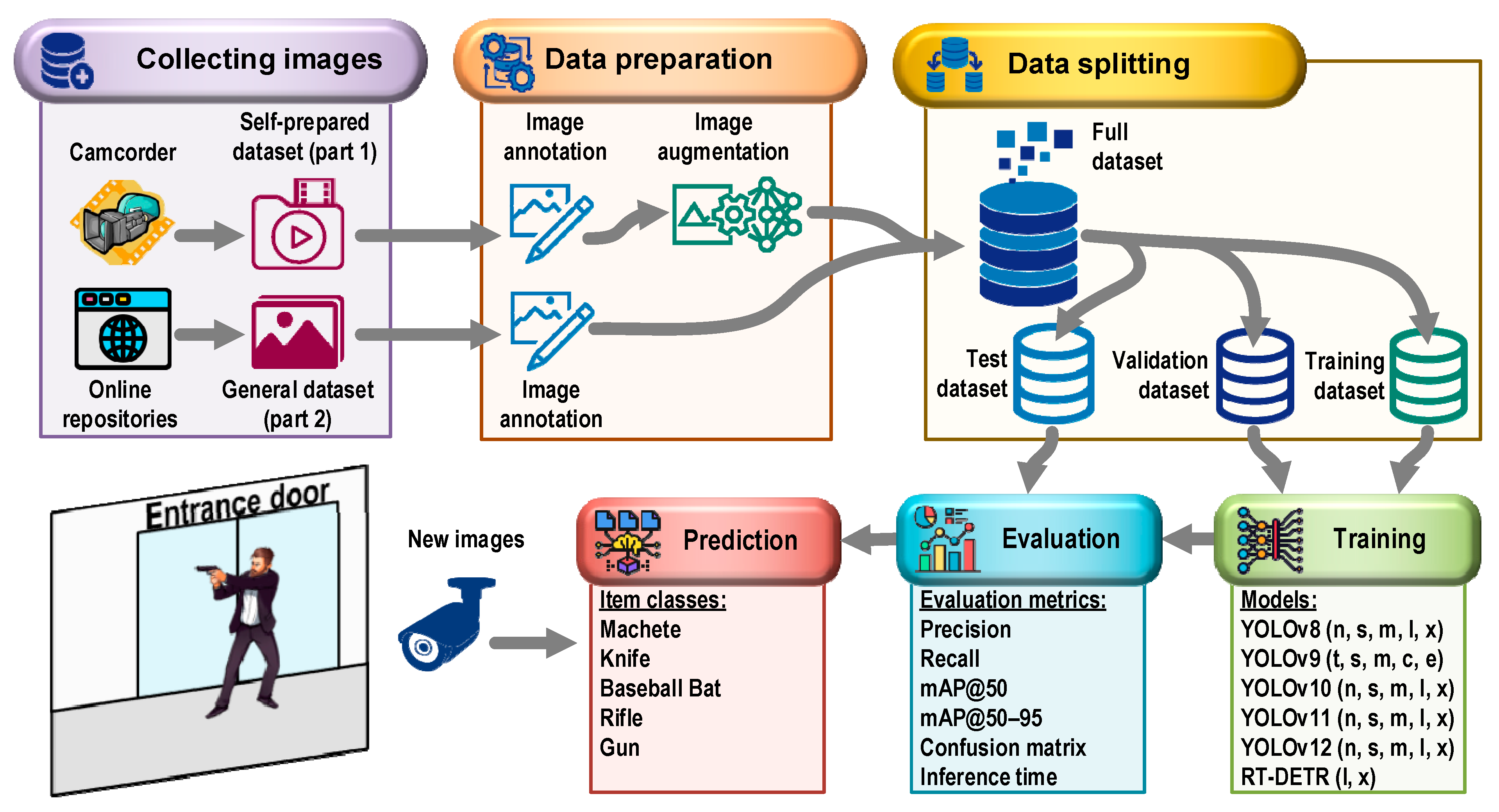
The process flow during the research is presented in Figure 2. The research material consisted of two parts. The first part was recorded independently using a video camera at the entrance to the monitored room. The second part of the images was collected using publicly available online repositories.
After labeling the collected images, the first part was additionally subjected to augmentation. After combining the augmentation results with the second part of the images, a complete dataset was obtained. Next, this set was randomly divided into training, validation, and test parts. The training and validation subsets were used to build models, and the test set was used to evaluate them. The best model, recommended for application, was used to predict new images when detecting dangerous items at the entrance to the monitored room.

2.1. Research Material

It is important to note that each item detector model is built for a specific application. This application determines the content of the training image set. If the detector is intended to detect dangerous items being brought into a building (e.g., a school), a sufficiently representative set of images presenting the detected items in this specific location must be collected. For this reason, a two-part dataset was used in this study. The first part was recorded independently near the entrance to the monitored room. The collected images presented 5 potentially dangerous items in various shots, such as a machete, knife, baseball bat, rifle, and gun. Images were recorded at 15 FPS using a Tracer HD WEB008 webcam (Megabajt Sp. z o.o., Warsaw, Poland) acting as a surveillance camera and a computer system with the following specification: a laptop with Windows 11 64-bit operating system, Intel Core i7-12650H 2.70 GHz processor, and 32 GB RAM. Every 30th frame was cut from the recorded video material, resulting in an extensive collection of images presenting various items. In the next step, the images were annotated in the YOLO standard using the Label Studio environment.
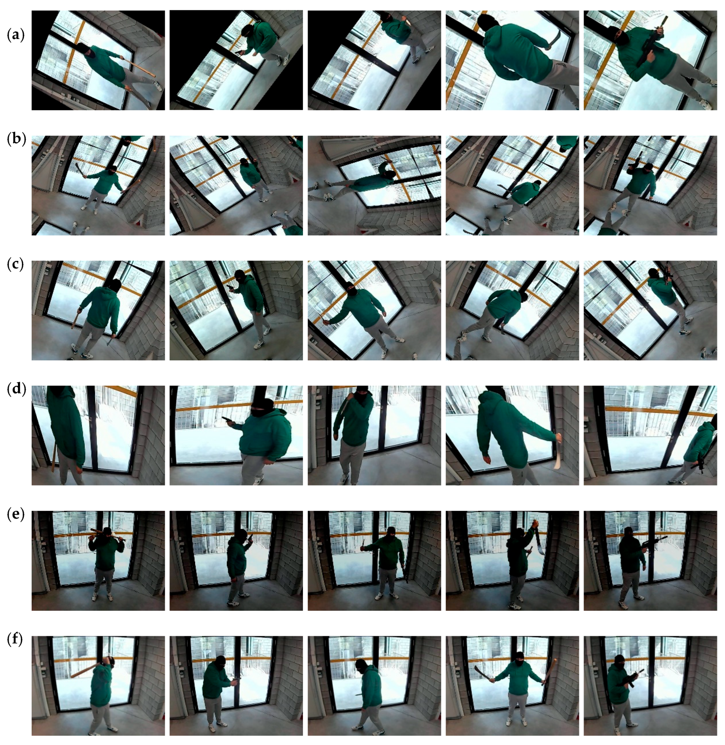
Next, these images were augmented using the Albumentations 1.3.1 package. As part of this process, the original dataset was expanded with images that could occur in real-world conditions. During augmentation, it is important to use transformations that do not lead to the creation of unclear images, i.e., those that confuse the model and increase the number of false positives. Therefore, appropriate parameter values for individual transformations were selected empirically. The transformations applied, the values of the parameters used, and examples of the transformation effects are presented in Table 2 and Figure 3. After augmentation, the size of the first part of the dataset was 4000 images.
The following functions were used during the transformation:
  • Affine—augmentation to apply affine transformations to images;
  • SafeRotate—rotate the input inside the frame by an angle selected randomly from the uniform distribution;
  • ShiftScaleRotate—randomly apply affine transforms: translate, scale, and rotate the input;
  • Perspective—apply random four-point perspective transformation to the input.
  • RandomBrightnessContrast—randomly changes the brightness and contrast of the input image;
  • GaussianBlur—apply Gaussian blur to the input image using a randomly sized kernel.
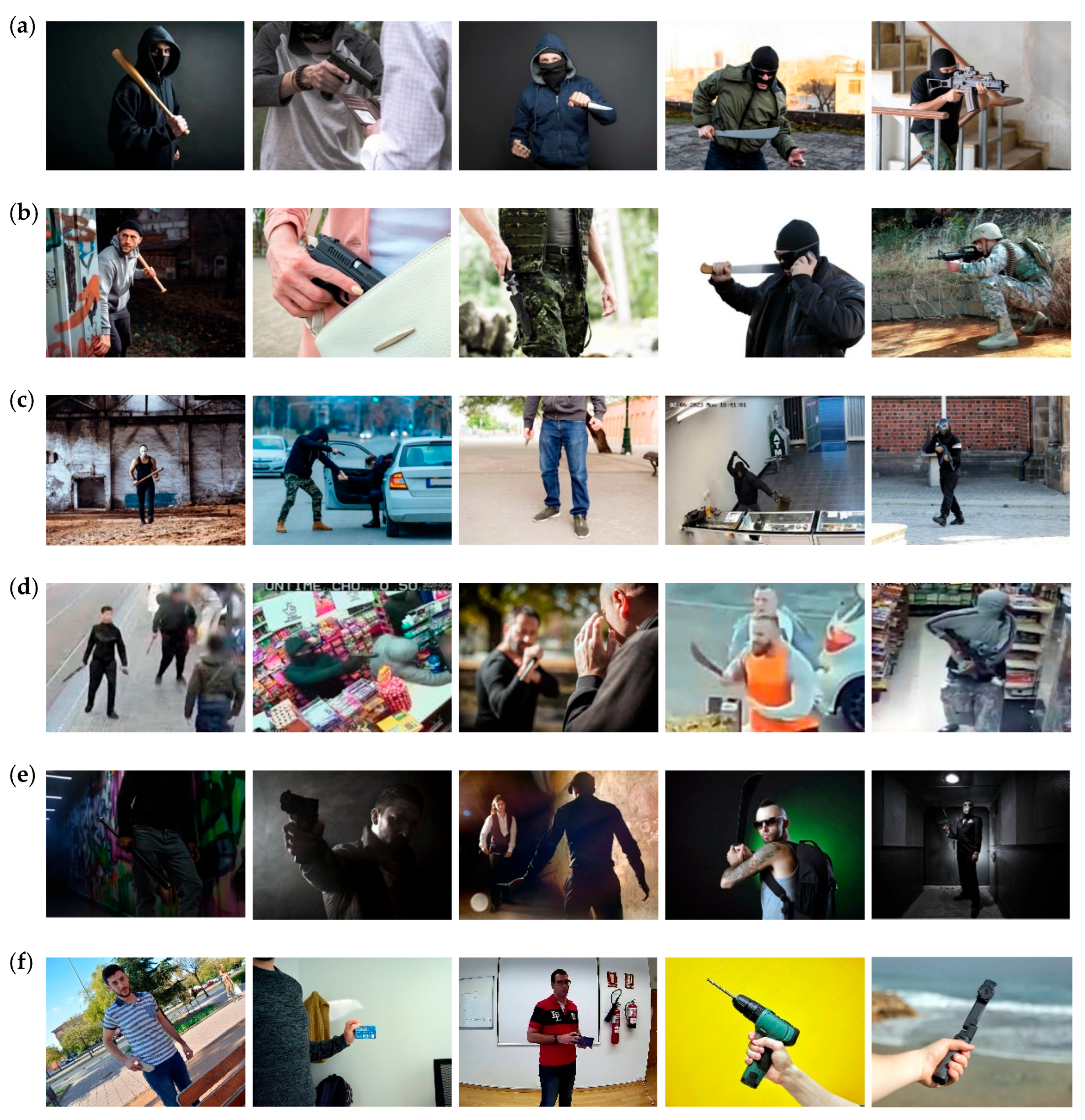
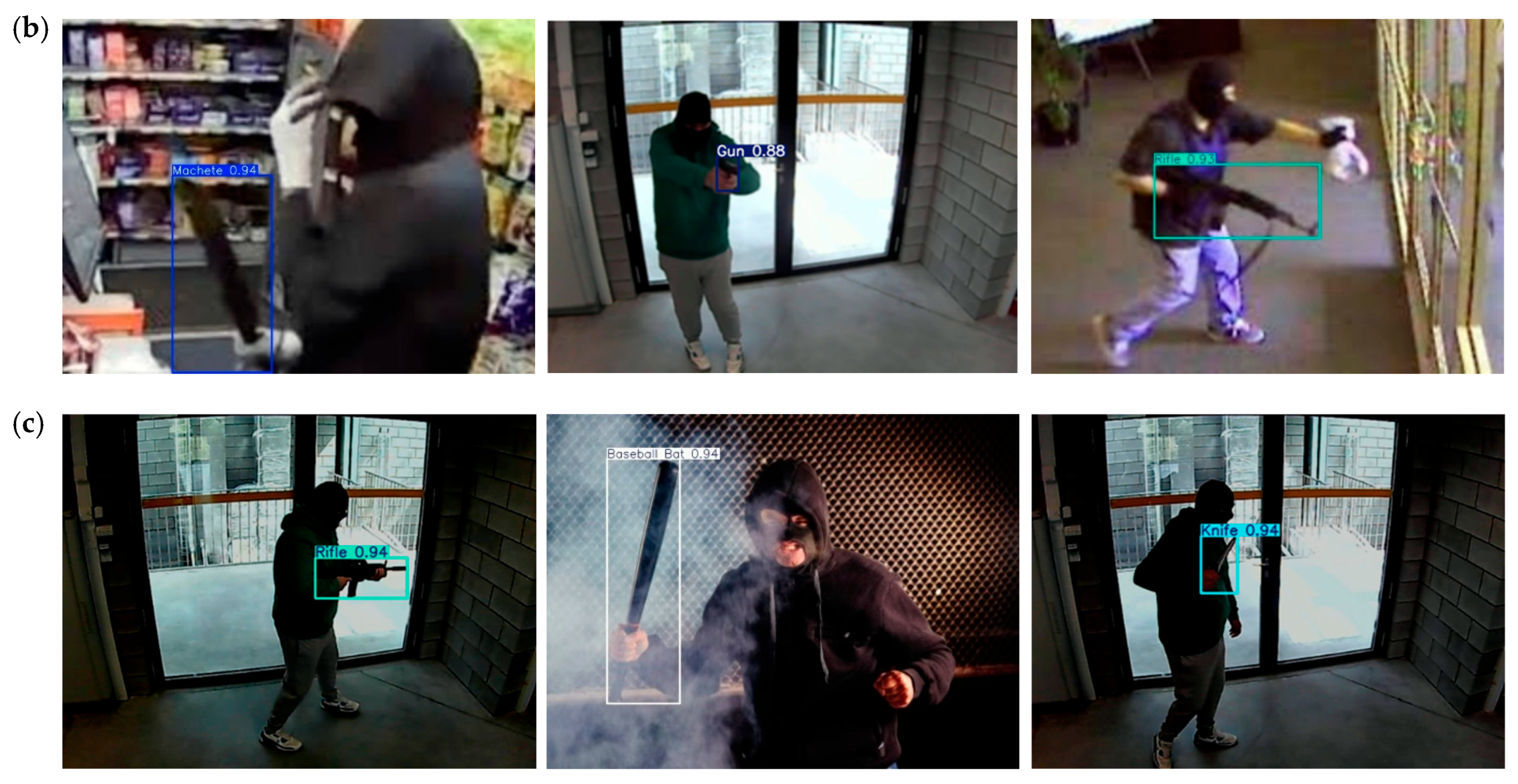
The second part of the dataset used to build the models consisted of 4478 images collected from publicly available online repositories. This part of the dataset presented detected items in various conditions and situations, which allowed for increasing the generalization capabilities of the built models. The dataset in question was built by the author as part of the research presented in [13]. It can be divided into several categories of images, examples of which are shown in Figure 4. These images were also annotated using the YOLO standard. The second part of the dataset also includes 826 background images, which are intended to reduce the number of false positive detections.
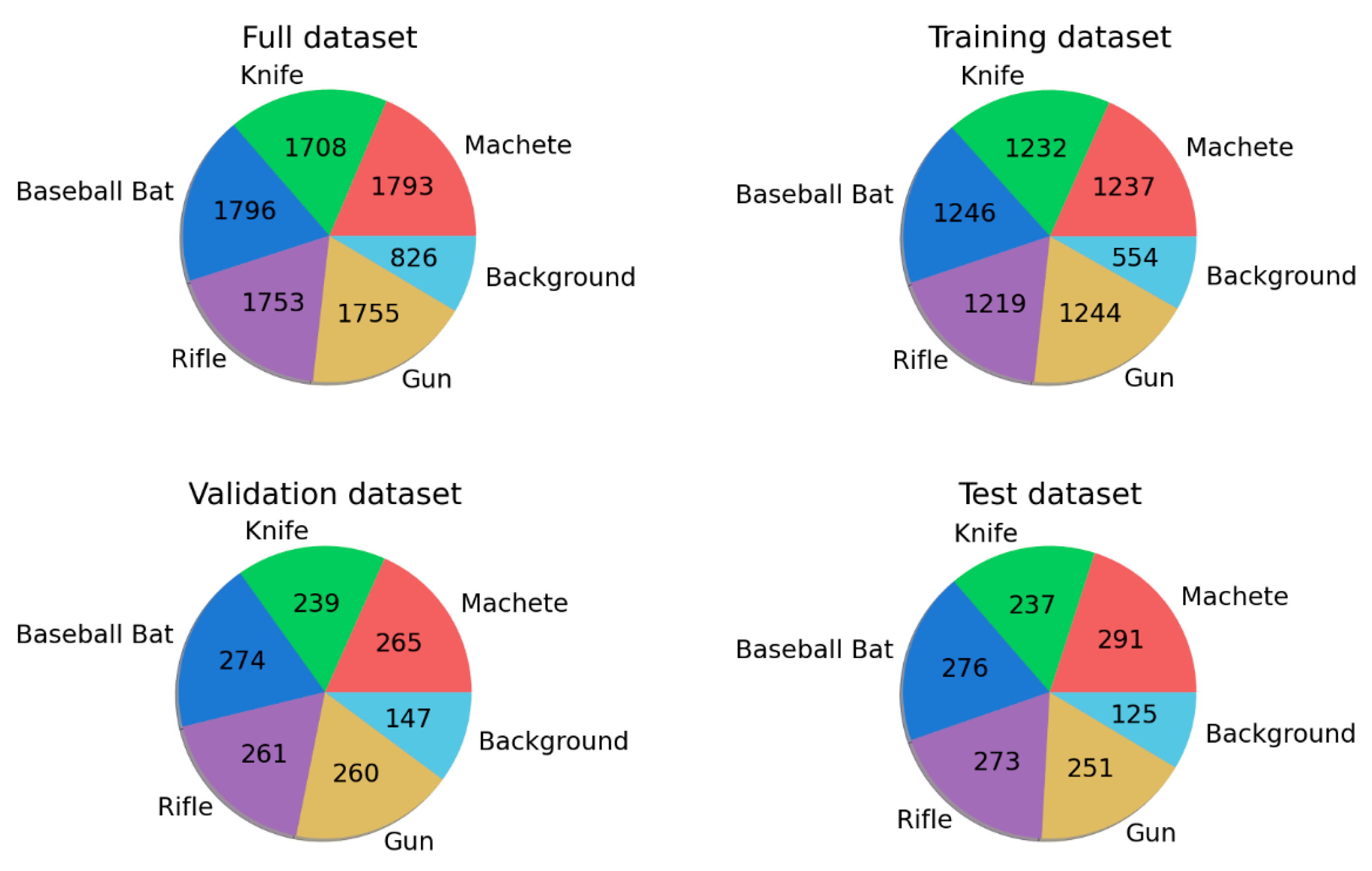
The complete dataset consisted of 8478 images and was created by combining 4000 self-collected images (part 1) and 4478 images downloaded from public datasets (part 2). The full dataset, which contained 8805 instances of detected items, was then randomly divided into training, validation, and test parts, in proportions of 70%, 15%, and 15% of the full set, respectively. As a result, the training set contained 5934 images, while the validation and test sets contained 1272 images each. The structure of these sets, specifying the number of detected items they contain, is shown in Figure 5. The dataset was made available on the Zenodo platform (https://zenodo.org/records/16422779, accessed on 3 September 2025).

2.2. The Idea Behind YOLO and Its Architectures

The latest architectures belonging to the YOLO and ViT families were used to build the models. The first model from the YOLO (You Only Look Once) family was described by J. Redmon [30]. Initially, the model divides the input image into a square grid of cells with dimensions S × S. Then, each cell predicts B bounding boxes. A given cell is responsible for detecting an object when the center of the object is located within it. Finally, the algorithm returns bounding boxes for which prediction confidence exceeds a set threshold and removes the rest using the Non-Maximum Suppression (NMS) algorithm.
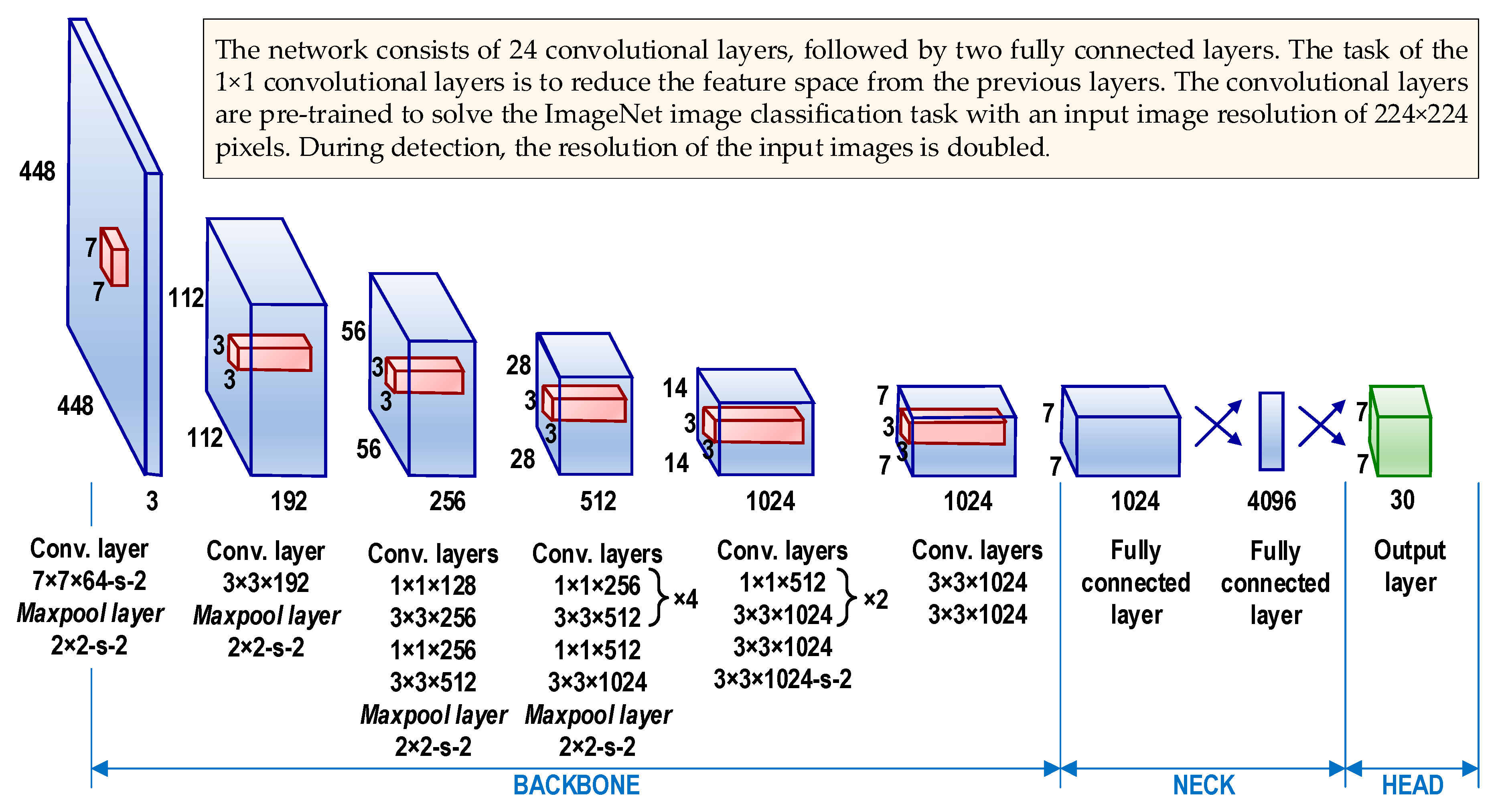
The YOLO model consists of three parts: the backbone, the neck, and the head. The backbone consists of convolutional layers used to detect key features of the image and process them. The model’s construction begins with the preliminary training of the network backbone using a dataset intended for image classification. The backbone is trained at a lower resolution than the final object detection model because detection requires more image details than classification. In the original YOLO model, the backbone was pre-trained on the ImageNet dataset containing images divided into 1000 classes. The Darknet framework was used for training [31]. The training includes 20 convolutional layers, followed by an average-pooling layer and a fully connected layer. During detection, four additional convolutional layers and two fully connected layers are added to the pre-trained network to increase the model’s performance (Figure 6).
Object detection, compared to classification, requires the presence of finer details in the image, which is why the resolution of input images is increased from 244 × 244 to 448 × 448 pixels during detection. The last layer, using a linear activation function, predicts the probabilities of class membership and the coordinates of the bounding box. To prevent overfitting, augmentation, and data dropout with a factor of 0.5 between the first and second fully connected layers were used.
The neck uses fully connected layers and, based on features derived from the backbone mesh layers, determines the prediction confidence and the coordinates of the bounding box. The head, on the other hand, is the output layer of the network, which can be interchanged with other layers with the same input shape to implement transfer learning. As stated in the source material, the head is formed by a tensor with the shape S × S × (B × 5 + C) [31]. The size of the grid into which the input image is divided is 7 × 7 (S = 7). The number of detected classes is 20 (C), and 2 bounding boxes (B) are predicted in each cell. It can therefore be seen that the final prediction is expressed by a tensor with a size of 7 × 7 × 30. The three parts of the model described above work together first to extract key visual features from the image and then classify and link them.

2.3. Modifications Introduced by Subsequent Versions of the YOLO and ViT Networks

The YOLO model was only able to predict two bounding boxes and one object class in a single grid cell. This limited the detector’s functionality when multiple small items belonging to different classes were in a single cell (e.g., different bird flocks). Therefore, in subsequent versions of the YOLO family of models, a number of modifications were introduced to improve their effectiveness and speed. The following section reviews the key changes introduced by subsequent versions of the YOLO family.
  • YOLOv2 [32]:
  • Darknet-19 backbone;
  • Anchor boxes (simplifying network learning);
  • Batch normalization (improved accuracy and model stability);
  • New loss function based on the sum of squares of errors between ground-truth and predicted bounding boxes (better suited for object detection tasks);
  • Replacement of fully connected layers with convolutional layers.
  • YOLOv3 [33]:
  • Darknet-53 backbone (improved accuracy);
  • Feature Pyramid Network (FPN) performing detection at 3 different scales (improved detection of objects of different sizes).
  • YOLOv4 [34]:
  • Cross Stage Partial Darknet-53 backbone (better performance while maintaining computational efficiency);
  • New method for generating anchor boxes (K-means clustering). The method clusters reference frames and then uses the group centroids as anchor boxes;
  • Gradient Harmonizing Mechanism loss function (improved model performance for unbalanced datasets);
  • Mosaic data augmentation (improved model generalization ability by introducing photometric and geometric distortions into the training set).
  • YOLOv5 [35]:
  • CSPDarknet-53 backbone;
  • Migration from the Darknet framework to PyTorch 1.6.0 (simplification of the implementation and experimentation process);
  • Mosaic data augmentation (increasing data diversity and improving small object detection by combining 4 training images into one);
  • Introduction of 5 model variants—nano, small, medium, large, xlarge (adaptation to different computational requirements).
  • YOLOv6 [36]:
  • EfficientNet-L2 backbone;
  • New method for generating anchor boxes, called dense anchor boxes.
  • YOLOv7 [37]:
  • Extended-ELAN backbone (increased learning and feature representation capabilities while maintaining gradient stability);
  • Use of 9 predefined anchor boxes for detecting objects of various shapes;
  • Use of Focal Loss;
  • Higher resolution of input images (608 × 608 pixels) than previous versions.
  • YOLOv8 [38]:
  • CSPDarknet-53 backbone;
  • Neck with dynamic label assignment (improved detection of objects of different scales);
  • Head without anchor boxes (better accuracy and more efficient object detection);
  • Advanced augmentation techniques, including image blending and affine transformations (increased resistance to interference).
  • YOLOv9 [39]:
  • Programmable Gradient Information technique—ensures that relevant data is retained in deep network layers, enabling the generation of reliable gradients that allow for accurate model updates and improved overall detection performance;
  • Generalized Efficient Layer Aggregation Network technique—allows for flexible integration of different computational blocks, enabling the model to be used in a wide range of applications without compromising speed or accuracy.
  • YOLOv10 [40]:
  • Use of an improved version of Cross Stage Partial Network as the backbone;
  • The neck aggregates feature from different scales using Path Aggregation Network;
  • Use of Dual-Head architecture:
    One-to-Many Head module—generates multiple predictions for each object, providing an adequate supply of training signals and improving learning accuracy.
    One-to-One Head module—generates a single, best prediction for each object. This eliminates the need for NMS, reduces latency, and improves performance.
  • YOLOv11 [41]:
  • Cross Stage Partial blocks with kernel size 2 (C3K2)—replace the previously used C2F blocks (improved processing speed while maintaining the ability to efficiently extract features);
  • Spatial Pyramid Pooling Fast (SPPF) blocks—ensure effective aggregation of multi-scale features (improved processing speed for objects of different sizes while maintaining high precision);
  • Parallel Spatial Attention (C2PSA) blocks—the parallel spatial attention mechanism allows the model to focus more precisely on relevant regions of the image (improved object detection accuracy).
  • YOLOv12 [42]:
  • A novel approach to the self-attention mechanism—feature maps are divided horizontally or vertically into regions of equal size—4 by default (avoiding complex operations and maintaining large effective receptive fields);
  • Improved feature aggregation module based on Residual Efficient Layer Aggregation Networks (meeting optimization challenges, especially in attention-focused models on a larger scale).
  • RT-DETR [43]:
  • Abandoning the NMS algorithm;
  • Using a belief-based framework;
  • Efficient hybrid encoder (the network achieves high real-time performance);
  • Separation of interactions between features within scales and combination of features between scales (efficient processing of multi-scale features);
  • Flexible inference speed adjustment using different decoder layers without the need for retraining.
There are many publications that provide an overview of the characteristics of individual versions of networks belonging to the YOLO family and compare them with each other [44,45,46,47,48].

2.4. Model Quality Assessment Measures

To evaluate the quality of the models, metrics using key concepts such as prediction confidence and intersection over union were used.
Prediction confidence—the probability estimated by the classifier that the predicted bounding box contains the object.
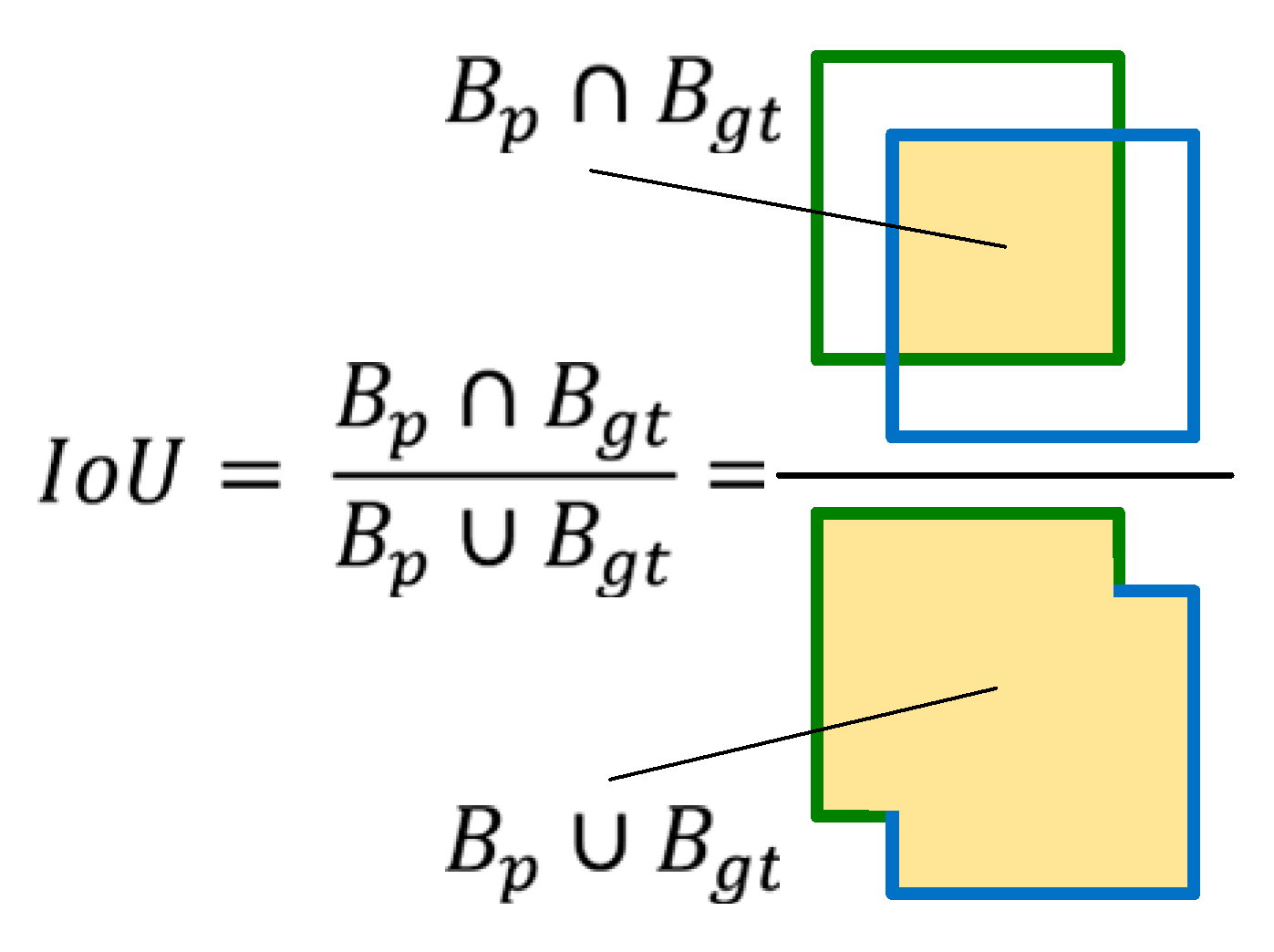
Intersection over union (IoU)—a measure that assesses the degree of overlap between the predicted box (Bp) and the ground-truth box (Bgt) (Figure 7).
Prediction confidence and IoU allow the following detection results to be determined:
  • True positive (TP)—occurs when the prediction confidence is greater than the accepted detection threshold (e.g., 0.5), the predicted class is the same as the class corresponding to the ground-truth box, and the predicted box has an IoU value greater than the detection threshold;
  • False positive (FP)—a false detection that occurs when either of the last two conditions is not met;
  • False negative (FN)—occurs when the prediction confidence is lower than the detection threshold (the ground-truth box was not detected).
Precision—the ability of the model to detect only correct objects, P r e c i s i o n = T P / ( T P + F P ) .
Recall—the ability of the model to detect all correct objects, R e c a l l = T P / ( T P + F N ) .
Average precision (AP)—the average of precision values corresponding to recall ranging from 0 to 1. Average precision is calculated separately for each class.
Mean average precision (mAP)—average precision calculated for all classes, m A P = i = 1 K A P i / K . Mean average precision can be calculated for different IoU thresholds, e.g., mAP@50 corresponds to the IoU threshold = 0.5. The mAP@50–95 measure is also used, which is calculated by averaging mAP for 10 IoU thresholds (0.50, 0.55, 0.60, …, 0.95).
Inference time—the time required for the model to make predictions about new, previously unknown data in a single image.
Frames per second (FPS)—the frequency at which inferences are made for successive frames of a video stream. The FPS value depends on the inference time and the duration of additional operations, such as image capture, pre-processing, post-processing, displaying results on the screen, etc.

3. Results

3.1. Training Process

During the model building and testing processes and the prediction of new images, the API provided by Ultralytics [49] was used. Table 3 provides a description and values of selected hyperparameters used during the model training and validation processes. The construction of the models was carried out on the NVIDIA DGX A100 computing platform, the main components of which were as follows: CPU—Dual AMD Rome 7742, 256 cores, 1 TB; GPU—8 x NVIDIA A100 SXM4 80 GB Tensor Core; OS: Ubuntu 22.04.5 LTS. The torch 2.3.0 platform and Python 3.10.12 programming language were used to build the models.
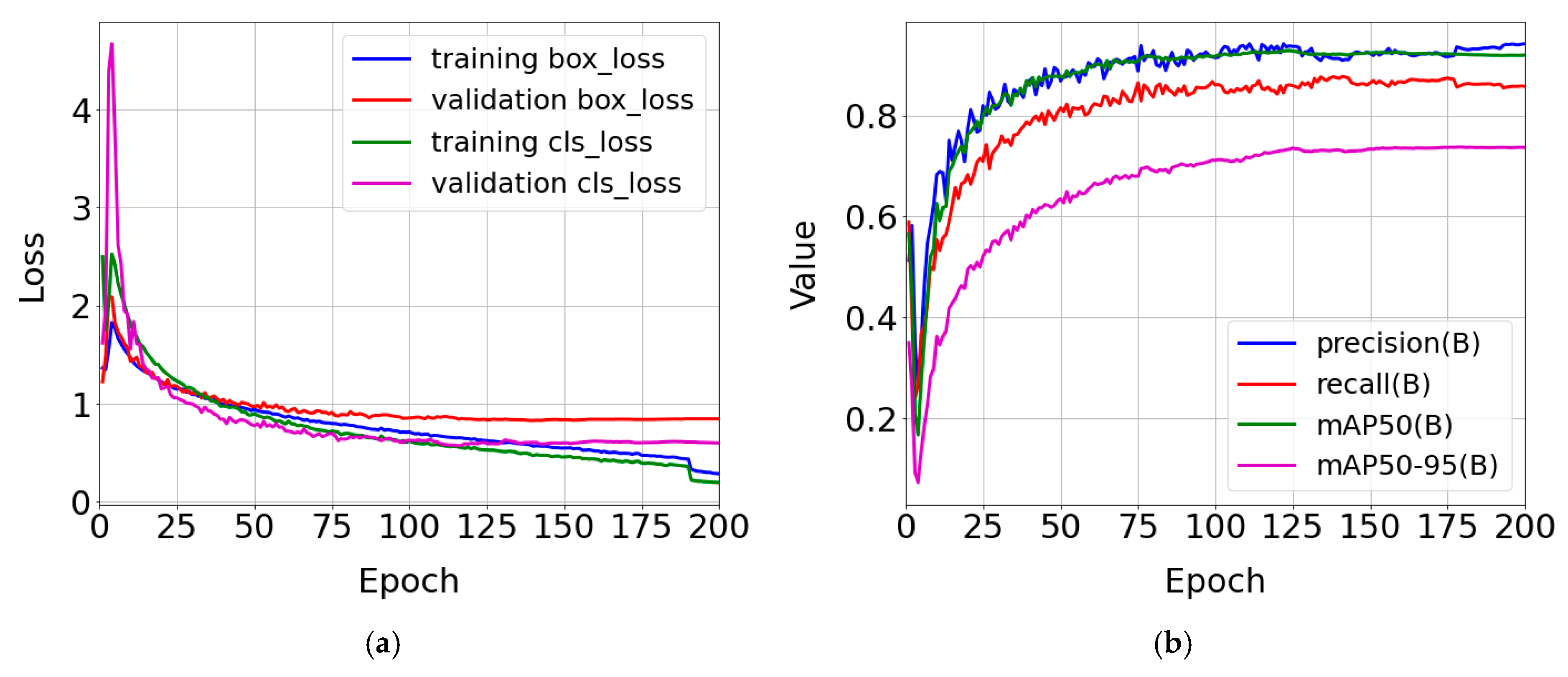
The study considered the latest versions of the YOLO network (YOLOv8-YOLOv12) and ViT architecture. Five models differing in the number of parameters for each YOLO network and two models for ViT (27 models in total) have been trained. Figure 8 shows example training and validation loss plots and basic detection quality metric plots for the validation set built for the YOLOv11m model.

3.2. Model Evaluation

After building the models, they were evaluated based on a test set. As a result of this process, information about the precision, recall, mAP@50, and mAP@50–95 of each model was obtained. A summary of the evaluation results is presented in Table 4. Based on these data, an analysis of the results was performed in the Discussion section to select the best model.

4. Discussion

4.1. Results Analysis and Selection of the Best Model

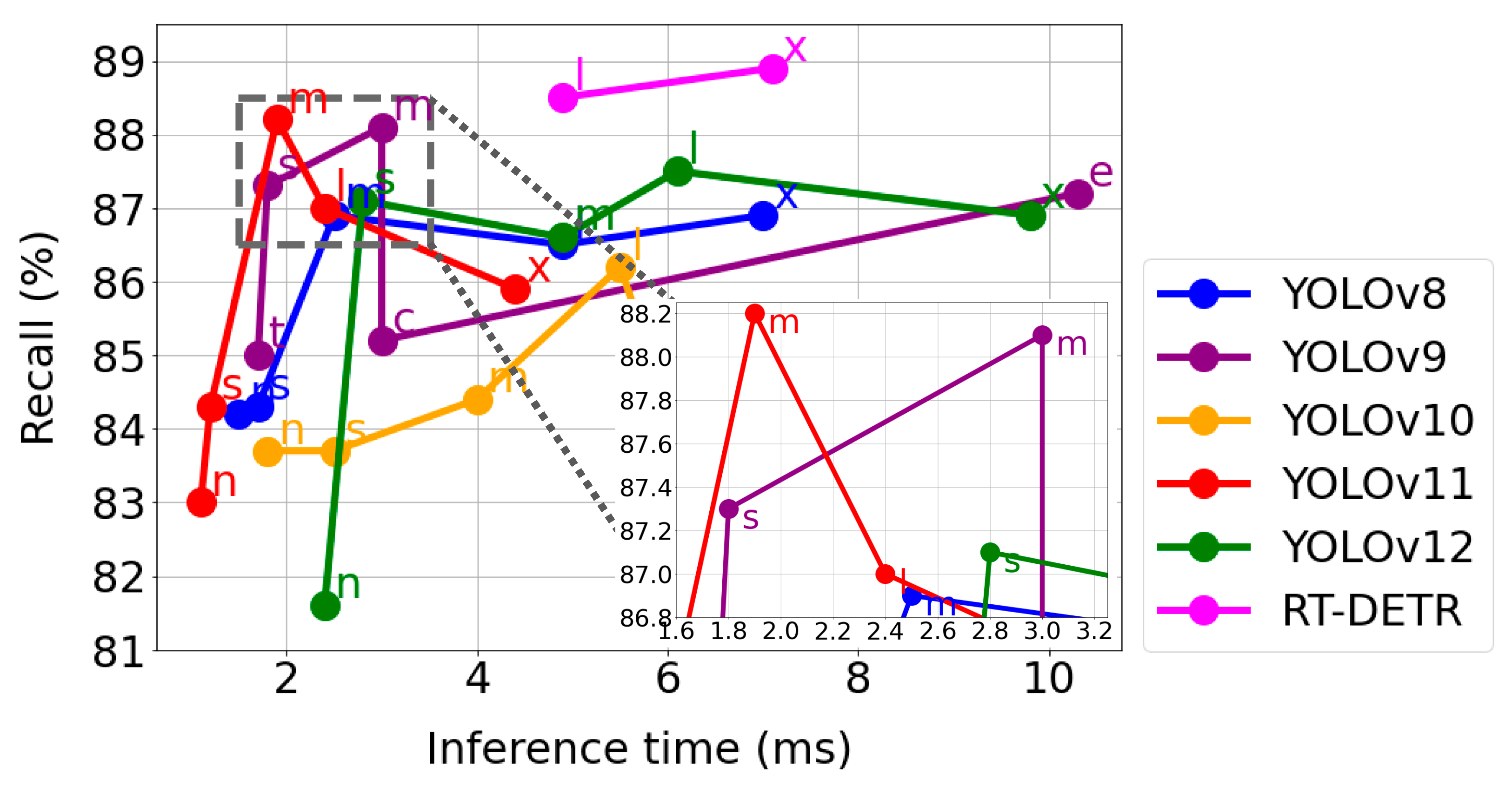
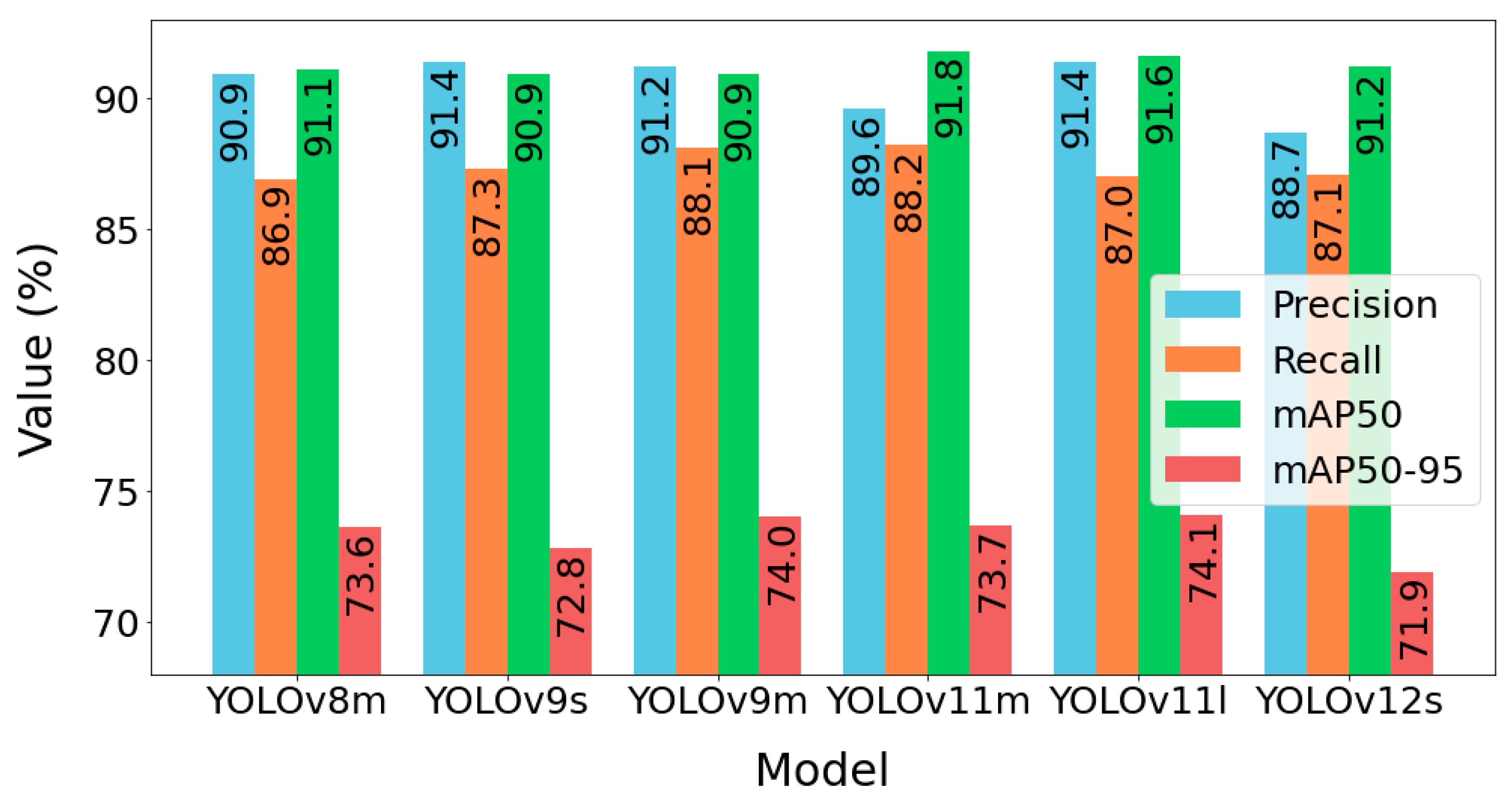
The key issue when choosing the best model is to determine the requirements it should meet. The model recommended on the basis of this research should, on the one hand, detect as many items of interest as possible appearing in the image (have high recall) and, on the other hand, perform the detection process in the shortest possible time (have a short inference time). The plot in Figure 9 provides a good overview of the defined criteria. The points visible in this graph represent pairs of values (recall, inference time) for individual models. Models that meet the predefined requirements are marked in Figure 9 with a gray dashed line, and the lower part of the graph shows an enlarged area of the range of values of interest (recall, inference time). On this basis, it is worth analyzing the properties of the following models in more detail: YOLOv8m, YOLOv9s, YOLOv9m, YOLOv11m, YOLOv11l, YOLOv12s. The performance parameters of these models, determined based on the test set, are presented in the form of bar charts in Figure 10.
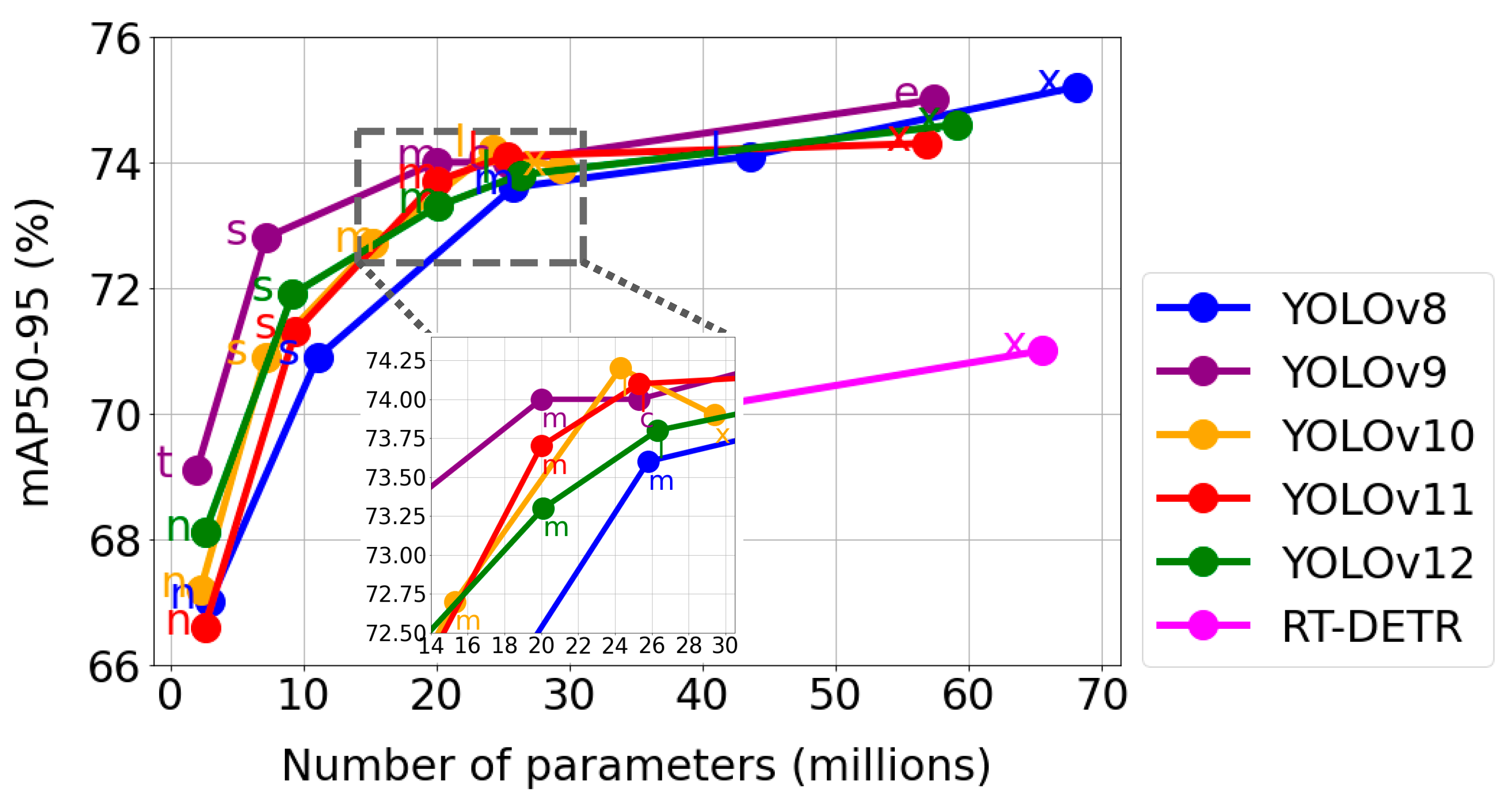
The second criterion for model selection is item detection precision, represented by the mAP@50–95 parameter. In Figure 11, the gray dashed line marks the area of pairs of values (mAP@50–95, complexity) that meet the requirement of a high mAP@50–-95 value and moderate model complexity. The selected area is shown in the lower part of Figure 11 in an enlarged view. Among the previously selected models, the second criterion is met by: YOLOv8m, YOLOv9m, YOLOv11m, and YOLOv11l.
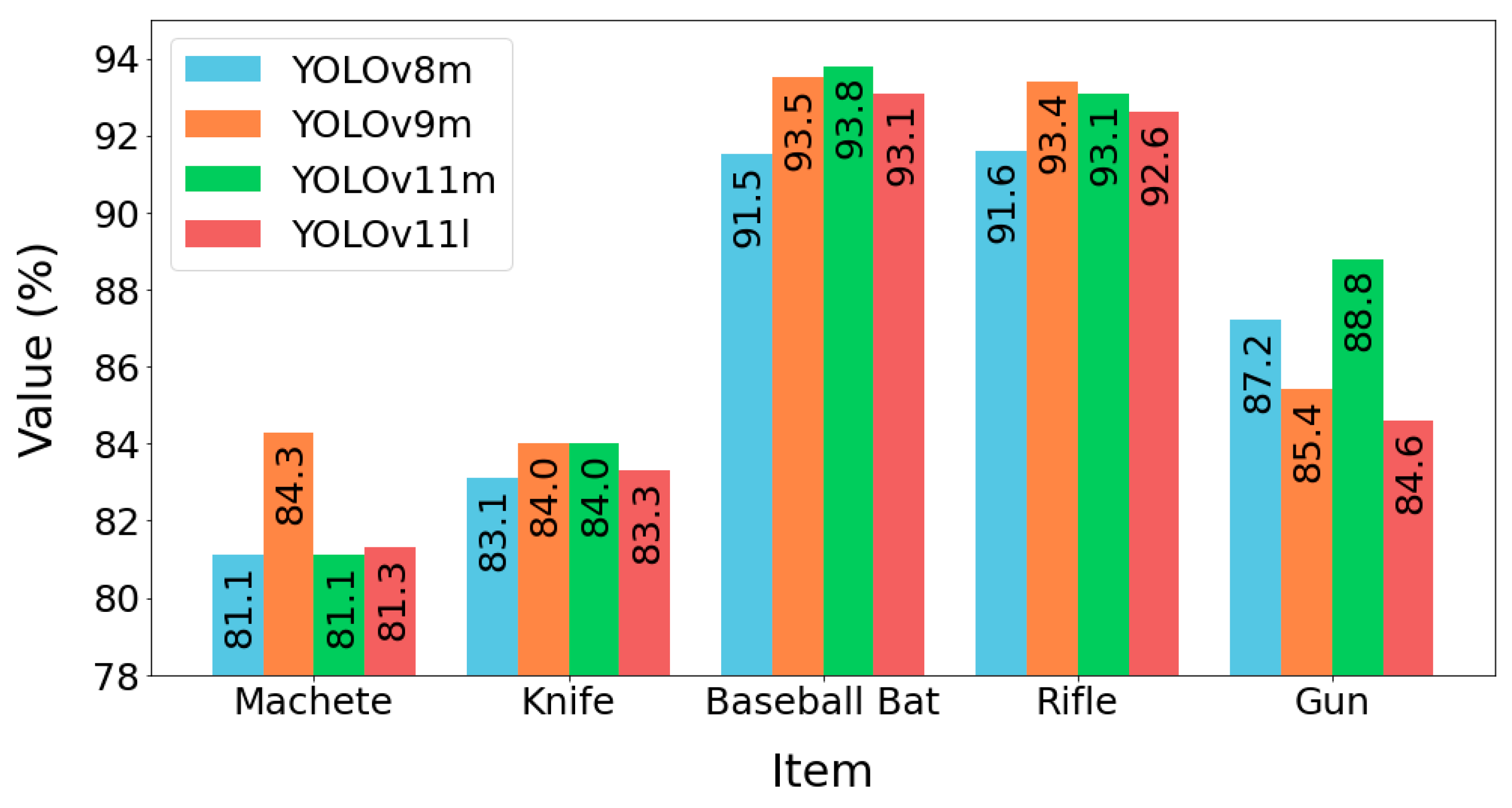
The detection recall of individual item classes determined based on the test set is presented in bar charts in Figure 12. The high effectiveness of the YOLOv11m model in detecting small items is noteworthy. This model achieved the highest detection recall for guns (88.8%) and knives (84.0%). As for the detection recall of other items, it was highest for baseball bats (93.8%), while for rifles, the recall achieved the second highest result—93.1%. In summary, it can be concluded that among the models analyzed in Figure 12, the YOLOv11m model proved to be the most effective for most of the detected items.
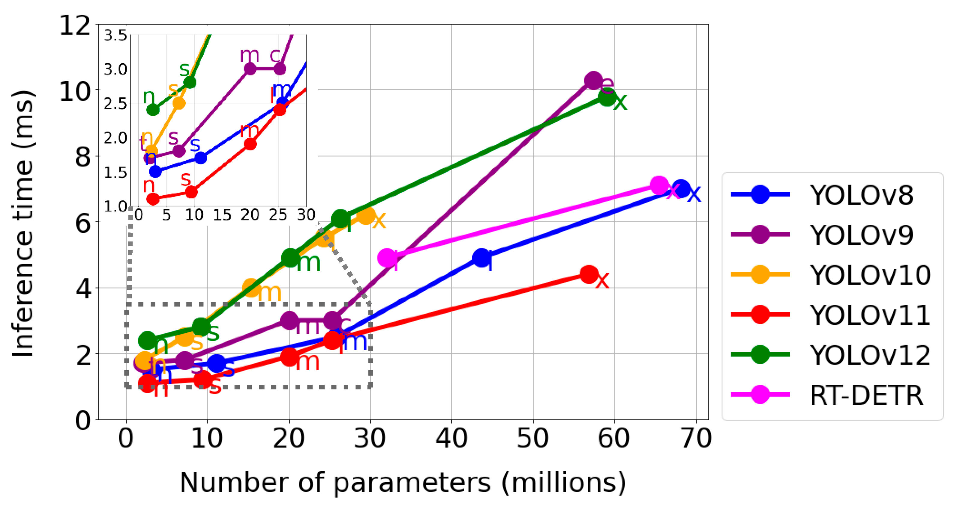
Figure 13 shows the inference time and complexity of individual models. The upper part of the graph shows an enlargement of the area of interest for parameter values. Of the four models indicated above, the YOLOv11m model has the most favorable parameter values. Its inference time is the shortest, at 1.9 ms, while the number of parameters in this model is approximately 20 million. It should be noted that the total image frame processing time (tproc) consists of three components: pre-processing (tpre), inference (tinfer), and post-processing (tpost) times. For the YOLOv11m model, these times were as follows: tproc = tpre + tinfer + tpost = 0.2 ms + 1.9 ms + 0.7 ms = 2.8 ms. This value gives a theoretical processing speed of 357 FPS. The actual processing speed is lower because there are additional delays associated with operations such as image capture, displaying results on the screen, etc. As a result, the FPS depends on the model architecture and the hardware and software platform on which the model is running.
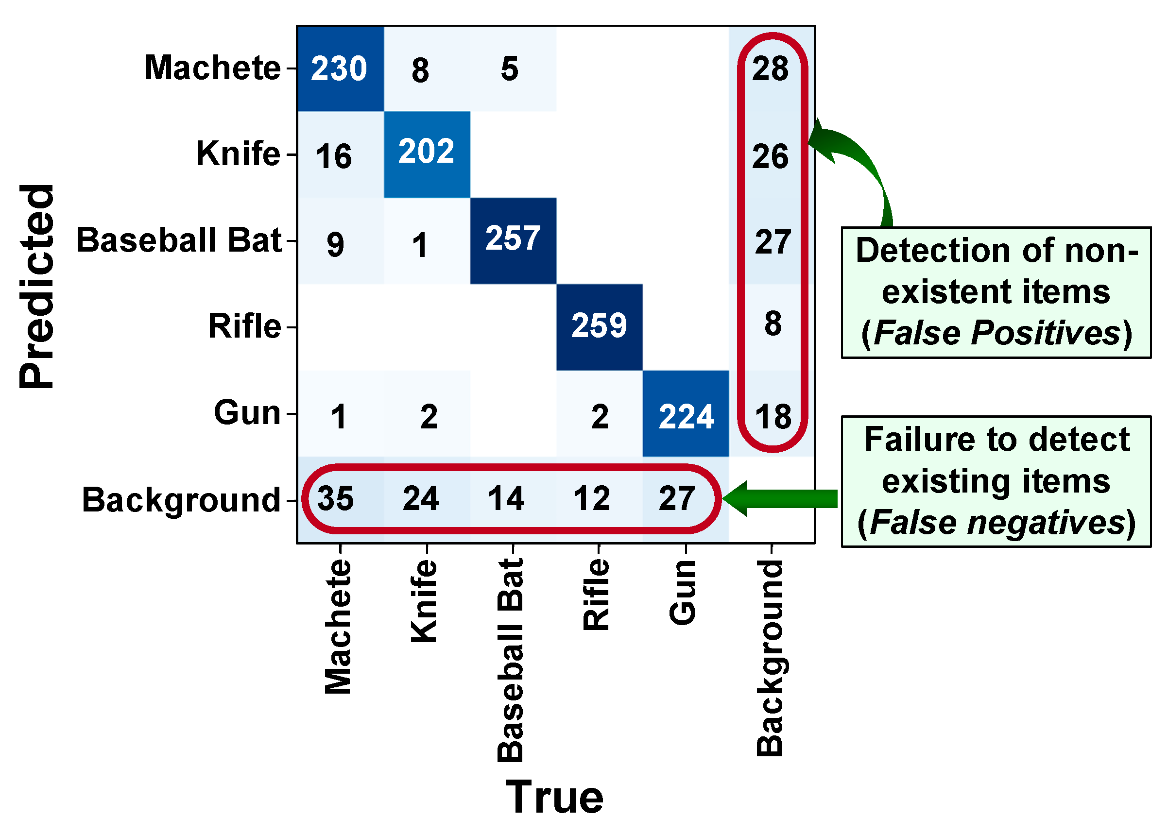
Figure 14 shows the confusion matrix constructed for the YOLOv11m model based on the test set. Due to the similarity in shape and often comparable length of the items, there were more mistakes between machetes and knives. In this case, 16 machetes were mistakenly identified as knives and 8 knives were detected as machetes. It should be noted that the primary goal of weapon type detection is to inform the appropriate authorities about the type of threat. Therefore, in future research, it is worth considering combining the two classes of machetes and knives into a single class, e.g., “edged weapons.” This could reduce the number of errors involving confusion between these two types of objects. The same reason (similar shape and length of items) was the source of a higher number of mistakes between machetes and baseball bats. In this situation, nine machetes were incorrectly detected as baseball bats, and five baseball bats were recognized as machetes. The number of errors concerning other items was negligible. However, there were quite a few false positive and false negative detections. False positives occurred when background items were recognized as dangerous ones. There are many ways to reduce the number of such cases. The most popular ones include: (1) improving the quality of training data—more negative data, better annotations, greater data diversity; (2) adjusting detection thresholds—confidence threshold, Non-Maximum Suppression threshold; (3) hard negative mining—improving model performance by focusing during training on the most difficult examples that have been incorrectly classified; (4) adjusting weights in the loss function—applying a greater penalty for false detections of a given class, the use of Focal Loss which helps the model focus on difficult examples, reducing FP; (5) data augmentation—using transformations that do not lead to the creation of unclear images that can confuse the model and increase FP. There were also a fairly large number of cases where dangerous items were not detected despite their presence in the image (false negative detections).
The largest number of such cases concerned machetes (35), as this item is impossible to detect if it is positioned with the blade facing the camera. There was also a problem with detecting small items such as knives and pistols, with 24 and 27 false negatives, respectively. Such item is difficult to detect when only a part of it is visible and the rest is hidden in the hand, or when the position of the item relative to the camera makes it difficult to recognize. The number of false negatives can be reduced by increasing the number of images in the training set that show the aforementioned items in positions that make them difficult to recognize. This refers to situations where machetes and knives are pointed toward the camera with their blades, and rifles and pistols are pointed toward the camera with their muzzles. Figure 15 shows an example of the prediction results made by the YOLOv11m model based on the test set.
The fact that the ViT models performed worse in this study compared to the YOLO models (e.g., considering the mAP@50–95) may be due to numerous factors. On the one hand, YOLO networks are more optimized for real-time object detection. They have a high-performance CNN-based architecture that works well with smaller datasets and is computationally optimized for fast inference. On the other hand, ViT technology, while effective for many vision-related tasks, may not work as well for object detection (especially for smaller datasets like the one used in the research) due to its reliance on transformers, which are computationally expensive, process a lot of data, and do not have as efficient mechanisms for handling spatial dependencies, that occur in YOLO networks. Thus, it can be concluded that YOLO networks can outperform ViT in object detection, especially in real-time, low-resource, or smaller-data environments, while ViT may be better suited for tasks where there are long-term dependencies or for large, high-quality datasets.

4.2. Comparison of Results with Those of Other Authors

Table 5 summarizes the results of dangerous item detection obtained by other authors. The first 10 rows of this table present the results obtained using YOLO networks. First, it should be noted that most studies conducted using these networks focus on the detection of firearms, especially guns. The best detection recall for this type of item was achieved by Ashraf et al. (99%) [50], followed by Shanthi et al. (95%) [51], and in third place by Yadav et al. (91.4%) [52]. The recall obtained in this study (88.8%) is lower than those mentioned above, but it is still high and exceeds the results obtained by other authors listed in Table 5. The precision of gun detection obtained by other authors exceeds 90% in most cases, with the best result obtained by Bushra et al. being 98% [53]. The author’s own result, equal to 90.5%, is lower, but nevertheless satisfactory and exceeds the results of other authors. As for the precision of knife detection, Sun et al. obtained a result of 57.2% [54]. Own results in this case are significantly higher, at 84.4%. Unfortunately, there are no results available to compare the detection recall of other types of dangerous items, such as machetes, baseball bats, and rifles. Comparing mAP values is not easy, as it determines the average precision for all detected classes. Against this background, own dataset is more complex, as it contains five classes of different items. In contrast, the datasets used by other authors are simpler and more limited in this respect, as they usually contain only guns or only several types of firearms. Furthermore, the datasets used by other authors are often limited in number, and the authors do not provide information on the quality of the images they use (blurring, poor lighting, small items, etc.). In this context, own mAP result (91.8%) seems particularly good.
The second part of Table 5 (last 10 rows) shows the results obtained using Faster R-CNN networks. They are very popular for detecting dangerous items due to their high accuracy in detecting small items. The largest number of available results concerns the detection of guns; according to statistics, this is the most used weapon in robberies and acts of violence. The precision value obtained for this case (90.5%) is lower than the precision achieved by Vijayakumar et al. (96.6%), but the dataset used by the authors leaves much to be desired [62]. They do not provide information on the number of instances of each class. According to the data, the full set contained only 120 images of guns, of which 96 were used for training and 24 for testing. In addition, a significant proportion of the images (60%) showed guns without a real background, and only 40% showed them in real conditions (held in a hand). Both the number and structure of the image set give reason to suspect that the result obtained is overestimated. In terms of gun detection recall, the best result (100%) was achieved by Olmos et al. [61] and González et al. [65]. Own result (88.8%) ranks third. It is difficult to compare these results because Olmos et al. and González et al. achieved 100% sensitivity for binary models designed to detect only guns (or guns and rifles), while the model used in own research is multi-class (it detects 5 classes of items). In this situation, sensitivity of 88.8% should be considered high. Significantly fewer results are available for rifle detection. The rifle detection precision of 95.1% obtained in own research is the second best in the presented comparison. The best precision (100%) was achieved by Vijayakumar et al. [62]. However, the accuracy value reported by the authors is overestimated due to the limited dataset. The full collection contained only 135 images of rifles, of which 108 were used for training and 27 for testing. For comparison, the set used in this study contained 1753 rifles (training set—1219, validation set—261, test set—273). The recall of rifle detection in this study was 93.1%. Vijayakumar et al. achieved a higher recall of 96% in this case [62]. However, this result is not very reliable due to the size of the dataset used (as in the case of precision). In terms of knife detection precision, the best result was achieved (84.4%). It is significantly better than the results obtained by other authors, which were 80.8% (Omiotek [13]), 55.8% (Vijayakumar et al. [62]), and 46.7% (Fernandez-Carrobles et al. [65]). The second-best result in terms of knife detection recall (84%) was obtained in own research. The highest result was obtained by Omiotek and amounted to 90% [13]. Apart from the results of Omiotek [13], any research results on the use of Faster R-CNN for detecting baseball bats and machetes were unable to be found. This proves the unique nature of the dataset used in this study and the results obtained. As for the mAP parameter, which describes the average detection precision of all item classes, the obtained value (91.8%) exceeds all results obtained for the Faster R-CNN.

4.3. Testing the Model Using New Images

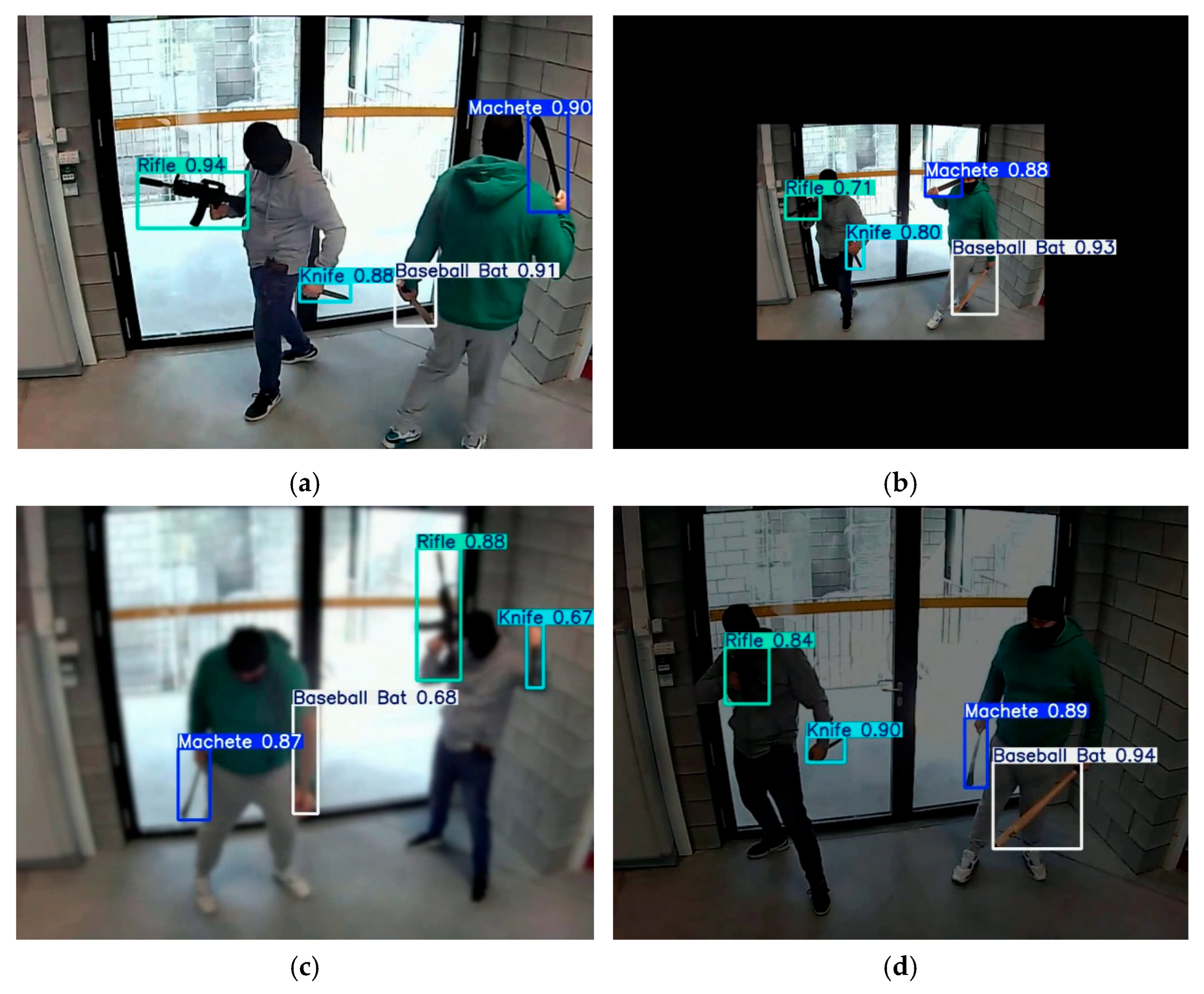
The model considered to be the most effective (YOLOv11m) was tested under the same conditions as those in which the first part of the test set was recorded. Figure 16 presents selected prediction results obtained under different environmental conditions.
In normal visibility conditions, all items were detected correctly. Similar high model effectiveness was observed when the image size was reduced by 50% (smaller items). In the case of poorer image sharpness, larger items (rifle, baseball bat, machete) were detected quite well, while there were problems with detecting smaller items (knife). Finally, with reduced lighting (darker items), the effectiveness of item detection was like before. During the tests, there were periods when a given item (especially a small one, such as a knife) was not detected, but these were so short that they did not affect the high rating of the effectiveness of detecting the presented items. The images were recorded at a resolution of 1000 × 750 pixels using the same computer system that was used to collect the first part of the dataset. The technical parameters of this system allowed for smooth display of prediction results at a speed of up to approximately 60 FPS. This situation shows that the YOLOv11m model can be easily integrated into typical general-purpose computer systems. Selected excerpts from the course of the experiment are shown in a video made available on the Zenodo platform (https://doi.org/10.5281/zenodo.16498782).

4.4. Model Limitations

Based on the research and test results, the YOLOv11m model was rated the best. However, like other object detection models, it also has certain limitations. The following section highlights potential problems that should be considered:
  • The problem of accuracy and generalization. The model was trained on a limited set of dangerous items, so its accuracy may be lower for new, unknown images presenting other forms of the same items. The significance of this problem was reduced during the research by using the second part of the dataset, which was designed to increase the generalization properties of the model. The tests showed 112 false negatives (8.4%) and 107 false positives (8%). The number of false negatives can be reduced by expanding the training set with a larger number of images depicting certain objects in positions that make them difficult to recognize. For example, machetes and knives are pointed toward the camera with their blades, and rifles and guns are pointed toward the camera with their barrels. Similarly, the number of images depicting objects that are partially covered should be increased. The model had the most difficulty recognizing machetes and knives because when they are pointed toward the camera lens, these objects look similar. In addition, in both cases, there may be items that are comparable in shape and length. The severity of this problem can be reduced by increasing the number of images in the training set that show machetes and knives in shots that are difficult to recognize;
  • Limited understanding of context. Models based on local characteristics ignore the surrounding context, which may be important for detection accuracy. For example, detecting a knife at a school entrance will be treated the same as detecting a knife in a kitchen. There are no ideal models that are universal for every application. In this study, it was emphasized that the purpose of the model is to detect dangerous items before entering a monitored room (e.g., a school). Therefore, an extensive set of training images (part 1) was used to teach the model to understand this specific environmental context;
  • Sensitivity to input data. Model tests conducted in various environmental conditions revealed problems with detecting small objects (knife, gun) in cases of poorer image sharpness and lower light intensity. To mitigate this problem, various categories of training images were used (items clearly visible, partially covered, small items, poor image sharpness, poor image illumination, and background images). Further steps may involve the use of image preprocessing algorithms before sending images to the model input;
  • Difficult detection of small and overlapping objects. The model detects small objects less well than large ones. The number of undetected knives and guns was more than twice the number of undetected baseball bats and rifles. The problem of detecting small objects remains a challenge in the field of computer vision. One way to solve this problem is to increase the number of small objects in the training set. It is also possible to use a network that is more accurate at detecting small objects, such as Faster R-CNN, at the cost of increased inference time;
  • Limited number of categories. The model has been trained to detect only five potentially dangerous items (machete, knife, baseball bat, rifle, and gun). In real-world conditions, other objects may serve as “dangerous” items. Therefore, the model should be retrained to include items that should be detected in specific conditions and applications of the model;
  • Implementation limitations. The model tests were performed on a computer with the following hardware specifications, which set the general framework for implementation: Intel Core i7-12650H 2.70 GHz processor, 32 GB RAM, and NVIDIA GeForce RTX 3060 GPU with 6 GB GDDR6. In addition, the following software components were installed: python 3.10.15, opencv-python 4.11.0.86, torch 2.5.1+cu118, ultralytics 8.3.75. The above specification allowed for smooth display of forecasting results at a speed of up to approximately 60 frames per second. In summary, it can be concluded that the model does not have excessive requirements in terms of computer system technical parameters and can be easily integrated with typical general purpose computers. It should be added here that it is not possible to directly implement the model on edge devices. In this case, appropriate model optimization is required.

4.5. Potential Application of the Built Model

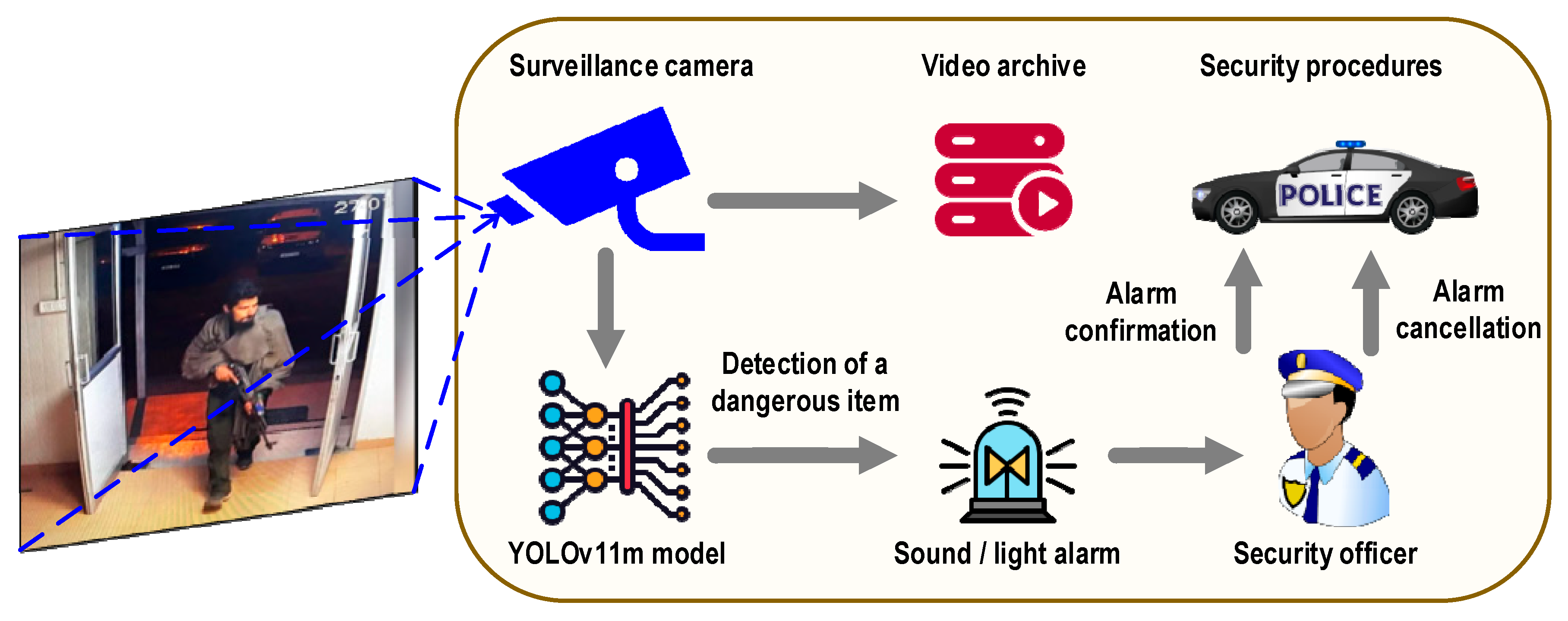
One possible way in which a system implementing a machine learning model might operate is shown in Figure 17. If a dangerous item, learned by the model, is detected in the camera’s field of view, the system will mark it on the image and automatically generate detection information in a manner specified by the user. This can be a light or sound signal emitted in the control room, allowing the employee responsible for monitoring the video surveillance system to more accurately assess the threat and decide on further steps related to safety. If the alarm is confirmed, appropriate security procedures can be implemented, such as announcing an alarm throughout the building, informing security services, evacuating the facility, locking doors, or tracking the attacker. Thanks to the integration of the dangerous item detector with the existing monitoring system, threats within the camera’s field of view can be detected even if they are visible for only a short period of time. This is a significant improvement, as it not only increases the comfort of video system controllers, but also provides additional protection against potential human error in the form of overlooking essential information. This solution takes away unnecessary pressure on security personnel, allowing them to focus on other tasks, and reduces the number of staff required.

5. Conclusions

During this research, the effectiveness of modern models from the YOLO and ViT architectures in detecting dangerous items in various image acquisition conditions was evaluated. The most effective model was YOLOv11m, which achieved the following detection quality metrics (for all classes): Recall = 88.2%, Precision = 89.6%, mAP@50 = 91.8%, mAP@50–95 = 73.7%. These are satisfactory results, considering the complexity of the dataset used. The dataset consisted (in similar proportions) of images in which the detected items were clearly visible, partially obscured, small, blurred, and poorly visible. These image characteristics increased the difficulty of the item detection task. Evaluation on the test set and prediction of new images using a typical webcam showed that the YOLOv11m model performs very well in detecting dangerous items regardless of the input image quality. The theoretical frame processing speed for this model was 357 FPS, while the actual speed, using a typical general-purpose computer system, reached 60 FPS. These results allow us to recommend the YOLOv11m model for use in public monitoring systems designed to detect specific items (e.g., potentially dangerous ones) brought by people into various facilities. The research used a strictly defined set of items (machete, knife, baseball bat, rifle, gun), but in accordance with the purpose of the surveillance system, this set can be expanded or modified as appropriate.

Funding

This research was funded by the Ministry of Education and Science—Poland, grant number FD-20/EE-2/315.

Data Availability Statement

The dataset used in the research is publicly available on Zenodo. DOI: 10.5281/zenodo.16422778.

Conflicts of Interest

The author declares no conflicts of interest.

References

  1. The Gun Violence Archive. Available online: https://www.gunviolencearchive.org/ (accessed on 18 June 2025).
  2. Jang, S.; Battulga, L.; Nasridinov, A. Detection of Dangerous Situations using Deep Learning Model with Relational Inference. J. Multimed. Inf. Syst. 2020, 7, 205–214. [Google Scholar] [CrossRef]
  3. Triguero, F.; Tabik, S.; Lamas, A.; Hernández, F.; Pimentel, R. Weapons detection for security and video surveillance. Pattern Recognit. 2024, 147, 109192. [Google Scholar]
  4. Ha, E.; Kim, H.; Na, D. HOD: New harmful object detection benchmarks for robust surveillance. Comput. Vis. Image Underst. 2024, 238, 103059. [Google Scholar]
  5. Pérez-Hernández, F.; Tabik, S.; Lamas, A.; Olmos, R.; Fujita, H.; Herrera, F. Object Detection Binary Classifiers methodology based on deep learning to identify small objects handled similarly: Application in video surveillance. Knowl. Based Syst. 2020, 194, 105590. [Google Scholar] [CrossRef]
  6. Castillo, A.; Tabik, S.; Pérez, F.; Olmos, R.; Herrera, F. Brightness guided preprocessing for automatic cold steel weapon detection in surveillance videos with deep learning. Neurocomputing 2019, 330, 151–161. [Google Scholar] [CrossRef]
  7. Yadav, P.; Gupta, N.; Sharma, P.K. A Comprehensive Study towards High-level Approaches for Weapon Detection using Classical Machine Learning and Deep Learning Methods. Expert Syst. Appl. 2023, 212, 118698. [Google Scholar] [CrossRef]
  8. Gawade, S.; Vidhya, R.; Radhika, R. Automatic Weapon Detection for surveillance applications. In Proceedings of the International Conference on Innovative Computing & Communication (ICICC-2022), Delhi, India, 19–20 February 2022. [Google Scholar]
  9. Dugyala, R.; Reddy, M.V.V.; Reddy, C.T.; Vijendar, G. Weapon Detection in Surveillance Videos Using YOLOv8 and PELSF-DCNN. In Proceedings of the 4th International Conference on Design and Manufacturing Aspects for Sustainable Energy (ICMED-ICMPC 2023), Hyderabad, India, 19–20 May 2023. [Google Scholar]
  10. Azarov, I.; Gnatyuk, S.; Aleksander, M.; Azarov, I.; Mukasheva, A. Real-time ML Algorithms for the Detection of Dangerous Objects in Critical Infrastructures. In Proceedings of the 4th International Workshop on Intelligent Information Technologies and Systems of Information Security, Online Conference, 22–24 March 2023. [Google Scholar]
  11. Gao, Q.; Li, Z.; Pan, J. A Convolutional Neural Network for Airport Security Inspection of Dangerous Goods. IOP Conf. Ser. Earth Environ. Sci. 2019, 252, 042042. [Google Scholar] [CrossRef]
  12. Andriyanov, N. Deep Learning for Detecting Dangerous Objects in X-rays of Luggage. Eng. Proc. 2023, 33, 20. [Google Scholar]
  13. Omiotek, Z. Dangerous items’ detection in surveillance camera images using Faster R-CNN. Prz. Elektrotech. 2025, 101, 156–168. [Google Scholar] [CrossRef]
  14. Pistols Dataset. Available online: https://universe.roboflow.com/joseph-nelson/pistols (accessed on 30 August 2025).
  15. OD WeaponDetection. Available online: https://github.com/brooksideas/OD-weapon-detection-dataset?tab=readme-ov-file (accessed on 30 August 2025).
  16. Weapon Detection Dataset. Available online: https://www.kaggle.com/datasets/snehilsanyal/weapon-detection-test (accessed on 30 August 2025).
  17. Gun Detection Datasets. Available online: https://www.linksprite.com/gun-detection-datasets/ (accessed on 30 August 2025).
  18. Pistols YoloV5 Object Detection Dataset. Available online: https://universe.roboflow.com/weapons/pistols-yolov5-vlhoz/dataset/1 (accessed on 30 August 2025).
  19. Pistol Labeled Image Dataset. Available online: https://images.cv/dataset/pistol-image-classification-dataset (accessed on 30 August 2025).
  20. Weapons Labeled Image Dataset. Available online: https://images.cv/dataset/weapons-image-classification-dataset (accessed on 30 August 2025).
  21. Weapons in Images. Available online: https://datasetninja.com/weapons-in-images (accessed on 30 August 2025).
  22. Weapon Detection Dataset. Available online: https://www.kaggle.com/datasets/abhishek4273/gun-detection-dataset (accessed on 30 August 2025).
  23. Weapon Detection System. Available online: https://github.com/HeeebsInc/WeaponDetection (accessed on 30 August 2025).
  24. Mock Attack Dataset. Available online: https://github.com/Deepknowledge-US/US-Real-time-gun-detection-in-CCTV-An-open-problem-dataset (accessed on 30 August 2025).
  25. Gun and Knife Detection. Available online: https://universe.roboflow.com/mahad-ahmed/gun-and-knife-detection/dataset/1 (accessed on 30 August 2025).
  26. Pistol & Rifle & Knife Dataset. Available online: https://universe.roboflow.com/pistolrifle/pistol-rifle-knife/dataset/1 (accessed on 30 August 2025).
  27. Gun and Knife Detection System Dataset. Available online: https://universe.roboflow.com/weapondetection-um7tj/gun-and-knife-detection-system/dataset/13 (accessed on 30 August 2025).
  28. YouTube GDD. Available online: https://github.com/UCAS-GYX/YouTube-GDD (accessed on 30 August 2025).
  29. Weapons-Dataset. Available online: https://github.com/tufailshah786/Weapons-Dataset (accessed on 30 August 2025).
  30. Redmon, J.; Divvala, S.; Girshick, R.; Farhadi, A. You only look once: Unified, real-time object detection. In Proceedings of the IEEE Conference on Computer Vision and Pattern Recognition (CVPR-2016), Las Vegas, NV, USA, 26 June–1 July 2016. [Google Scholar]
  31. Redmon, J. Darknet: Open Source Neural Networks in C. Available online: http://pjreddie.com/darknet/ (accessed on 18 June 2025).
  32. Redmon, J.; Farhadi, A. Yolo9000: Better, Faster, Stronger. arXiv 2016, arXiv:1612.08242. [Google Scholar] [CrossRef]
  33. Redmon, J.; Farhadi, A. Yolov3: An Incremental Improvement. arXiv 2018, arXiv:1804.02767. [Google Scholar] [CrossRef]
  34. Bochkovskiy, A.; Wang, C.-Y.; Liao, H.-Y.M. Yolov4: Optimal Speed and Accuracy of Object Detection. arXiv 2020, arXiv:2004.10934. [Google Scholar] [CrossRef]
  35. Yolov5 Framework and Documentation. Available online: https://github.com/ultralytics/yolov5 (accessed on 18 June 2025).
  36. Li, C.; Li, L.; Jiang, H.; Weng, K.; Geng, Y.; Li, L.; Ke, Z.; Li, Q.; Cheng, M.; Nie, W.; et al. YOLOv6: A Single-Stage Object Detection Framework for Industrial Applications. arXiv 2022, arXiv:2209.02976. [Google Scholar] [CrossRef]
  37. Wang, C.Y.; Bochkovskiy, A.; Liao, H.-Y.M. YOLOv7: Trainable bag-of-freebies sets new state-of-the-art for real-time object detectors. arXiv 2022, arXiv:2207.02696. [Google Scholar]
  38. Jocher, G.; Chaurasia, A.; Qiu, J. Ultralytics YOLOv8. Available online: https://docs.ultralytics.com/models/yolov8/ (accessed on 18 June 2025).
  39. Wang, C.-Y.; Yeh, I.-H.; Liao, H.-Y.M. YOLOv9: Learning What You Want to Learn Using Programmable Gradient Information. arXiv 2024, arXiv:2402.13616. [Google Scholar] [CrossRef]
  40. Wang, A.; Chen, H.; Liu, L.; Chen, K.; Lin, Z.; Han, J.; Ding, G. YOLOv10: Real-Time End-to-End Object Detection. arXiv 2024, arXiv:2405.14458. [Google Scholar]
  41. Jocher, G.; Qiu, J. Ultralytics YOLO11. Available online: https://github.com/ultralytics/ultralytics (accessed on 18 June 2025).
  42. Tian, Y.; Ye, Q.; Doermann, D. YOLOv12: Attention-Centric Real-Time Object Detectors. arXiv 2025, arXiv:2502.12524v1. [Google Scholar]
  43. Zhao, Y.; Lv, W.; Xu, S.; Wei, J.; Wang, G.; Dang, Q.; Liu, Y.; Chen, J. DETRs Beat YOLOs on Real-time Object Detection. arXiv 2024, arXiv:2304.08069v3. [Google Scholar] [CrossRef]
  44. Al Rabbani, A.; Hussain, M. YOLOv1 to YOLOv10: A comprehensive review of yolo variants and their application in the agricultural domain. arXiv 2024, arXiv:2406.10139v1. [Google Scholar] [CrossRef]
  45. Wang, C.-Y.; Liao, H.-Y.M. YOLOv1 to YOLOv10: The fastest and most accurate real-time object detection systems. arXiv 2024, arXiv:2408.09332v1. [Google Scholar] [CrossRef]
  46. Hidayatullaha, P.; Syakranib, N.; Sholahuddinc, M.R.; Gelard, T.; Tubaguse, R. YOLOv8 to YOLO11: A Comprehensive Architecture In-depth Comparative Review. arXiv 2025, arXiv:2501.13400v2. [Google Scholar]
  47. Sapkota, R.; Flores-Calero, M.; Qureshi, R.; Badgujar, C.; Nepal, U.; Poulose, A.; Zeno, P.; Vaddevolu, U.B.P.; Khan, S.; Shoman, M.; et al. YOLO advances to its genesis: A decadal and comprehensive review of the You Only Look Once (YOLO) series. Artif. Intell. Rev. 2025, 58, 274. [Google Scholar] [CrossRef]
  48. Ramos, L.T.; Sappa, A.D. A Decade of You Only Look Once (YOLO) for Object Detection. arXiv 2025, arXiv:2504.18586v1. [Google Scholar] [CrossRef]
  49. Ultralytics Homepage. Available online: https://docs.ultralytics.com/models/ (accessed on 18 June 2025).
  50. Ashraf, A.H.; Imran, M.; Qahtani, A.M.; Alsufyani, A.; Almutiry, O.; Mahmood, A.; Attique, M.; Habib, M. Weapons Detection for Security and Video Surveillance Using CNN and YOLO-V5s. Comput. Mater. Contin. 2022, 70, 2761–2775. [Google Scholar] [CrossRef]
  51. Shanthi, P.; Manjula, V. Weapon detection with FMR-CNN and YOLOv8 for enhanced crime prevention and security. Sci. Rep. 2025, 15, 26766. [Google Scholar] [CrossRef] [PubMed]
  52. Yadav, P.; Gupta, N.; Sharma, P.K. Robust weapon detection in dark environments using Yolov7-DarkVision. Digit. Signal Process. 2024, 145, 104342. [Google Scholar] [CrossRef]
  53. Bushra, S.N.; Shobana, G.; Maheswari, K.U.; Subramanian, N. Smart Video Survillance Based Weapon Identification Using Yolov5. In Proceedings of the 2022 International Conference on Electronic Systems and Intelligent Computing (ICESIC-2022), Chennai, India, 22–23 April 2022. [Google Scholar]
  54. Sun, B.; Duan, Z.; Han, X.; Huang, X.; Xie, B.; Wu, X. Dangerous Object Detection Using YOLOv8 and Dynamic Snake Convolution. In Proceedings of the 2024 6th International Conference on Internet of Things, Automation and Artificial Intelligence (IoTAAI-2024), Guangzhou, China, 26–28 July 2024. [Google Scholar]
  55. Thakur, A.; Shrivastav, A.; Sharma, R.; Kumar, T.; Puri, K. Real-Time Weapon Detection Using YOLOv8 for Enhanced Safety. arXiv 2024, arXiv:2410.19862v1. [Google Scholar]
  56. Narejo, S.; Pandey, B.; Vargas, D.E.; Rodriguez, C.; Anjum, M.R. Weapon Detection Using YOLO V3 for Smart Surveillance System. Math. Probl. Eng. 2021, 2021, 9975700. [Google Scholar] [CrossRef]
  57. Ramon, A.O.; Guaman, L.B. Detection of weapons using Efficient Net and Yolo v3. In Proceedings of the 2021 IEEE Latin American Conference on Computational Intelligence (LA-CCI 2021), Temuco, Chile, 2–4 November 2021. [Google Scholar]
  58. Bhatti, M.T.; Khan, M.G.; Aslam, M.; Fiaz, M.J. Weapon Detection in Real-Time CCTV Videos Using Deep Learning. IEEE Access 2021, 9, 34366–34382. [Google Scholar] [CrossRef]
  59. Haribharathi, S.; Arvind, R.V.; Ragavendhar, V.P.; Balamurugan, G. Novel Deep Learning Pipeline for Automatic Weapon Detection. arXiv 2023, arXiv:2309.16654v1. [Google Scholar] [CrossRef]
  60. Jain, H.; Vikram, A.; Kashyap, A.M.; Jain, A. Weapon Detection using Artificial Intelligence and Deep Learning for Security Applications. In Proceedings of the International Conference on Electronics and Sustainable Communication Systems (ICESCS 2020), Coimbatore, India, 28–30 April 2020. [Google Scholar]
  61. Olmos, R.; Tabik, S.; Herrera, F. Automatic handgun detection alarm in videos using deep learning. Neurocomputing 2018, 275, 66–72. [Google Scholar] [CrossRef]
  62. Vijayakumar, K.P.; Pradeep, K.; Balasundaram, A.; Dhande, A. R-CNN and YOLOV4 based Deep Learning Model for intelligent detection of weaponries in real time video. Math. Biosci. Eng. 2023, 20, 21611–21625. [Google Scholar] [CrossRef] [PubMed]
  63. Iqbal, J.; Munir, M.A.; Mahmood, A.; Ali, A.R.; Ali, M. Leveraging Orientation for Weakly Supervised Object Detection with Application to Firearm Localization. arXiv 2021, arXiv:1904.10032v2. [Google Scholar] [CrossRef]
  64. Hnoohom, N.; Chotivatunyu, P.; Maitrichit, N.; Sornlertlamvanich, V.; Mekruksavanich, S.; Jitpattanakul, A. Weapon Detection Using Faster R-CNN Inception-V2 for a CCTV Surveillance System. In Proceedings of the 25th International Computer Science and Engineering Conference (ICSEC 2021), Chiang Rai, Thailand, 18–20 November 2021. [Google Scholar]
  65. González, J.L.S.; Zaccaro, C.; Alvarez-Garcia, J.A.; Morillo, L.M.S.; Caparrini, F.S. Real-time gun detection in CCTV: An open problem. Neural Netw. 2020, 132, 297–308. [Google Scholar]
  66. Fernandez-Carrobles, M.M.; Deniz, O.; Maroto, F. Gun and Knife Detection Based on Faster R-CNN for Video Surveillance. In Proceedings of the 9th Iberian Conference, IbPRIA 2019, Madrid, Spain, 1–4 July 2019. [Google Scholar]
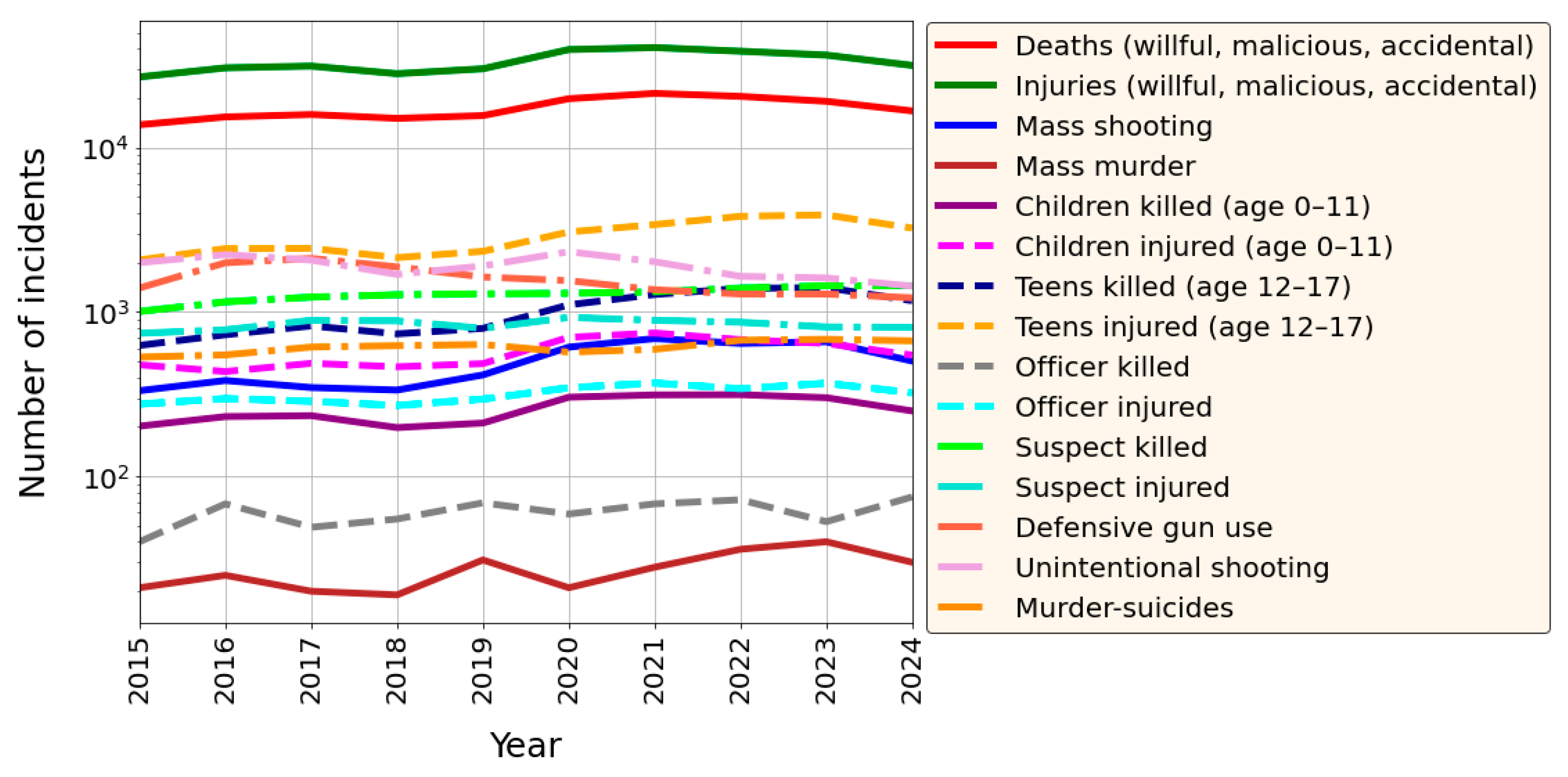
Figure 1. Number of gun incidents in the U.S. in the last decade [1].
Electronics 14 03540 g001
Figure 2. The processes flow of the research performed.
Electronics 14 03540 g002
Figure 3. Examples of transformations performed during augmentation of a self-prepared dataset: (a) affine transformations; (b) safe rotate; (c) shift scale rotate; (d) perspective; (e) random brightness; (f) Gaussian blur.
Electronics 14 03540 g003
Figure 4. Categories of images included in the second part of the dataset: (a) items clearly visible; (b) items partially covered; (c) small items; (d) poor image sharpness; (e) poor image illumination; (f) sample background images.
Electronics 14 03540 g004
Figure 5. The structure of the datasets used. The pie charts provide information on the number of items belonging to a specific class.
Electronics 14 03540 g005
Figure 6. The YOLO model architecture [31].
Electronics 14 03540 g006
Figure 7. Illustration of the IoU parameter for the predicted box Bp (green) and the ground-truth box Bgt (blue).
Electronics 14 03540 g007
Figure 8. Plots of training and validation losses (a) and plots of basic detection quality metrics for the validation set (b) built for the YOLOv11m model.
Electronics 14 03540 g008
Figure 9. Models’ recall and inference time.
Electronics 14 03540 g009
Figure 10. Evaluation results of the models selected in Figure 9.
Electronics 14 03540 g010
Figure 11. Models’ mAP@50–95 and complexity (number of parameters).
Electronics 14 03540 g011
Figure 12. Recall of detection of individual items by models selected from Figure 11.
Electronics 14 03540 g012
Figure 13. Models’ inference time and complexity (number of parameters).
Electronics 14 03540 g013
Figure 14. YOLOv11m model confusion matrix built for the test set.
Electronics 14 03540 g014
Figure 15. Examples of prediction results of images from the test set performed by the YOLOv11m model: (a) small items; (b) poor image sharpness; (c) poor image illumination.
Electronics 14 03540 g015aElectronics 14 03540 g015b
Figure 16. Example results of prediction of images captured by surveillance camera performed by YOLOv11m model: (a) items clearly visible; (b) small items; (c) poor image sharpness; (d) poor image illumination.
Electronics 14 03540 g016
Figure 17. General structure of the system implementing the YOLOv11m model.
Electronics 14 03540 g017
Table 1. Publicly available image datasets used to detect dangerous items.
Dataset Name (Source)No. of Images (Classes)Refs.
Pistols Dataset (Roboflow)2986 (guns)[14]
OD-WeaponDetection (GitHub)5859 (guns, knives, backgrounds)[15]
Weapon Detection Dataset (Kaggle)714 (various weapons)[16]
Gun Detection Datasets (LinkSprite)51,000 (guns)[17]
Pistols-YoloV5 Object Detection Dataset (Roboflow)6752 (guns)[18]
Pistol Labeled Image Dataset (Images.CV)7400 (guns)[19]
Weapons Labeled Image Dataset (Images.CV)40,000 (various weapons)[20]
Weapons in Images (Dataset Ninja)5695 (various weapons)[21]
Weapon detection dataset (Kaggle)3000 (guns)[22]
Weapon detection system (GitHub)4940 (guns)[23]
Mock Attack Dataset (GitHub)5149 (knives, rifles)[24]
Gun and Knife Detection (Roboflow)8451 (guns, knives)[25]
Pistol and Rifle and Knife Dataset (Roboflow)12,932 (guns, knives, rifles)[26]
Gun and Knife Detection System Dataset (Roboflow)2402 (guns, knives)[27]
YouTube-GDD (GitHub)5000 (guns, rifles)[28]
Weapons-Dataset (GitHub)7801 (guns, rifles)[29]
Table 2. Specification of transformations performed during augmentation of a self-prepared dataset.
Type of Transf.Albumentations FunctionParameterValue/Range
Spatial-level
transforms
Affinerotate45
scale[0.5, 2]
shear15
translate_percent0.05
SafeRotatelimit90
ShiftScaleRotateshift_limit0.0625
scale_limit0.1
rotate_limit45
Perspectivescale[0.15, 0.2]
Pixel-level
transforms
RandomBrightnessContrastbrightness_limit[−0.2, −0.1]
contrast_limit[0, 0]
GaussianBlursigma_limit[3, 5]
Table 3. Selected hyperparameters used during the models training and validation process.
NameValue
epochs—total number of training epochs200
patience—number of epochs to wait without improvement in validation metrics before early stopping the training100
batch—batch size32
imgsz—target image size for training640
optimizer—choice of optimizer for trainingSGD
momentum—momentum factor influencing the incorporation of past gradients in the current update0.937
lr0—initial learning rate0.01
lrf—final learning rate as a fraction of the initial rate = (lr0 × lrf), used in conjunction with schedulers to adjust the learning rate over time0.01
weight_decay—L2 regularization term, penalizing large weights to prevent overfitting0.0005
warmup_epochs—number of epochs for learning rate warmup, gradually increasing the learning rate from a low value to the initial learning rate to stabilize training early on3.0
warmup_momentum—initial momentum for warmup phase, gradually adjusting to the set momentum over the warmup period0.8
warmup_bias_lr—learning rate for bias parameters during the warmup phase, helping stabilize model training in the initial epochs0.1
box—weight of the box loss component in the loss function, influencing how much emphasis is placed on accurately predicting bounding box coordinates7.5
cls—weight of the classification loss in the total loss function, affecting the importance of correct class prediction relative to other components0.5
dfl—weight of the distribution focal loss, used in certain YOLO versions for fine-grained classification1.5
iou—sets the Intersection Over Union threshold for Non-Maximum Suppression0.7
max_det—limits the maximum number of detections per image300
augment—enables test-time augmentation during validationfalse
Table 4. Models’ evaluation results.
ArchitectureVersionPrecisionRecallmAP@50mAP@50–95
YOLOv8n0.8880.8420.8970.670
s0.9100.8430.9040.709
m0.9090.8690.9110.736
l0.9090.8650.9120.741
x0.9330.8690.9230.752
YOLOv9t0.8870.8500.8990.691
s0.9140.8730.9090.728
m0.9120.8810.9090.740
c0.9300.8520.9150.740
e0.9160.8720.9170.750
YOLOv10n0.8680.8370.8880.672
s0.9220.8370.9020.709
m0.9240.8440.9030.727
l0.9350.8620.9150.742
x0.9210.8360.9120.739
YOLOv11n0.8970.8300.8900.666
s0.9030.8430.9050.713
m0.8960.8820.9180.737
l0.9140.8700.9160.741
x0.9270.8590.9160.743
YOLOv12n0.9010.8160.8900.681
s0.8870.8710.9120.719
m0.9060.8660.9160.733
l0.9210.8750.9200.738
x0.9180.8690.9180.746
RT-DETRl0.9270.8850.8990.698
x0.9280.8890.8950.710
Table 5. Results of research on the detection of dangerous items. A standard IoU threshold of 0.50 was used for all measures.
Refs.Network/
Backbone
mAP (%)Precision (%)Recall (%)
Own resultsYOLOv11m/C3K291.8 (baseball bat,
gun, knife,
machete, rifle)
88.3 (machete)
84.4 (knife)
89.6 (baseball bat)
95.1 (rifle)
90.5 (gun)
81.1 (machete)
84 (knife)
93.8 (baseball bat)
93.1 (rifle)
88.8 (gun)
[55]YOLOv8/CSPDarknet-5378 (weapon, no weapon)85 (weapon)80 (weapon)
[56]YOLOv3/Darknet-5398.9 (10 weapon classes)
[54]YOLOv8/CSPDarknet-5357.2 (knife)
[50]YOLOv5s/CSPDarknet-5381 (gun)99 (gun)
[53]YOLOv5/CSPDarknet-5395 (gun)98 (gun)87 (gun)
[57]YOLOv3/Darknet-5380 (gun)74 (gun)
[58]YOLOv4/CSPDarknet-5391.7 (gun)93 (gun)88 (gun)
[51]FMR-CNN + YOLOv8/MobileNetV3 + CSPDarknet-5390.1 * (pistol, revolver, rifle, hand-held firearms, gun)97.2 (pistol, revolver, rifle, hand-held firearms, gun)95 (pistol, revolver, rifle, hand-held firearms, gun)
[52]YOLOv7-DarkVision/Extended-ELAN95.7 (gun)95.5 (gun)91.4 (gun)
[13]Faster R-CNN/ResNet15285
(baseball bat,
gun, knife,
machete, rifle)
87.8 (baseball bat)
91.3 (gun)
80.8 (knife)
79.7 (machete)
85.3 (rifle)
95.3 (baseball bat)
94.6 (gun)
90 (knife)
85.5 (machete)
88.5 (rifle)
[59]Faster R-CNN/CNN84.7 (gun)86.9 (gun)
[60]Faster R-CNN/CNN84.6 (gun, rifle)
[61]Faster R-CNN/VGG-1684.2 (gun)100 (gun)
[62]Faster R-CNN/ResNet5080.5
(axe, gun, knife,
rifle, sword)
96.6 (gun)
55.8 (knife)
100 (rifle)
61 (gun)
52 (knife)
96 (rifle)
[63]Faster R-CNN/VGG-1679.8
(gun, rifle)
80.2 (gun)
79.4 (rifle)
[64]Faster R-CNN/Inception-ResNetV279.3 (gun)68.6 (gun)
[65]Faster R-CNN/ResNet5088.1 (gun)100 (gun)
[58]Faster R-CNN/Inception-ResNetV286.4 (gun)89.2 (gun)
[66]Faster R-CNN/SqueezeNet85.4 (gun)
Faster R-CNN/GoogleNet46.7 (knife)
* mAP@50–95.
Disclaimer/Publisher’s Note: The statements, opinions and data contained in all publications are solely those of the individual author(s) and contributor(s) and not of MDPI and/or the editor(s). MDPI and/or the editor(s) disclaim responsibility for any injury to people or property resulting from any ideas, methods, instructions or products referred to in the content.