Network Splitting Techniques and Their Optimization for Lightweight Ternary Neural Networks

Abstract

To run a high-performing deep convolutional neural network (CNN), substantial memory and computational resources are typically required. To address this, we propose an optimization method of a ternary neural network (TNN) by applying network splitting techniques to achieve an even more lightweight model. TNN offers a favorable trade-off between accuracy and computational saving compared to a binary quantized network, which often suffers from higher accuracy loss due to extreme quantization. Our network splitting technique combines grouped convolution and pointwise convolution, where the convolution operations are computed in separate groups and then the features are fused together in the later step. Our proposed network splitting technique has the advantage of being easily implemented with lightweight hardware design. For example, when implementing Processing-In-Memory (PIM) hardware, each convolution layer can be set to the same size, enabling the design of lightweight neural network accelerators by eliminating the need for analog-to-digital conversion. As a result, our experiments show that the proposed method can save up to 4.53× memory compression with minimal impact on the accuracy.

1. Introduction

In recent years, artificial intelligence (AI) has been integrated into daily life, with applications including virtual assistants, photo and video enhancement, and various text and speech processing tasks. Deep convolutional neural network (CNN) plays a crucial role in the growth of AI technologies. However, high-performance CNNs typically demand high memory and computational resources, making it difficult for them to be implemented on mobile devices. To address this issue, research on efficient neural networks has gained significant attention within the machine learning domain. One of the most popular approaches is to reduce the floating-point precision into lower bit representations, thereby compressing both storage requirements and computational complexity.

Network quantization is a popular technique to reduce the full precision parameters into a low bit format. BMNN [1,2] binarizes Multilayer Neural Networks with Expectation BackPropagation (EBP). BinaryConnect [3] implements a highly quantized network by constraining the weights’ value to +1 and −1, and extends it to activation in Binarized Neural Network (BNN) [4]. XNOR-Net [5] introduces binarized weight and input with scaling factors and utilizes XNOR and bitcount operation for convolution operations. DoReFa-Net [6] develops bitwidth gradients in backward propagation. ABC-Net [7] introduces multiple binary weight bases and binary activations. Despite the positive impact of binarized networks on efficiency, they often suffer from a notable accuracy degradation. Hence, the use of ternary states has been explored further in ternary neural networks (TNNs) due to their significantly more accurate results compared to the binary states of BNNs. A TWN [8] ternarizes only the weight while maintaining full-precision inputs, resulting in high accuracy but less memory saving. Other researchers [9,10,11] utilize a pre-trained full-precision model as initial weight prior to ternarization. The TNN proposed in [12] uses the teacher–student method for training, in which the teacher network uses full-precision weight parameters. TRQ [13] combines a binarized stem and residual parts to enhance the quantization thresholding. Furthermore, a combination of ternary and binary networks was also introduced in TBN [14] to balance efficiency and classification accuracy.

While neural network quantization methods have demonstrated improvements in energy efficiency, often, techniques to reduce complexity and power consumption do not consider compatibility with the hardware system. To bridge this gap, several studies have proposed hardware designs to cater for these neural network enhancements. For instance, FATNN [15] modifies bit operations in TNN to improve hardware compatibility. xTern [16] optimizes kernels using an extension of RISC-V instruction set architecture for TNN inference. ISAAC [17], PRIME [18], and Eyeriss [19] are accelerators developed specifically for CNNs. T-CIM [20] proposes a ternary bitcell architecture particularly designed for a TNN accelerator. Additionally, a scalable RRAM-based BNN accelerator [21] is proposed with network reconstruction and retraining.

The developments of those hardware systems highlight the need for hardware-aware neural network design to optimize the performance and efficiency of both aspects. Rather than separately addressing neural network optimization and hardware acceleration, adopting a co-design between the two could maximize the joint benefits. This is particularly important for implementation on edge devices with limited computational resources. To address this, we introduce a network splitting technique such that the split partitions represent each hardware array. By matching the number of operations to the corresponding array, each convolution could be performed in each array, thereby eliminating the conversion from analog to digital. Moreover, this method is scalable and can be integrated into various neural network architectures, aiming to reduce computational overhead while maintaining high inference accuracy.

This paper makes the following key contributions:

• We propose a co-design approach between neural network and hardware to achieve more efficient computation energy usage. The convolutional operations in the neural network are split into groups, where each group fits the hardware array for computation so that the output activation operations are performed in each array. Thus, the analog-to-digital converter (ADC) can be entirely removed from the PIM hardware design. In addition, this method is applicable to various architectures, including a large-scale neural network.
• We evaluate the proposed network splitting technique in TNN and compare its performance with XNOR-Net, a widely used BNN. Our experiments on CIFAR-10 and CIFAR-100 datasets show that the proposed scheme can maintain comparable inference accuracy to the original network, even in a large architecture such as ResNet-20. The proposed design offers a trade-off between memory, computational saving, and accuracy, achieving significant savings with minimal performance degradation.

The rest of the paper is organized as follows. In Section 2, we cover the related preliminary works, including network quantization, residual network architecture, and grouped and pointwise convolution. Section 3 contains the details of our proposed network splitting technique and TNN algorithm. Section 4 presents the experimental setup, results, and a discussion of our method on CIFAR-10 and CIFAR-100 datasets. Finally, Section 5 concludes the paper.

2. Preliminary Works

2.1. Network Quantization

2.1.1. Ternary Neural Network

Ternary neural network (TNN) offers a trade-off between classification performance and computational saving by constraining the value of both weight and input to {−1, 0, +1}. In this paper, we follow the method from TWN [8] to estimate the ternary weight, and we extend the implementation for input ternarization. During forward propagation, we utilize symmetric threshold [22] to determine the ternarization value, where in each layer $l$, the threshold for weight $w$, ${∆}_w^l$, and the threshold for input $x$, ${∆}_x^l$, are described below.

$${∆}_w^l=\delta \times max\left({\left|w\right|}_l\right),$$

(1)

$${∆}_x^l=\delta \times max\left({\left|x\right|}_l\right),$$

(2)

where $\delta$ denotes a constant representing thresholding factor. The value of the threshold is particularly important, as it affects the distribution of ternarized weights and activations. When the threshold is equals to 0, the ternarized output will be just −1 and +1, which makes it binarized instead.

After obtaining the threshold, we define the scaling factor for weight ($\mathsf{\alpha }$) and input ($\beta$) as follows

$$\mathsf{\alpha }={\displaystyle \frac{1}{n}}\left|w_l\right|,$$

(3)

$$\beta ={\displaystyle \frac{1}{n}}\left|x_l\right|,$$

(4)

where $n$ is the number of weight or input in layer $l$. Essentially, the scaling factor is the mean of absolute value for each weight and input in the selected layer. Only weights and inputs that are greater than their respective thresholds are calculated. Finally, the ternarized weight ($w_t$) and input ($x_t$) are formulated below.

$$w_t=\left\{\begin{array}{c}-\alpha , w\le -∆\\ 0, \left|w\right|<∆\\ \alpha , w\ge ∆ \end{array}\right.,$$

(5)

$$x_t=\left\{\begin{array}{c}-\beta , x\le -∆\\ 0, \left|x\right|<∆\\ \beta , x\ge ∆ \end{array}\right.,$$

(6)

With the above ternary weights and inputs, the dot product can be expressed as below.

$$w_t{·x}_t=\left(\alpha ·Tern\left(w\right)\right)·\left(\beta ·Tern\left(x\right)\right)=\alpha \beta ·\left(Tern\left(w\right)·Tern\left(x\right)\right),$$

(7)

where $Tern\left(w\right)$ and $Tern\left(x\right)$ are the ternarized value of weight and input, respectively, limited to the value of −1, 0, and +1. Therefore, the operation can be calculated by simply using addition and subtraction, avoiding the computational overhead of floating-point multiplication.

However, the full-precision values of weights are retained for parameter updates in the backward propagation. We use Straight-Through Estimator (STE) [23] to calculate the gradient during back-propagation, since the derivative of the ternarization function is zero almost everywhere. The gradients can be described in the equation below.

$${\displaystyle \frac{\partial g}{\partial w}}=\left\{\begin{array}{c}{\displaystyle \frac{\partial g}{\partial w_t}}, \left|w\right|\le 1\\ 0,\hspace{1em}\hspace{1em} otherwise\end{array}\right.,$$

(8)

where the gradients are calculated with respect to ternarized weight ($w_t$) if the real-valued weight is within threshold, and otherwise clipped to prevent explosion. Then, the full-precision parameter values are updated before going to the next iteration.

2.1.2. XNOR-Net

XNOR-Net [5] is a binary neural network implementation which limits the input and weight into binary values with the use of scaling factor. The binary value of weight $w$ and input $x$ can be expressed with the following equations.

$$w_b=\alpha ·sign\left(w\right),$$

(9)

$$x_b=\beta ·sign\left(x\right),$$

(10)

where $w_b$ and $x_b$ are the binarized weight and input, respectively. $\alpha$ and $\beta$ represent the scaling factor of weight and input, described as the average of the absolute value of the original full-precision weights and inputs. As the weight and input are binary, the convolution operation can be approximated by XNOR and bitcount operation, as formulated below.

$$w_b \ast x_b\approx \alpha \beta ·\left(sign\left(w\right) \ast sign\left(x\right)\right),$$

(11)

where the convolution between $sign\left(w\right)$ and $sign\left(x\right)$ can be simplified using XNOR and bitcount operations. As with TNN, the binarized values are used for gradients computation during back-propagation, while the parameter update is calculated on the full-precision values.

2.2. Residual Network

Residual network (ResNet) [24] proposes a skip connection, also known as shortcut, in deep neural networks. This implementation aims to prevent the degradation problem, where deeper networks are prone to a higher training error due to the saturation of training data. In deeper layers, the gradients of the loss function often vanish (approach zero) or explode (grow too large), making training unstable. To address this issue, ResNet introduces residual learning and identity mapping as the main idea in the proposed method, where a ResNet architecture is formed by stacking these residual blocks together.

Figure 1 shows the basic building block of residual learning. The input from the previous layer is processed in two paths. The first path consists of a set of convolution layers with intermediate ReLU [25] activation function. The second path is the skip connection, which directly passes the input forward. If the input and output are of the same size, identity mapping is applied; otherwise, a 1 × 1 convolution is performed to align the dimension. The outputs of both paths are then integrated using element-wise addition, and the combined result is passed through ReLU activation to produce the final output of the residual block. It is worth noting that the shortcut does not require additional parameters and computation, making it an effective architectural enhancement.

2.3. Grouped Convolution

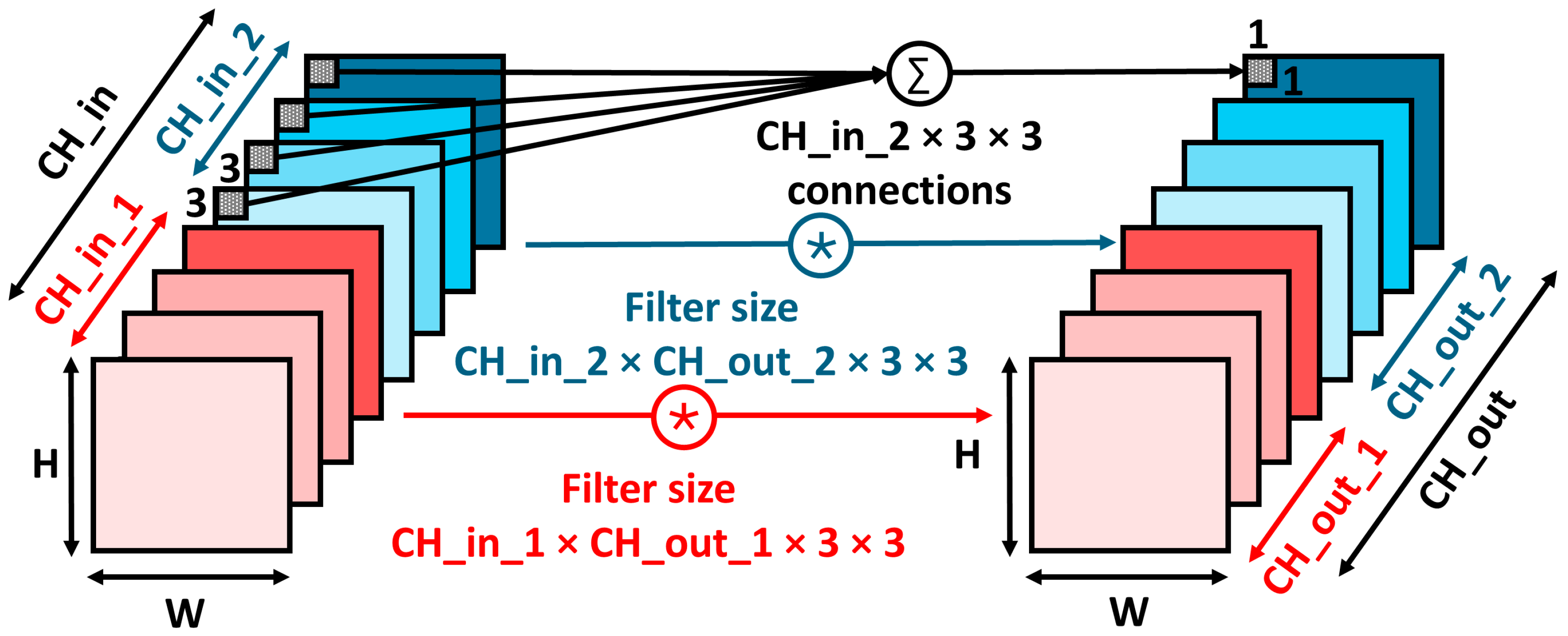
Grouped convolution was introduced in AlexNet [26], where it was utilized for parallel processing. This technique involves dividing the input channels into multiple groups and performing convolution independently, resulting in a lower number of parameters and less computational complexity. Figure 2 illustrates an example of a grouped convolution with two groups. CH_in represents the number of channels in the input feature map, which are split into two groups, CH_in_1and CH_in_2, such that the length of each group is half of the original channel. Each group’s convolutions are handled with a separate set of weight filters, which leads to separate output channels, CH_out and CH_out_2. The sum of connections to produce an output feature map is equal to the weight kernel size multiplied by the number of input channels. Thus, in Figure 2, one feature map in CH_out_2 can be calculated as 3$\times$ 3 $\times$ CH_in_2, where CH_in_2 denotes the number of input channels in the group.

2.4. Pointwise Convolution

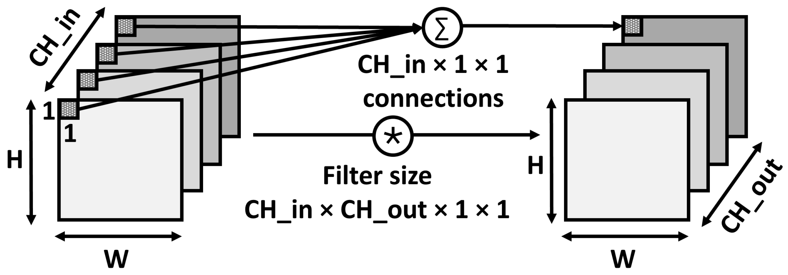
Pointwise convolution is a convolution operation that uses a $1\times 1$ weight kernel. A similar approach was used in the MLP convolution layer of NIN [27]. This type of convolution is commonly used to change the dimensionality or number of channels of the input. Additionally, it can be used to combine channels from different grouped outputs, fusing their features. Thus, information sharing across groups can be obtained on this stage. Figure 3 shows the illustration of the operation in a pointwise convolution. Convolutions are performed on each $1\times 1$ input feature of every channel, producing one result in the output channel. As a result, the height (H) and width (W) of the input are preserved in the output feature map.

3. Proposed Method

3.1. Network Splitting Technique

We propose a network splitting technique as shown in Figure 4. Figure 4a shows the original convolution operation in standard CNN, where a $3 \times 3$ weight kernel is used. The filter size for one convolution layer is equal to the multiplication of the number of input channels (CH_in), the number of output channels (CH_out), and kernel size ($3 \times 3$). To produce one output pixel, CH_in $\times$ 3 $\times$ 3 connections are required, which represents one set of multiply–accumulate (MAC) operations. Figure 4b shows the proposed split network, where the input channels are divided into groups according to the hardware design, such that one group represents each PIM hardware array. The advantage of the network splitting technique is that MAC operations can be performed in small PIM hardware arrays without analog-to-digital conversion by performing the activation directly from the small PIM arrays. On the other hand, when the network is not split, a power-hungry ADC is required since MAC results calculated in several small PIM arrays should be converted into multi-bit data to obtain the input of the activation function by adding each multi-bit MAC result.

The proposed method consists of two main steps. The first step is to split the convolutional layer using grouped convolution. The number of connections within one group should not surpass the array size of the PIM hardware. For instance, if there are 32 input channels and a hardware array size of 144, the convolution should be grouped into 2, where each group has $16 \times 3 \times 3$ connections to produce one output. Thus, the number of connections in this grouped convolution can fit into the hardware array to obtain output activation results directly. The input channel, output channel, and filter size are separated into two and convoluted independently, according to their respective groups.

However, grouped convolution prevents gradients from flowing across different groups, thereby resulting in a performance drop. To recover the loss of accuracy from the split, an additional convolution layer is added as the second step. We use a pointwise convolution layer in step two, where the channel mixing feature helps to share information across multiple groups. Each $1\times 1$ input feature from all groups is convoluted with a $1\times 1$ kernel of the pointwise layer and produces one output feature map. This step ensures that the features from different groups are fused in the output channel. However, if there is no grouping in the previous step, pointwise convolution is not necessary; therefore, an identity operator can be used as a replacement. Algorithm 1 shows the splitting technique details in pseudo-code.

Algorithm 1: Network splitting technique on a convolution operation

Input: Hardware array size ($dim$), input channel size ($in\_planes$), output channel size ($planes$) 1: $conn\leftarrow in\_planes\times 3\times 3$ // number of connections to produce one output 2: $groups\leftarrow \left(conn+dim-1\right)/dim$ // calculate number of groups 3: $conv1\leftarrow Conv2d(in\_planes,planes,kernel\_size=3,stride=1,padding=1,groups=groups)$ // grouped convolution 4: if $groups=1$ then // no grouping, continue with identity 5:  $conv2\leftarrow Identity$ 6: else // pointwise convolution to share information across groups 7: $conv2\leftarrow Conv2d(planes,planes,kernel\_size=1,stride=1,padding=0)$

3.2. TNN Training

The training process follows the TNN framework as described in Section 2.1.1. Algorithm 2 details the TNN training method in each iteration. First, in each layer, the full-precision weights and inputs are converted into their respective ternarized values. The steps are as described in Equations (1)–(6), where the threshold is defined as the maximum absolute value of the weight or input in the layer, with consideration of the thresholding factor. Next, we identify the scaling factor, which is the average of the absolute value of weights or inputs. For each weight and input, the ternarized values are calculated based on the corresponding threshold.

After obtaining the ternary value of the weights and inputs, forward propagation is performed using those values. It should be noted that the convolution layers implement the network splitting technique from Section 3.1. Then, the gradients are calculated in the backward propagation with respect to the ternary weight, while the parameter updates are performed on the full-precision weight. Finally, the learning rate is adjusted using any chosen scheduling function.

Algorithm 2: Neural network training with ternarized weight and input

Input: Batch of input and target output ($x,y$), cost function $C(y,y^{\prime })$, full-precision weight ($w$), learning rate ($\eta$), thresholding factor ($\delta$) Output: updated weight and learning rate 1: for $l\leftarrow 1$ to $L$ do 2: ${∆}_w^l\leftarrow \delta \times max\left({\left|w\right|}_l\right)$ // find threshold for weight ternarization in this layer 3: $\alpha \leftarrow {\displaystyle \frac{1}{n}}\left|w_l\right|$ 4: for $w$ in $l$ do // ternarize weight 5:   $w_t\leftarrow \alpha ·Tern\left(w,{∆}_w^l\right)$ 6: ${∆}_x^l\leftarrow \delta \times max\left({\left|x\right|}_l\right)$ // find threshold for input ternarization in this layer 7: $\beta \leftarrow {\displaystyle \frac{1}{n}}\left|x_l\right|$ 8: for $x$ in $l$ do // ternarize input 9:   $x_t\leftarrow \beta ·Tern\left(x,{∆}_x^l\right)$ 10: $y^{\prime }\leftarrow forward(w_t,x_t)$ // forward propagation with convolution using network splitting technique and ternarized weight and input 11: ${\displaystyle \frac{\partial C}{\partial w_t}}\leftarrow backward({\displaystyle \frac{\partial C}{\partial y^{\prime }}}, w_t)$ // backward propagation using ternary weight 12: $w\leftarrow update\_parameter(w,{\displaystyle \frac{\partial C}{\partial w_t}},\eta )$ // parameter update using real-valued weight 13: $\eta \leftarrow update\_learning\_rate\left(\eta \right)$

4. Experimental Results

4.1. Experimental Setup

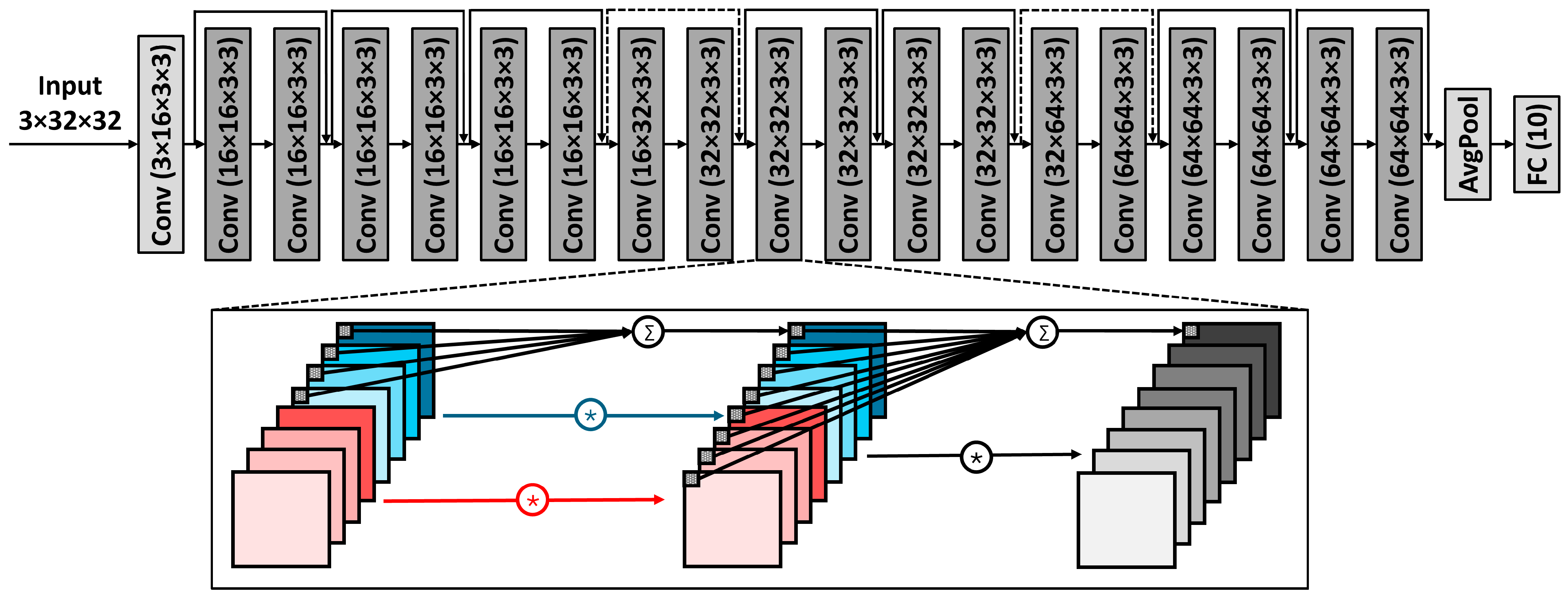
To evaluate the performance of the proposed method, we use the image classification datasets CIFAR-10 and CIFAR-100 [28], each of which consists of 50,000 training data and 10,000 test data. The datasets are composed of $32\times 32$ color images, divided into 10 and 100 classes for CIFAR-10 and CIFAR-100, respectively. We implement TNN with the proposed network splitting technique on ResNet-20 architecture and compare the results with a modified version of XNOR-Net [5], with the same splitting method and network architecture. The ternarization and network splitting are limited on the residual blocks, while the first convolutional layer and the fully connected layer are using full-precision weights and inputs. Figure 5 shows the illustration of ResNet-20 architecture used in our experiments. Each residual block consists of two convolutional layers, with a channel size of 16, 32, and 64 across different stages. There are three residual blocks per stage, resulting in a total of 18 intermediate convolutional layers throughout the network.

We conducted experiments with different settings of split size configurations. As a baseline, we first evaluated the network without any splitting. Next, we split the 144 connections (corresponding to 16 channels) into two groups, while leaving the remaining layers unsplit. Subsequently, we extended the split mechanism to all the convolution layers with configurations of 144, 72, and 36 connections per group. The complete configurations are listed in

Table 1. Split size configurations with the corresponding number of groups and connections for each input channel.

Configurations	Number of Groups × Connections
	16 Channels	32 Channels	64 Channels
No Split	1 × 144	1 × 288	1 × 576
144 → 2 × 72	2 × 72	1 × 288	1 × 576
All split to 144	1 × 144	2 × 144	4 × 144
All split to 72	2 × 72	4 × 72	8 × 72
All split to 36	4 × 36	8 × 36	16 × 36

. The parameters used for each configuration are optimized independently. The range of parameters is provided in

Table 2. Parameters used in the experiment.

Parameter	Value
Number of epochs	3000
Batch size	128
Learning rate	0.06–0.3
Weight decay	4 × 10−6–9 × 10−4
Thresholding factor	0.02–0.04

. All experiments were trained using the stochastic gradient descent (SGD) optimizer with a cosine annealing learning rate scheduler.

4.2. Results and Discussion

The experimental results are summarized in

Table 3. Experiment results of TNN and XNOR-Net for the CIFAR-10 dataset, with various split size configurations, with accuracy drop compared to no split.

Split Size Configuration	TNN (This Work)		XNOR-Net [5]
	Accuracy (%)	Drop (%)	Accuracy (%)	Drop (%)
No Split	88.38 (±0.20)	-	83.23 (±0.05)	-
144 → 2 × 72	87.14 (±0.12)	1.24	82.68 (±0.07)	0.55
All split to 144	86.18 (±0.05)	2.20	76.16 (±0.52)	7.07
All split to 72	83.51 (±0.09)	4.87	70.43 (±2.51)	12.80
All split to 36	80.97 (±0.50)	7.41	67.73 (±2.31)	15.50

and

Table 4. Top-1/top-5 results of TNN and XNOR-Net for the CIFAR-100 dataset, with various split size configurations, with accuracy drop compared to no split.

Split Size Configuration	TNN (This Work)			XNOR-Net [5]
	Top-1 (%)	Top-5 (%)	Drop (%)	Top-1 (%)	Top-5 (%)	Drop (%)
No Split	61.33 (±0.28)	87.10 (±0.29)	-	53.56 (±0.06)	81.58 (±0.14)	-
144 → 2 × 72	59.35 (±0.15)	86.00 (±0.23)	1.98/1.10	53.25 (±0.27)	81.25 (±0.22)	0.31/0.33
All split to 144	53.98 (±0.91)	82.60 (±0.73)	7.35/4.50	44.01 (±0.13)	74.25 (±0.13)	9.55/7.33
All split to 72	49.64 (±1.09)	79.46 (±0.99)	11.69/7.64	34.79 (±1.41)	64.71 (±1.39)	18.77/16.87
All split to 36	48.09 (±0.39)	78.36 (±0.16)	13.24/8.74	32.17 (±3.49)	62.68 (±3.55)	21.39/18.9

. We examine and compare the impact of the proposed network splitting technique on quantized networks (TNN and XNOR-Net). Without any splitting, TNN achieves an accuracy of 88.38% in the CIFAR-10 dataset using the ResNet-20 architecture, outperforming XNOR-Net by 5.15%. Upon splitting the 144 connections (corresponding to 16 channels) into two groups of 72, TNN experiences a 1.24% accuracy reduction, while XNOR-Net shows a smaller reduction of 0.55%. In the subsequent experiments where all convolutional layers in the residual blocks are split, TNN displays a gradually decline in accuracy by approximately 2% in each level, with 2.20%, 4.87%, and 7.41% accuracy loss when the connections are split into groups of 144, 72, and 36, respectively, compared to the original TNN. Meanwhile, XNOR-Net suffers from a significant drop when all the layers are split. When all connections are split to 144, there is a 7.07% drop compared to the baseline. Furthermore, splitting into groups of 36 connections reduces the accuracy sharply to 67.73%, a 15.50% decrease from the accuracy of no split. These findings suggest that TNN exhibits greater robustness to network splitting, maintaining relatively stable performance across configurations. On the other hand, XNOR-Net is unable to capture the interactions of features across different groups, leading to the substantial degradation in classification accuracy.

The results for the CIFAR-100 dataset show a similar trend, where splitting 144 connections into 72 reduces the accuracy of XNOR-Net by less than 1%. For both networks, the decline in accuracy is more significant in top-1 accuracy than in top-5 accuracy. When all the convolutional layers are split, TNN shows a smaller accuracy drop compared to XNOR-Net. Moreover, the results of TNN remain relatively consistent with small standard deviation on the classification accuracy result, while XNOR-Net shows larger fluctuations with up to 3.55% standard deviation in the top-5 result.

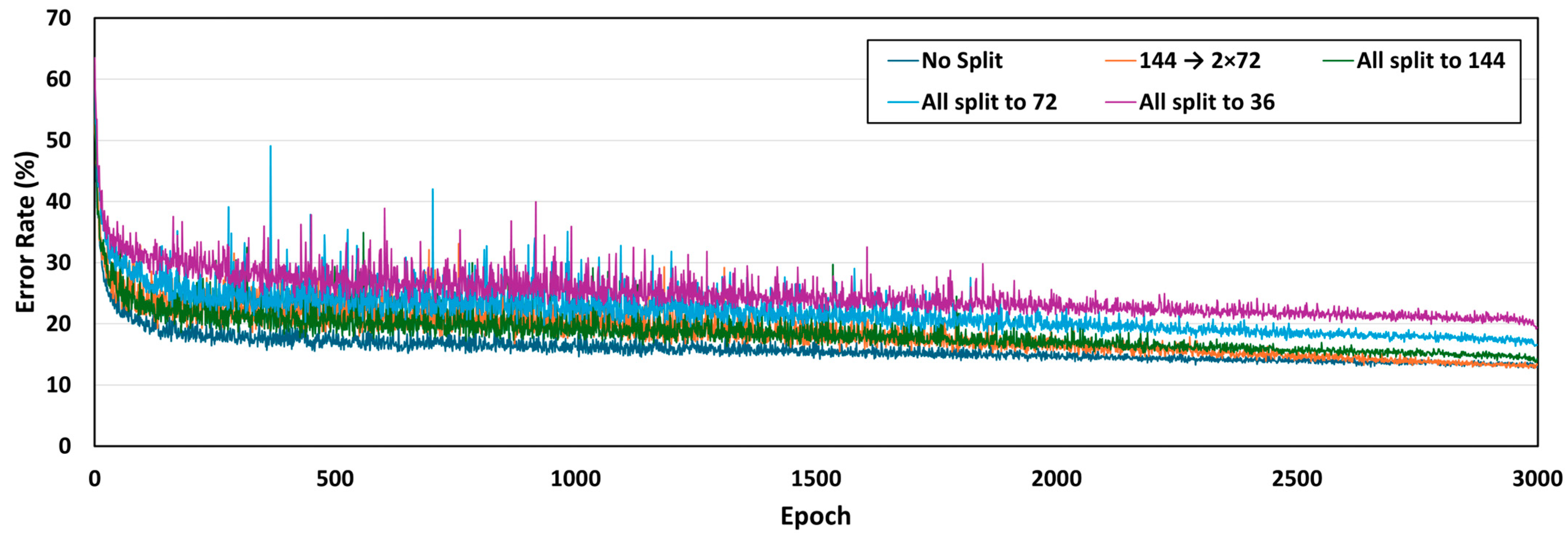
Figure 6 illustrates the evolution of the error rate in the training process. In the early epochs, all split configurations exhibit notable fluctuations. As the training progresses, the split configurations with a larger number of connections stabilize more quickly and converge into better accuracy. In contrast, the configuration with fewer connections continues to fluctuate and is unable to achieve comparable performance.

Next, we examined the number of parameters to estimate the memory saving of the split network in TNN. Due to the grouping, the input channels only connected to its corresponding group of output channels. This leads to fewer connections and hence a smaller number of weight parameters is required for the convolution operations.

Table 5. Number of parameters and the respective memory saving in TNN split networks.

Split Configuration	Number of Parameters	Memory Saving
No Split	270,538	1.00×
144 → 2 × 72	263,882	1.02×
All split to 144	129,738	2.08×
All split to 72	83,914	3.22×
All split to 36	59,722	4.53×

shows the number of parameters and the estimated memory saving for each of the split configurations. Compared to no split as a baseline, splitting 144 connections into two groups of 72 only saves 1.02× memory, due to the fact that only seven convolutional layers are grouped. However, when all the convolutional layers within the residual blocks are split, they acquire more substantial memory savings with 2.08×, 3.22×, and up to 4.53× for 144, 72, and 36 connections per group, respectively. Furthermore, the reduction in connections in the convolution operation lessens the computation required to produce output features, thus contributing to improved efficiency. In addition to evaluating split network accuracy and saving, we investigated the effect of the thresholding factor in TNN to determine the optimal value for ternarization. When the thresholding factor is equal to zero, the ternary outputs are limited to −1 and +1, making it similar to binarization. On the other hand, when the thresholding factor is too large, there will be too many zeroes as ternary output, causing a degradation to the model’s performance due to information loss. Figure 7 illustrates the impact of various thresholding factors on classification accuracy. The graph shows that the accuracy reaches its peak when the thresholding factor is in the range of 0.02-0.04 and declines afterwards. For the configurations of no split, all split to 72, and all split to 36, the optimal accuracy is achieved at 0.03. Meanwhile, the best results for split 144 → 2 × 72 and all split to 144 are observed at 0.02 and 0.04, respectively.

Overall, our proposed network splitting technique in TNN demonstrates more robust performance compared to XNOR-Net, especially when the number of connections per group is reduced. When all the convolutional operations in the residual blocks are split, the smaller number of connections in a group creates more fluctuation during training, resulting in a higher accuracy loss but increased memory saving. When all connections are split to 144, a slight accuracy reduction of 1.24% in CIFFAR-10 and 1.10% in CIFAR-100 (top-5) is observed compared to the original network, while achieving a 2.08× memory saving. In contrast, splitting into 36 connections provides up to 4.53× memory saving, with an accuracy loss of 7.41% in CIFAR-10 and 8.74% in CIFAR-100 (top-5). Additionally, in TNN training, the thresholding factor is an important aspect to optimize, where the optimal thresholding factor value across all configurations is consistently observed in the range of 0.02–0.04.

5. Conclusions

In this work, we propose a novel network splitting technique for lightweight ternary neural networks (TNNs). The splitting technique is implemented such that each group contains a matching number of operations with the PIM hardware array, thereby eliminating the need of analog-to-digital conversion. The proposed method consists of grouped convolutions to perform convolution operations independently, and pointwise convolutions to fuse the features of the separated channels. The experimental results of the network splitting implementation on TNN reflect a robust and stable performance across various split configurations, achieving notable memory and computational savings with minimal accuracy loss.

References

1. Cheng, Z.; Soudry, D.; Mao, Z.; Lan, Z. Training Binary Multilayer Neural Networks for Image Classification Using Expectation Backpropagation. arXiv 2015, arXiv:1503.03562. [Google Scholar] [CrossRef]
2. Soudry, D.; Hubara, I.; Meir, R. Expectation Backpropagation: Parameter-Free Training of Multilayer Neural Networks with Continuous or Discrete Weights. In Proceedings of the Advances in Neural Information Processing Systems 2 Conference: Neural Information Processing, Montreal, QC, Canada, 8 December 2014. [Google Scholar]
3. Courbariaux, M.; Bengio, Y.; David, J.-P. BinaryConnect: Training Deep Neural Networks with Binary Weights during Propagations. In Proceedings of the 29th International Conference on Neural Information Processing Systems, Montreal, QC, Canada, 7–12 December 2015. [Google Scholar]
4. Courbariaux, M.; Hubara, I.; Soudry, D.; El-Yaniv, R.; Bengio, Y. Binarized Neural Networks: Training Deep Neural Networks with Weights and Activations Constrained to +1 or −1. arXiv 2016, arXiv:1602.02830. [Google Scholar] [CrossRef]
5. Rastegari, M.; Ordonez, V.; Redmon, J.; Farhadi, A. XNOR-Net: ImageNet Classification Using Binary Convolutional Neural Networks. In Proceedings of the 14th European Conference: Computer Vision—ECCV 2016, Amsterdam, The Netherlands, 11–14 October 2016. [Google Scholar]
6. Zhou, S.; Wu, Y.; Ni, Z.; Zhou, X.; Wen, H.; Zou, Y. DoReFa-Net: Training Low Bitwidth Convolutional Neural Networks with Low Bitwidth Gradients. arXiv 2016, arXiv:1606.06160. [Google Scholar]
7. Lin, X.; Zhao, C.; Pan, W. Towards Accurate Binary Convolutional Neural Network. In Proceedings of the 31st International Conference on Neural Information Processing, Long Beach, CA, USA, 4–9 December 2017. [Google Scholar]
8. He, Z.; Gong, B.; Fan, D. Optimize Deep Convolutional Neural Network with Ternarized Weights and High Accuracy. In Proceedings of the IEEE Winter Conference on Applications of Computer Vision (WACV), Waikoloa, HI, USA, 7–11 January 2019. [Google Scholar]
9. Zhu, C.; Han, S.; Mao, H.; Dally, W.J. Trained Ternary Quantization. arXiv 2016, arXiv:1612.01064. [Google Scholar]
10. Kim, J.; Hwang, K.; Sung, W. X1000 Real-Time Phoneme Recognition VLSI Using Feed-Forward Deep Neural Networks. In Proceedings of the IEEE International Conference on Acoustics, Speech and Signal Processing (ICASSP), Florence, Italy, 4–9 May 2014. [Google Scholar]
11. Hwang, K.; Sung, W. Fixed-Point Feedforward Deep Neural Network Design Using Weights +1, 0, and −1. In Proceedings of the IEEE Workshop on Signal Processing Systems (SiPS), Belfast, UK, 20–22 October 2014. [Google Scholar]
12. Alemdar, H.; Leroy, V.; Prost-Boucle, A.; Pétrot, F. Ternary Neural Networks for Resource-Efficient AI Applications. In Proceedings of the International Joint Conference on Neural Networks (IJCNN), Anchorage, AK, USA, 14–19 May 2017. [Google Scholar]
13. Li, Y.; Ding, W.; Liu, C.; Zhang, B.; Guo, G. TRQ: Ternary Neural Networks With Residual Quantization. In Proceedings of the AAAI Conference on Artificial Intelligence, Vancouver, Canada, 2–9 February 2021. [Google Scholar]
14. Wan, D.; Shen, F.; Liu, L.; Zhu, F.; Qin, J.; Shao, L.; Shen, H.T. TBN: Convolutional Neural Network with Ternary Inputs and Binary Weights. In Proceedings of the European Conference on Computer Vision (ECCV), Munich, Germany, 8–14 September 2018. [Google Scholar]
15. Chen, P.; Zhuang, B.; Shen, C. FATNN: Fast and Accurate Ternary Neural Networks. In Proceedings of the IEEE/CVF International Conference on Computer Vision, Montreal, QC, Canada, 11–17 October 2021. [Google Scholar]
16. Rutishauser, G.; Mihali, J.; Scherer, M.; Benini, L. XTern: Energy-Efficient Ternary Neural Network Inference on RISC-V-Based Edge Systems. In Proceedings of the IEEE 35th International Conference on Application-specific Systems, Architectures and Processors (ASAP), Hong Kong, China, 24–26 July 2024. [Google Scholar]
17. Shafiee, A.; Nag, A.; Muralimanohar, N.; Balasubramonian, R.; Strachan, J.P.; Hu, M.; Williams, R.S.; Srikumar, V. ISAAC: A Convolutional Neural Network Accelerator with In-Situ Analog Arithmetic in Crossbars. In Proceedings of the 43rd International Symposium on Computer Architecture (ISCA), Seoul, Republic of Korea, 18–22 June 2016. [Google Scholar]
18. Chi, P.; Li, S.; Xu, C.; Zhang, T.; Zhao, J.; Liu, Y.; Wang, Y.; Xie, Y. PRIME: A Novel Processing-in-Memory Architecture for Neural Network Computation in ReRAM-Based Main Memory. In Proceedings of the 43rd International Symposium on Computer Architecture (ISCA), Seoul, Republic of Korea, 18–22 June 2016. [Google Scholar]
19. Chen, Y.H.; Krishna, T.; Emer, J.S.; Sze, V. Eyeriss: An Energy-Efficient Reconfigurable Accelerator for Deep Convolutional Neural Networks. IEEE J. Solid-State Circuits 2017, 52, 127–138. [Google Scholar] [CrossRef]
20. Jeong, H.; Kim, S.; Park, K.; Jung, J.; Lee, K.J. A Ternary Neural Network Computing-in-Memory Processor With 16T1C Bitcell Architecture. IEEE Trans. Circuits Syst. II Express Briefs 2023, 70, 1739–1743. [Google Scholar] [CrossRef]
21. Kim, Y.; Kim, H.; Kim, J.-J. Neural Network-Hardware Co-Design for Scalable RRAM-Based BNN Accelerators. arXiv 2019, arXiv:1811.02187. [Google Scholar]
22. Li, F.; Liu, B.; Wang, X.; Zhang, B.; Yan, J. Ternary Weight Networks. arXiv 2016, arXiv:1605.04711. [Google Scholar] [CrossRef]
23. Bengio, Y.; Léonard, N.; Courville, A. Estimating or Propagating Gradients Through Stochastic Neurons for Conditional Computation. arXiv 2013, arXiv:1308.3432. [Google Scholar] [CrossRef]
24. He, K.; Zhang, X.; Ren, S.; Sun, J. Deep Residual Learning for Image Recognition. In Proceedings of the IEEE Conference on Computer Vision and Pattern Recognition, Las Vegas, NV, USA, 27–30 June 2016. [Google Scholar]
25. Nair, V.; Hinton, G.E. Rectified Linear Units Improve Restricted Boltzmann Machines. In Proceedings of the 27th International Conference on Machine Learning (ICML-10), Haifa, Israel, 21–24 June 2010. [Google Scholar]
26. Krizhevsky, A.; Sutskever, I.; Hinton, G.E. ImageNet Classification with Deep Convolutional Neural Networks. Adv. Neural Inf. Process. Syst. 2012, 25, 1097–1105. [Google Scholar] [CrossRef]
27. Lin, M.; Chen, Q.; Yan, S. Network In Network. arXiv 2013, arXiv:1312.4400. [Google Scholar] [PubMed]
28. Krizhevsky, A.; Geoffrey, H. Learning Multiple Layers of Features from Tiny Images; Technical Report; University of Toronto: Toronto, ON, Canada, 2009; Volume 1, pp. 1–60. [Google Scholar]
Figure 1. Illustration of a residual learning building blocks, where the output is an integration result from convolutional path and skip connection.
Electronics 14 03651 g001
Figure 2. Grouped convolution illustration, where the input channel CH_in is divided into two groups, CH_in_1 and CH_in_2. Each group corresponds to their own weight filter and convolutional operation, resulting in separate grouped outputs, CH_out_1 and CH_out_2.
Electronics 14 03651 g002
Figure 3. Illustration of pointwise convolution. CH_in and CH_out are the numbers of input channels and output channels, respectively. H and W represent the height and width of each channel. Pointwise convolution uses a 1 × 1 weight kernel, where each convolution operates on 1 input of every channel, and accumulates it into 1 output.
Electronics 14 03651 g003
Figure 4. Illustration of network splitting technique: (a) original convolution method; (b) after splitting implementation.
Electronics 14 03651 g004
Figure 5. ResNet-20 network architecture used in the experiments. The network consists of an initial convolutional layer, followed by nine residual blocks with ternarized weights and inputs, and concludes with average pooling and fully connected layer. Every convolution operation in the residual blocks utilizes the splitting technique. The dotted line in skip connections represents downsampling to adjust the channel dimensions.
Electronics 14 03651 g005
Figure 6. Evolution of error rate during TNN training process with network splitting.
Electronics 14 03651 g006
Figure 7. Impact of thresholding factor on accuracy.
Electronics 14 03651 g007