Article

All’s Well That FID’s Well? Result Quality and Metric Scores in GAN Models for Lip-Synchronization Tasks

by
Carina Geldhauser
1,*,†,
Johan Liljegren
2,† and
Pontus Nordqvist
2,†
1
Department Mathematik, ETH Zurich, 8092 Zurich, Switzerland
2
Centre for Mathematical Sciences, Lund University, P.O. Box 118, 22100 Lund, Sweden
*
Author to whom correspondence should be addressed.
All authors contributed equally to this work, hence, alphabetical ordering of author names was applied.
Electronics 2025, 14(17), 3487; https://doi.org/10.3390/electronics14173487
Submission received: 2 July 2025 / Revised: 17 August 2025 / Accepted: 25 August 2025 / Published: 31 August 2025
(This article belongs to the Special Issue New Trends in AI-Assisted Computer Vision)

Abstract

This exploratory study investigates the usability of performance metrics for generative adversarial network (GAN)-based models for speech-driven facial animation. These models focus on the transfer of speech information from an audio file to a still image to generate talking-head videos in a small-scale “everyday usage” setting. Two models, LipGAN and a custom implementation of a Wasserstein GAN with gradient penalty (L1WGAN-GP), are examined for their visual performance and scoring according to commonly used metrics: Quantitative comparisons using FID, SSIM, and PSNR metrics on the GRIDTest dataset show mixed results, and metrics fail to capture local artifacts crucial for lip synchronization, pointing to limitations in their applicability for video animation tasks. The study points towards the inadequacy of current quantitative measures and emphasizes the continued necessity of human qualitative assessment for evaluating talking-head video quality.

1. Introduction

Facial animation is an important element in computer-generated imagery. Humans read off a variety of information about the character and the scene from facial expressions, from emotions to situations of joy, tension, or danger. Also, human perception is very sensitive to anomalies in facial motion or dissynchronization between audio and visual information. This makes the task of generating realistic videoclips, even just with a talking face, very challenging: It requires high-quality faces, lip movements synchronized with the audio, and plausible facial expressions. Traditional approaches to facial synthesis in computer-generated imagery can already produce faces that exhibit a high level of realism. However, most traditional approaches such as mouth shapes [1] or 3D meshes are speaker-specific and therefore need to be re-arranged for every new character, requiring a huge amount of video footage of the target person for training, modeling, or sampling. Due to the need for expensive equipment and high amount of specialist work, such projects are still mostly undertaken by large studios.
In order to drive down the cost and time required to produce high-quality computer-generated audiovisual scenes, researchers are looking into automatic face synthesis using machine learning techniques, see [2,3,4,5,6,7,8,9] for some recent contributions. Lip synchronization is a task of particular interest [10,11,12,13] since speech acoustics are highly correlated with facial movements [14,15]. Applications include film animation processes or movie dubbing, and other steps of post-production [16], with the scope to achieve better lip synchronization, see [17] for a recent review.
In this exploratory study, we investigate various approaches for assessing the output quality of machine learning models designed to animate static facial images into “talking-head” videos, conditioned on input speech. Specifically, we compare a common-user implementation of two algorithms that employ a single reference image and a generative adversarial network (GAN) to synthesize short video sequences of a person speaking, driven by an external audio signal. Our evaluation focuses on three widely used quantitative image quality metrics, examining the extent to which their assessments align—or diverge—from human perceptual judgment. This analysis offers a snapshot of the current state of automatic, quantitative evaluation methods for speech-driven facial animation for “everyday use”, i.e., usage in a small-scale setting without huge computational resources.

2. Related Work

The task of synthesizing lip motion is classical in computer vision and computer graphics, with a multitude of uses, encompassing audio-to-video generation, live video conferencing, accessibility tools, animation, dubbing and subtitling, and even entertainment, see [18] for a survey. Prior to the deep learning revolution, lip sync relied on methods such as rule-based approaches and viseme-based techniques [19,20,21].
In recent years, models based on neural networks [22,23,24,25,26,27,28,29,30] became more popular, in particular due to their potential to generate arbitrary-identity talking faces, see [31] for a comprehensive review. Deep learning-based 2D techniques learn directly from audio and 2D images, eliminating the need for explicit 3D intermediate representations and therefore enhancing computational efficiency and improving generation quality. A famous example is [32], who exemplified the power of their traditional computer vision technique on photorealistic generated videoclips of the former president of the United States, Barack Obama. The author emphasizes the problem of creating a credible fake video due to the human attentiveness to details in the mouth area. Its extension ObamaNet [33], which integrates text-to-voice synthesizing to the model, utilized a time-delayed Long Short-Term Memory (LSTM) network to generate synchronized lip-sync videos from text input. However, the model was highly speaker-dependent and could only generate realistic lip sync only for one speaker.
Another early model, Speech2Vid [34], used a convolutional neural network to generate talking-face videos from still images and speech segments. As it relied on a large audiovisual dataset introduced, concerns were raised in terms of language dependency. In fact, most models, including the famous Wav2Lip [35], were trained on English-only datasets, like LRS2 [36], which is also used in our reference model LipGAN [37], see Section 5.1.
The ideas used in these early models were refined in order to improve quality and include more comprehensive facial features and expressive variations. SyncTalkFace [38] incorporated visual cues from the mouth area to refine lip synchronization, while FaceChain-ImagineID [39] introduced a progressive decoupling strategy for facial geometry estimation, improving the modeling of lip movements. VideoReTalking [40] and FlowVQTalker [41] not only targeted accurate lip synchronization but also focused on matching facial expressions. Solutions like Speech2Lip [42], LipFormer [43], and FaceTalk [44] extended their scope to include head feature and posture variations, resulting in more lifelike head animations. Audio2Head [45] addressed the challenge of synchronizing lip movements in real, unconstrained settings by generating head motion directly from arbitrary audio inputs. Ref. [46] used a phoneme search approach to target mumbling and unwanted words in videos to remove them; the supervised learning approach [47] used labeled audio and video from different persons to create audio and video embeddings, which are combined by a temporal generative adversarial network (GAN). Several implementations of a data-driven unsupervised learning approach were made, including in [48] that uses encoders for audio and video separately which are then concatenated to a single embedding. This embedding is then decoded by a single decoder to produce a video. Similarly, ref. [49] used an encoder and decoders in the same manner but with a more advanced pipeline that uses more networks. Furthermore, diffusion models [50,51,52,53] or diffusion transformers [12,54,55,56] were proposed, see, e.g., [57,58] for recent reviews.
Still, up to the present, very few models succeed in generating high-quality talking heads that feature realistic rotations, blinking, and the ability to leverage both visual and audio inputs. For example, Wav2Lip [35] focuses on re-dubbing videos with precise lip synchronization but often lacks realism when using single images. Diffused Heads [50] encounters difficulties in producing extended sequences and does not support pose control. MakeItTalk [59] animates facial landmarks in a speaker-specific way but faces challenges with head pose manipulation due to its lack of 3D modeling. PC-AVS [60] presents a solution yet requires a driving video for pose modulation. Recently developed models like SadTalker [61] and StyleHEAT [62] have delivered promising results in creating high-quality talking heads.

3. Wasserstein GAN

In this section we give theoretical background to our choice of model comparison. We compare, in a small-scale setting mimicking the “everyday usecase”, i.e., the usage of machine learning models by practitioners that do not have access to huge computing resources, the visual performance of LipGAN [37] with a Wasserstein Generative Adversarial Network (WGAN).
Wasserstein Generative Adversarial Networks (WGANs) have been developed based on both theoretical and empirical motivations. Empirically, they demonstrate strong performance across standard evaluation metrics, see, e.g., [63]. From a theoretical standpoint, WGANs offer improved convergence properties, which can be attributed to a well-founded mathematical formulation of their loss functions. Moreover, WGANs exhibit enhanced training stability, notably mitigating common issues such as vanishing gradients and mode collapse [64].
More technically, WGANs are based on the notion of the Wasserstein distance, which allows us to compare two probability distributions: The p-Wasserstein distance between two probability distributions μ , ν on a metric space M with ground cost function c ( x , y ) is defined as
W c p ( μ , ν ) = inf π Π ( μ , ν ) M × M c p ( x , y ) d π ( x , y ) 1 / p
with π being joint probability distributions with marginals μ and ν . There are a variety of distance metrics to choose from, depending on the desired level of performance and smoothness. Typically, Wasserstein-1 distance and Wasserstein-2 distance are used in WGANs. In machine learning tasks, we inherently work in a discrete setting, which simplifies the mathematical formulation. In fact, choosing the ground cost function as a distance function, we may leverage a classical mathematical result [65], the Kantorovich–Rubinstein duality, which gives the following representation of the Wasserstein distance that we may use readily for GANs:
W ( μ , ν ) = max L i p ( f ) 1 E x μ [ f ( x ) ] E w ν [ f ( w ) ]
The Lipschitz constraint is key, and is practically ensured either by adding a constraint penalization to the loss function, resulting in the WGAN-GP model (short for Wasserstein GAN with gradient penalty [66]) or constraining the neural network to only allow for 1-Lipschitz functions.
Practically, in a WGAN model, a neural network is trained to model the underlying probability distribution ν , given an empirical distribution ν ^ . The generated distribution is constructed by using a known base distribution, which we call z, and then to transform the distribution z with parameters θ as follows: μ θ g ( z , θ ) . The parameters θ are then learned by minimizing the distance between the parametric distribution and the empiric one, ν ^ , using the loss function min θ W c ( ν ^ , μ θ ) . This concretizes (1) to
W ( μ , ν θ ) = max L i p ( f ) 1 min θ E x μ [ f ( x ) ] E z N ( 0 , I d ) [ f ( g θ ( z ) ) ]
For more practical details on successful training of WGAN models, grounded in an understanding of the different mathematical principles of Wasserstein distances, we refer to [67].
Wasserstein GANs offer several advantages over traditional GANs: The Wasserstein distance gives more meaningful gradients, is more stable, and gives a smoother, more consistent training signal, which makes WGANs less prone to oscillations and instability, see [64]. As the Wasserstein distance provides a more global sense of similarity between distributions, due to its clear and quantifiable notion of distance between points in manifolds, it is less sensitive to small-scale details that might cause problems in traditional GAN training. In fact, one of the critical issues with traditional GANs is that the loss function can saturate, especially if the discriminator becomes too good at distinguishing real from fake data. In WGANs, the loss function is continuous [64], even if the discriminator becomes too strong, which means the generator can continue to improve without a sudden drop in gradients. Hence, the WGAN value function results in the gradient of the critic function being better behaved than its GAN counterpart. This makes optimization for the generator easier. Furthermore, WGANs have value functions that correlate with sample quality, which is a very desired property.

L1WGAN-GP

Our custom model builds upon the very successful Wasserstein Generative Adversarial Network with gradient penalty (WGAN-GP for short), see [66,68]. The only difference is that we chose a L 1 -reconstruction loss L r e in the generator, which reads
L r e ( G ) = 1 N i = 1 N S G ( S , A ) 1 .
The reason for our adapted choice was to remedy suboptimal generator convergence in the standard WGAN-GP. This is not surprising; in fact, a slower convergence is to be expected as the introduction of the gradient penalty term increases the computational complexity, yet we found our initial implementation infeasibly slow.
The gradient penalty is a regularization defined as
R GP = E x ^ P x ^ x ^ D ( x ^ ) 2 1 2
where x ^ is the output of the generator, i.e., G ( z ) = x ^ , z P z . Introducing this term yields a total loss function of
L WGAN-GP ( G , D ) = E x ^ P g D ( x ^ ) E x P r D ( x ) + λ R GP .
where λ is a penalty coefficient and x ^ the output of the generator, i.e., G ( z ) = x ^ , z P z . Recall that the motivation behind the gradient penalty term in (4) is to penalize gradients with norms differing from 1.
Note that, as the penalty terms for each critic input are calculated individually in all WGAN-GP models, batch normalization can not be used. In fact, batch normalization changes the form of the critic’s problem from mapping a single input to a single output to a different problem, namely, mapping from an entire batch of inputs to a batch of outputs, as pointed out already in [66,69]. Without this additional smoothing of the optimization landscape, training may take longer and oscillations are more frequent.

4. Datasets and Metrics

In this section we give a brief description of the datasets and metrics used.

4.1. Datasets

Here, we describe and compare our main dataset GRID to LRS2, the dataset used in [37]. Nine sample images from the respective datasets can be seen in Figure 1.
The GRID dataset was introduced by [70] as a corpus for tasks such as speech perception and speech recognition. GRID contains 33 unique speakers, articulating 1000 word sequences in separate videos, each about 3 s long. The total length of the GRID video material is about 27.5 h of 25-frames-per-second video with a resolution of 360 × 288 and a bitrate of 1 kbit/s. Out of the 33 speakers, 16 were female and 17 were male, and all speakers had English as their first language. The videos are filmed in a lab environment with a green screen background rendering a clinic setting for the videos. The speakers are always facing forward and looking into the camera.
The authors of [37] used about 29 h of the LRS2 dataset [36] to train their model. LRS2 consists of news recordings from the BBC, with different lighting, backgrounds, face poses, and people with different origins, making the LRS2 being more of an in-the-wild dataset that captures real conversations.
Preprocessing of the data. We cut each video into frames, cropped out the face of each image, and rescaled it; separately, we divided the audio into audio segments in mel-spectrogram representation. To make our experiments comparable, we used the preprocess and audio code from [37]. All preprocessing resulted in training data, which consisted of the real face inputs S and the shifted frame S , which had been resized to size 96 × 96 × 3 , i.e., H = 96 . Furthermore, the shifted frames S were obtained by picking a frame using a time step ± α , where α is of random size α = 1 , 2 , , 6 . As for the audio data, it consisted of mel-spectrograms, with M = 80 mel-frequency channels, and a time window of T = 27 . This time window is equivalent to about 300 ms of total audio, which is spread out evenly before and after the frame. The resulting data attributes are summarized in Table 1.
Finally, all the preprocessed data resulted in 2,202,106 frames of faces, together with 33,000 mel-spectrograms. This was then subdivided into the three sub-datasets, GRIDSmall, GRIDFull, and GRIDTest. The first two subsets, GRIDSmall and GRIDFull, contained 300 and 980 video samples, respectively, from each of the 33 speakers. As the name suggests, the latter subset, GRIDTest, was used to test the models and therefore had no intersection of data with the two previously mentioned sub-datasets, which were used for training. Further, the test datasets contained 43,929 image samples, which was specifically chosen since it matches the sample sizes used to calculate some specific GAN metrics, similar to other GAN comparison articles [71,72]. All used sub-datasets are summarized in Table 2.

4.2. Metrics

In this section, we give a very brief account of the metrics we used to evaluate the generated videoclips. At the moment, no metric can be a trusted surrogate for human perception of the generated videos. In fact, diverse data sources used in training and testing, and the general ill-posed nature of the problem, where one audio input can lead to multiple valid outputs, hinder performance comparability of metrics across studies. Moreover, the lack of human-quality annotations challenges the validation of performance metrics, complicating the reliable evaluation of models and the development of more effective metrics [73].
Given the above, our decision to use three metrics, namely, the structural similarity index measure (SSIM), the Frechet inception distance (FID), and the peak signal-to-noise ratio (PSNR), is based on their wide-spread usage and easy computability. In fact, the PSNR and SSIM seem to be the de facto standard visual quality metrics used in the field of audio-driven talking-head generation. We refrain from the usage of metrics specifically designed for lip–audio synchronization (e.g., Lip Sync Error, which uses SyncNet as a discriminator), as it has been pointed out in the literature that models which were designed to excel in lip–audio synchronization seem commonly to fall short in animating other facial areas [73], hence ruining the overall visual experience important for an everyday user.
The peak signal-to-noise ratio (PSNR) is an image processing metric used to detect pollution in an image that affects the values of the pixels. Defined as a logarithmic function of the maximum value of an image pixel divided by the mean squared error, it is expressed in the decibel scale, and a higher PSNR means better quality than a lower PSNR. In scenarios with fixed content and distortion types that are typical for visual communication applications, the PSNR is said to perform well or even better than the more complex objective quality models [74], and is hence used frequently in assessing image quality, despite some studies showing a weak correlation between subjective quality scores and the respective PSNR values. The PSNR has its weakness in discriminating structural content in images, as the pixel-based evaluation of the mean squared error treats all types of degradation applied to the image in the same way. However, other studies have shown that the PSNR has the best performance in assessing the quality of noisy images, see [75,76].
The structural similarity index measure (SSIM) is a metric to measure the similarity between two images, introduced in [77] as a metric to determine perceptual image quality that correlates with the human visual system. This is a distinctive difference from the PSNR that focuses more on purely the numerical difference between images. The SSIM takes into account both luminance distortion, contrast distortion, and structure distortion. Hence, the SSIM gives a more perceptual interpretation of differences in images. It captures the distinction of spatially close pixels which are important for the structure of the image. The disadvantage of the SSIM compared to the PSNR is that it requires more calculations, yet the perceptual performance of the SSIM is better.
The Frechet inception distance, or FID score, originates from the Inception score [69], a measure designed to compare GANs. The Inception score uses a pre-trained image classifier network to evaluate the generated distribution in terms of quality and diversity. Despite it being widely used, it has strict limitations, i.e., it only works if the evaluated distribution consists of a class that is known to the classifier. Another problem is that it does not compare the generated distribution to the desired distribution. For these reasons, the Frechet inception distance (FID) [78] was developed specifically to remedy these shortcomings of the Inception score. It builds on the Wasserstein distance, hence directly calculating the distance between the generated and the desired distribution. To compute this metric, an arbitrary feature function is required. The FID performs well in evaluating distributions generated by GANs in terms of robustness, efficiency, and discriminability and seems to correspond well with human judgment of image quality and diversity [63,72]. On the other hand, the FID lacks consistency due to using an arbitrary feature function [72].

5. Experiment Overview

In a series of experiments, we compare two models performing the task of lip synchronization with the GRID dataset as the training data: LipGAN [37], reimplemented by us on Pytorch, and an adapted Wasserstein GAN with gradient penalty [66], abbreviated as L1WGAN-GP, as outlined in the previous section. This analysis was designed to offer a representative snapshot of the current state of automatic, quantitative evaluation methods for speech-driven facial animation for “everyday use”, i.e., usage in a small-scale setting without huge computational resources.
To this aim, we first analyze our implementations of LipGAN and L1WGAN-GP for convergence and inspect sample images produced during training to ensure that the generated samples were convincing faces of satisfying perceptual quality. Then, we apply three different quantitative metrics and finally perform a qualitative assessment. Both models were trained for 20 epochs with a batch size of 128, using the same initial random seed of numpy.random.seed(10). No batch normalization was used in the discriminator, as it can be a problem for a WGAN, see Section 3. Similarly, the number of trainable parameters stayed the same, at 47,424,915, where 37,087,763 are for the generator and 10,337,152 for the discriminator. ADAM was used as the optimizer for both networks, using an initial learning rate of η = 10 4 and the decay parameters β 1 = 0.5 and β 2 = 0.9 .

5.1. LipGAN

In the following, with “LipGAN”, we refer to our reimplementation of [37] in Pytorch instead of the outdated Keras version used in the original implementation. This model builds a pipeline that inputs a video in the source language and translates it to a target language with correctly lip-synced lips for the target language. LipGAN inputs frames and audio from an input distribution P z and outputs it as a generated lip-synced frame in the output distribution P g .
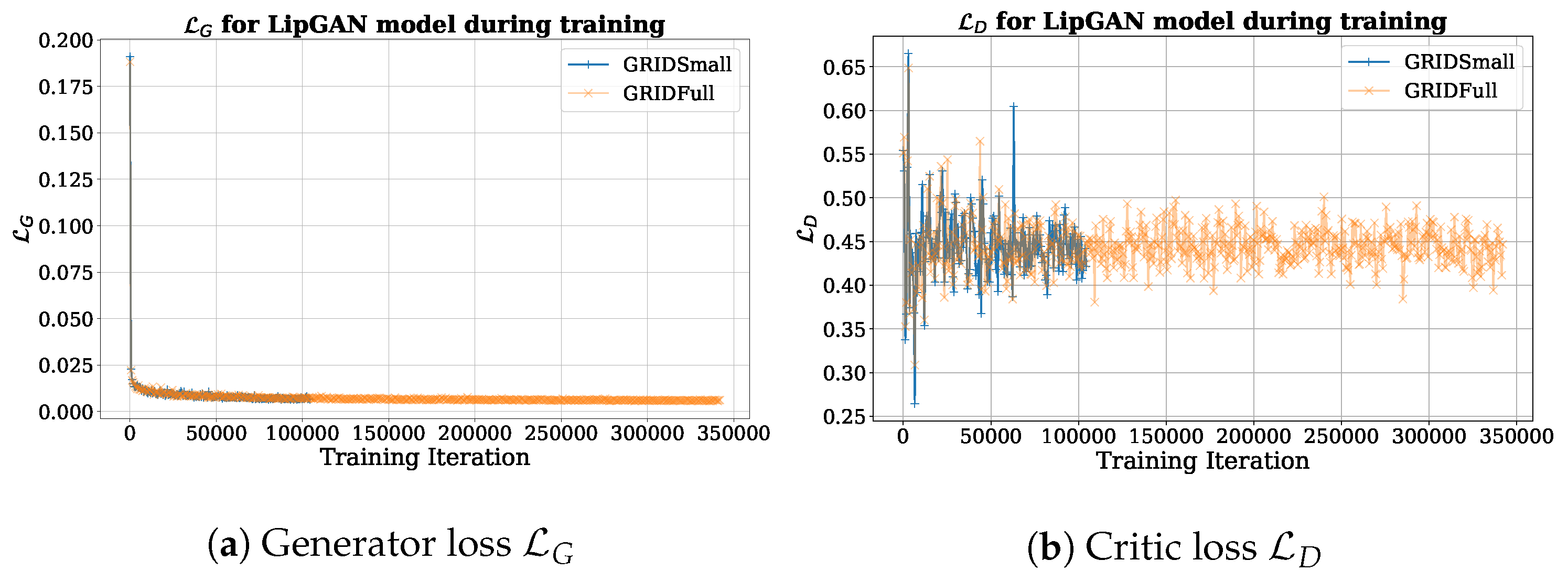
The LipGAN model was trained using the GRIDSmall and the GRIDFull datasets for 20 epochs. This took approximately 1 day with 105,000 training iterations for GRIDSmall and 3 days with 342,400 training iterations for GRIDFull, on both systems. During training, the different LipGAN losses were sampled every 600th training iteration for both datasets. As displayed in Figure 2, the generator loss L G converges to around 0, with a minimum loss of 6.0 × 10 3 for GRIDSmall and 5.7 × 10 3 for GRIDFull. The discriminator loss L D converges around 0.45; however, some outliers can be seen, which resulted in a search for potential errors in the training samples, although none were found. Additionally, the loss L face with the input of a fake face S ^ with real audio A, and the loss L audio with the input of a real face S but time-unsynced audio A , were sampled. This was performed even if they did not contribute to the discriminator loss L D for that specific iteration. These losses can be seen in Figure 3. Despite some outliers for the loss L audio , both losses seem to converge, although this process is slower for L audio than L face .
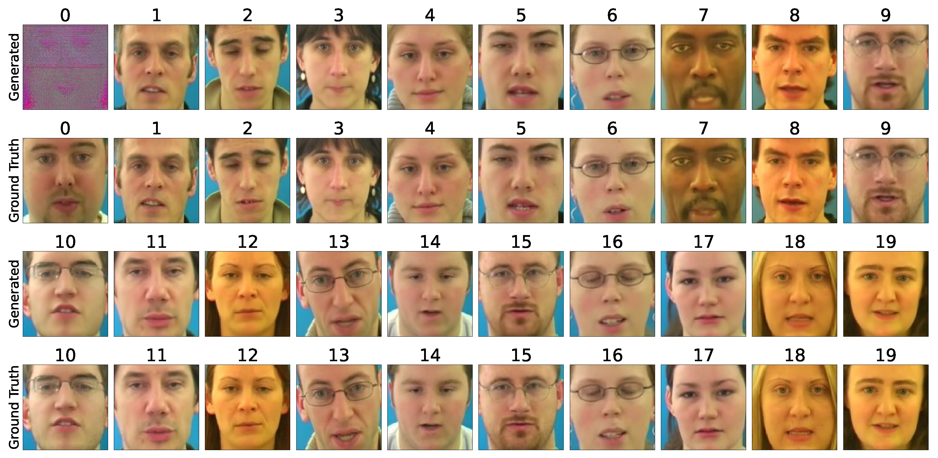
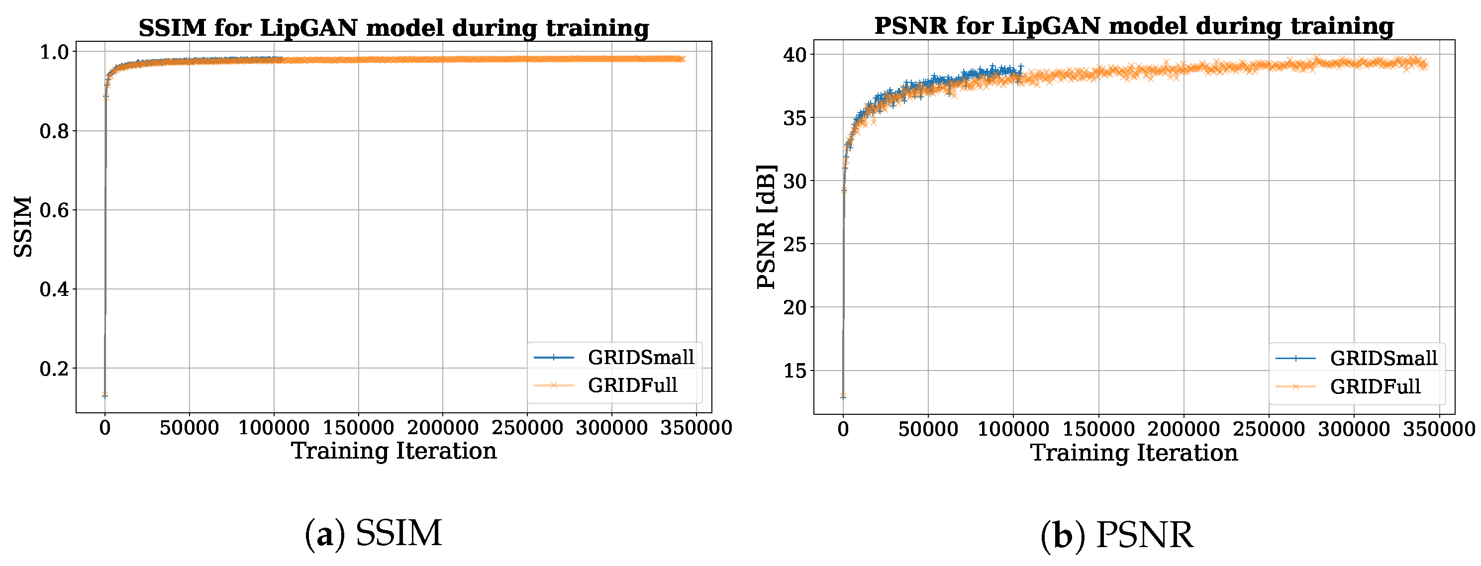
Sample inspection. Most generated faces are of good quality after the first epoch. However, if one looks closely, small differences for some select samples can be seen in the samples in Figure 4. For example, in the sample for epoch 7, one can see that the generator produces a face with an open mouth, while the mouth is more closed for the ground truth face. Further, for sample 9, one can notice that the beard has a more blurry appearance than its ground truth counterpart. Lastly, the SSIM and PSNR were calculated for the generator’s samples, together with the ground truth counterpart, every 600th training iteration. This can be seen in Figure 5.
Quality metrics. For convenience, we plot the SSIM and PSNR scores for our LipGAN implementation, once with the reduced dataset GRIDSmall and once for GRIDFull. The SSIM ranges from around 0.13 to 0.98 for both datasets, the PSNR starts at around 13 dB for both datasets, and the end is at about 39 dB for GRIDSmall and 40 dB for GRIDFull.

5.2. Experiments with L1WGAN-GP

In a second round of experiments, we implemented our L1WGAN-GP model, described in Section 3. As explained above, due to the fact that the penalty terms for each discriminator input x ^ are calculated individually, batch normalization can not be used.
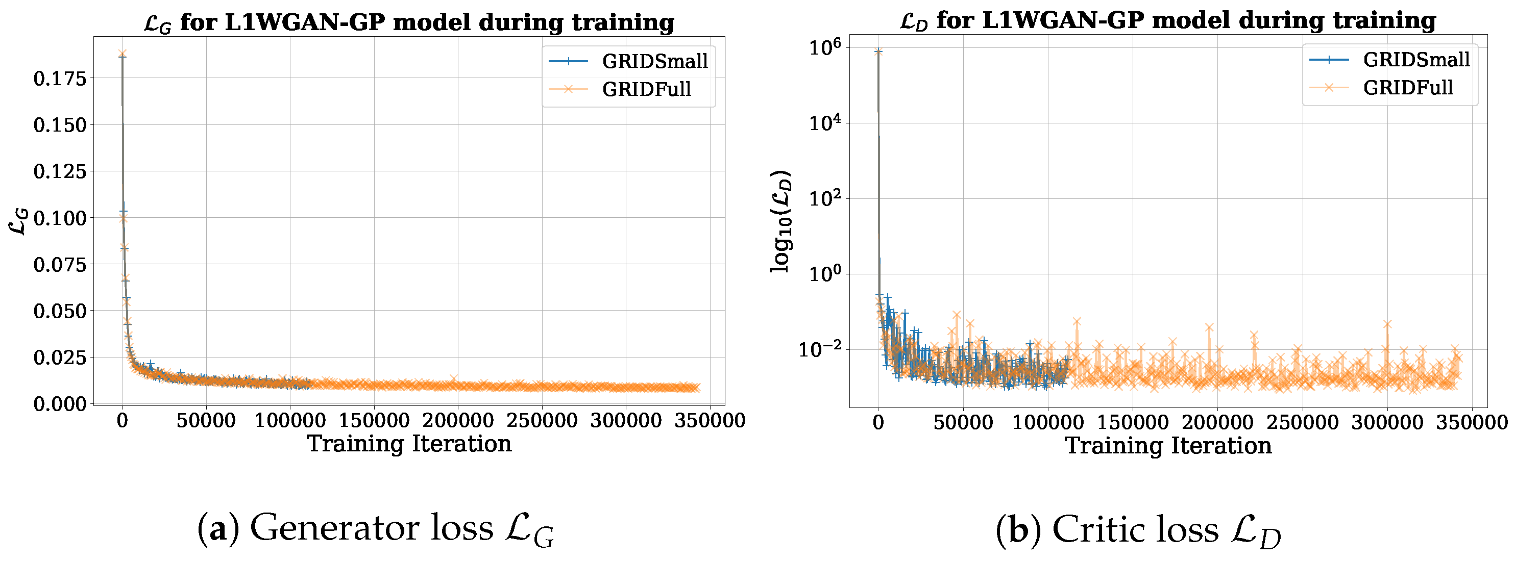
Let us briefly outline the major differences between the WGAN model and the LipGAN model during the training process: For each training step, the WGAN model trained the discriminator every step, and the generator every 5th step, using backpropagation. L1WGAN-GP was trained on the GRIDSmall and the GRIDFull dataset for 20 epochs, which resulted in 105,000 training iterations and 342,400 training iterations, respectively. To check convergence, we sampled the generator loss L G and the discriminator loss L D at the 600th training iteration, visualized in Figure 6, as well as the gradient penalty term R GP , plotted in Figure 7.
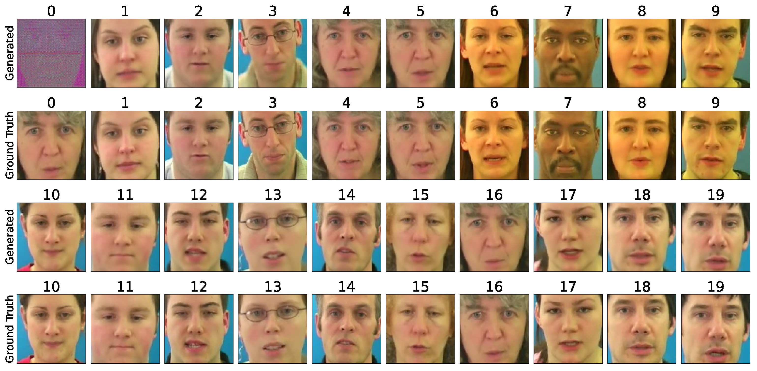
Sample inspection. Samples for the generated faces S ^ and their corresponding ground truth part S were saved once per epoch during the training. We see in Figure 8 that the samples have a realistic look but tend to be slightly blurry at times, especially for the early epochs. Upon inference, the model produced distinct faces for each separate frame, and no sign of suspected mode collapse could be observed.
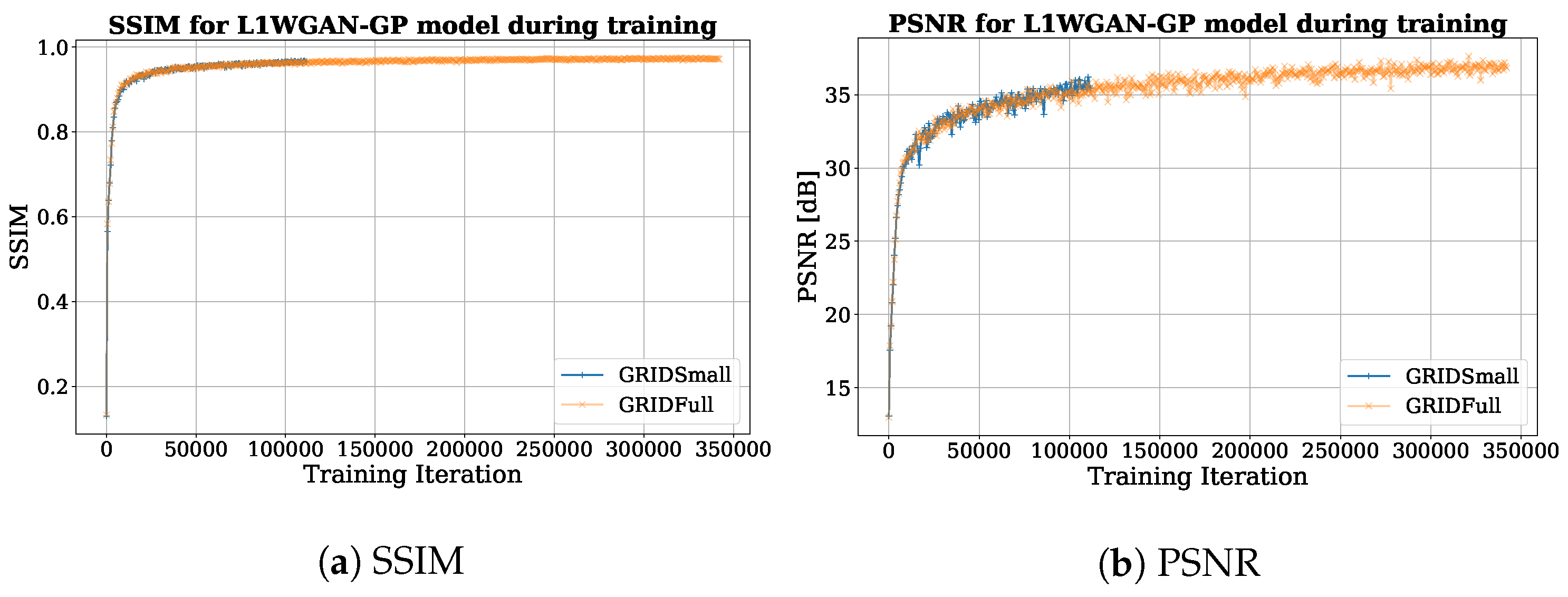
Quality metrics. As visualized in Figure 9, the SSIM goes from approximately 0.13 for both models to 0.97 and 0.98 for GRIDSmall and GRIDFull, respectively. Further, the PSNR ranges from around 13 dB for both datasets to around 36 dB for GRIDSmall and 37 dB for GRIDFull.

6. Results

In this section we summarize the results of our experiments. The motivation for our work was the animation of an image, showing a portrait snippet of a single person on a “good” background, in a short video message with prescribed audio. We mimic an everyday application setting by using only mild computational resources and openly available datasets for our task. For this aim, the GRID dataset seemed to be most adapted, given (a) its controlled setting and (b) its annotated audio transcription, making it most convenient for a later implementation of a text-to-speech feature.

6.1. Dataset Impact on LipGAN

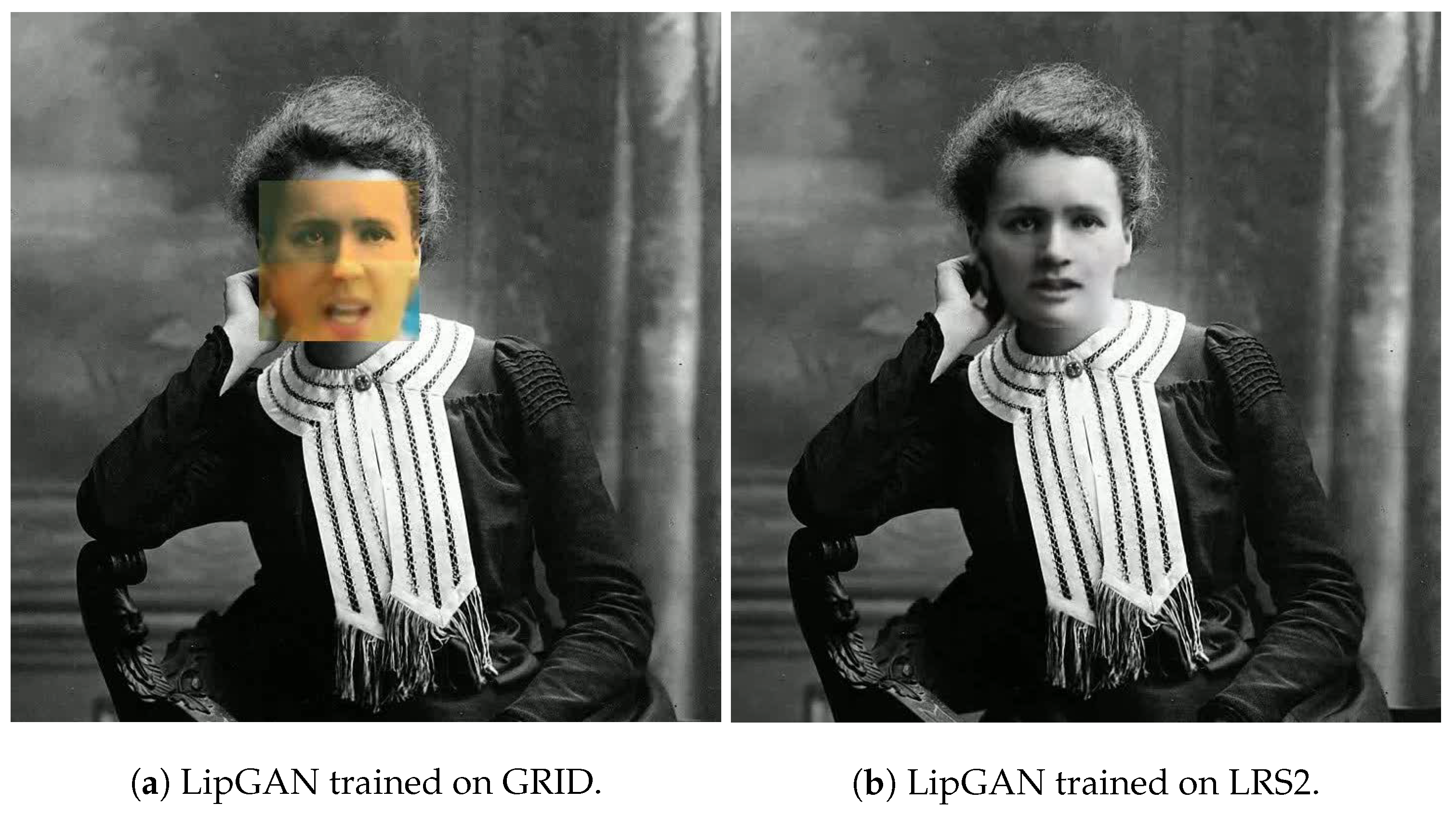
A first surprising outcome is the poor generalization of our reimplemented Pytorch LipGAN to grayscale images. While the original Keras-LipGAN model trained on LRS2 gave satisfactory visual results after inference, the Pytorch-LipGAN model trained on GRID did not manage to adapt to the new color scheme, as showcased in Figure 10. One might also speculate whether the mouth is slightly misplaced and slightly larger than it should be.
We conclude that the outcome of inference is sensitive depending on the properties of the used target data. This problem is typical for GAN algorithms and also discussed by [79], whose model performance is also limited to quite controlled settings of well-aligned frontal faces, such as in GRID.
Further studies on a data-augmented GRID dataset with additional grayscale images should be performed to investigate the issue and see if it can be remedied for LipGAN trained on GRID.

6.2. FID, SSIM, and PSNR Scores

We compare LipGAN and L1WGAN-GP in terms of three quantitative metrics, FID, SSIM, and PSNR, evaluated on unseen test data, in the form of the GRIDTest dataset. All scores used the 44,589 points of reference data in TestGRID; the SSIM and PSNR are visualized as boxplots with outliers omitted for better visibility. The results of the FID score are presented in Table 3. Here, the L1WGAN-GP model outperforms our reimplementation of LipGAN, signifying that, for L1WGAN-GP, the generated data distribution is closer to the reference data distribution.
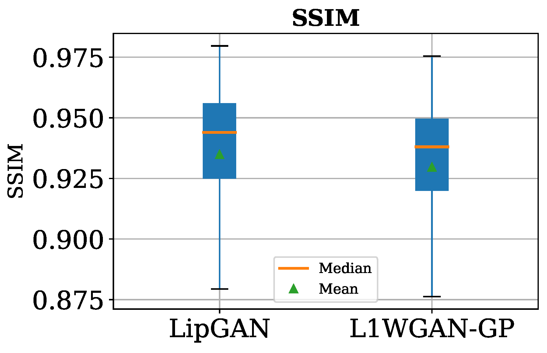
The SSIM was evaluated for each of the 44589 data points in GRIDTest and the result of this, in the form of a box plot, can be seen in Figure 11. Note that the box plot does not include outliers to make the box more visible. In terms of the SSIM, both LipGAN and L1WGAN-GP reach values close to the maximum possible value of 1.0 , with LipGAN performing slightly better than L1WGAN-GP in terms of both the median and mean value. Table 4 summarizes the numeric properties of the acquired SSIM scores.
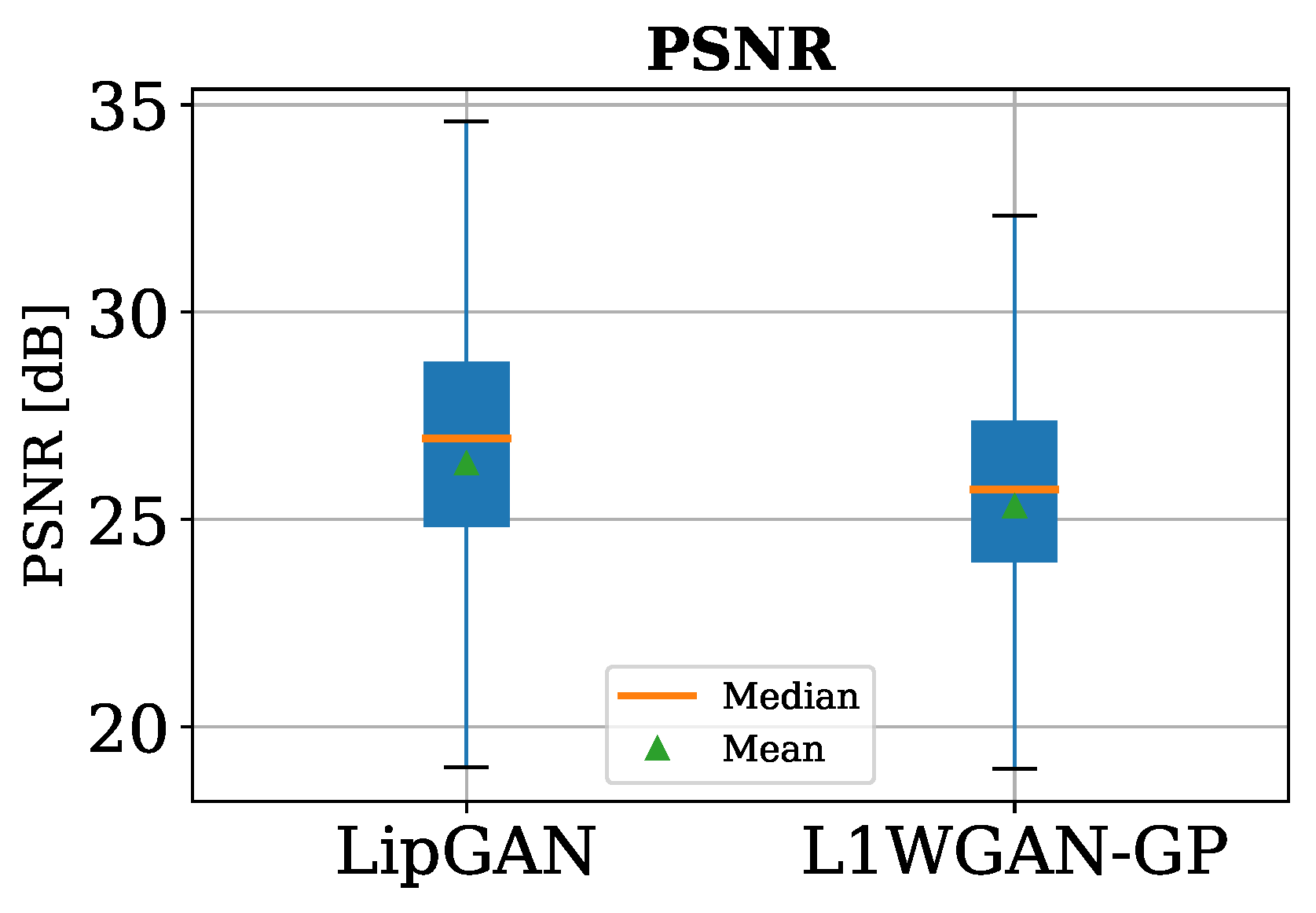
Similar to the SSIM, PSNR was evaluated for all 44,589 data points in GRIDTest and the result is presented as a box plot in Figure 12.
For the PSNR, we see a very different phenomenon: first, the spread was quite large, ranging around 15 dB, and LipGAN outperformed L1WGAN-GP in terms of the median and mean. As in the comparison of SSIM, the outliers of the box plot were been omitted. A summary of the numerical properties of the box plot can be seen in Table 5, which again confirms the box plot.

6.3. Qualitative Comparison

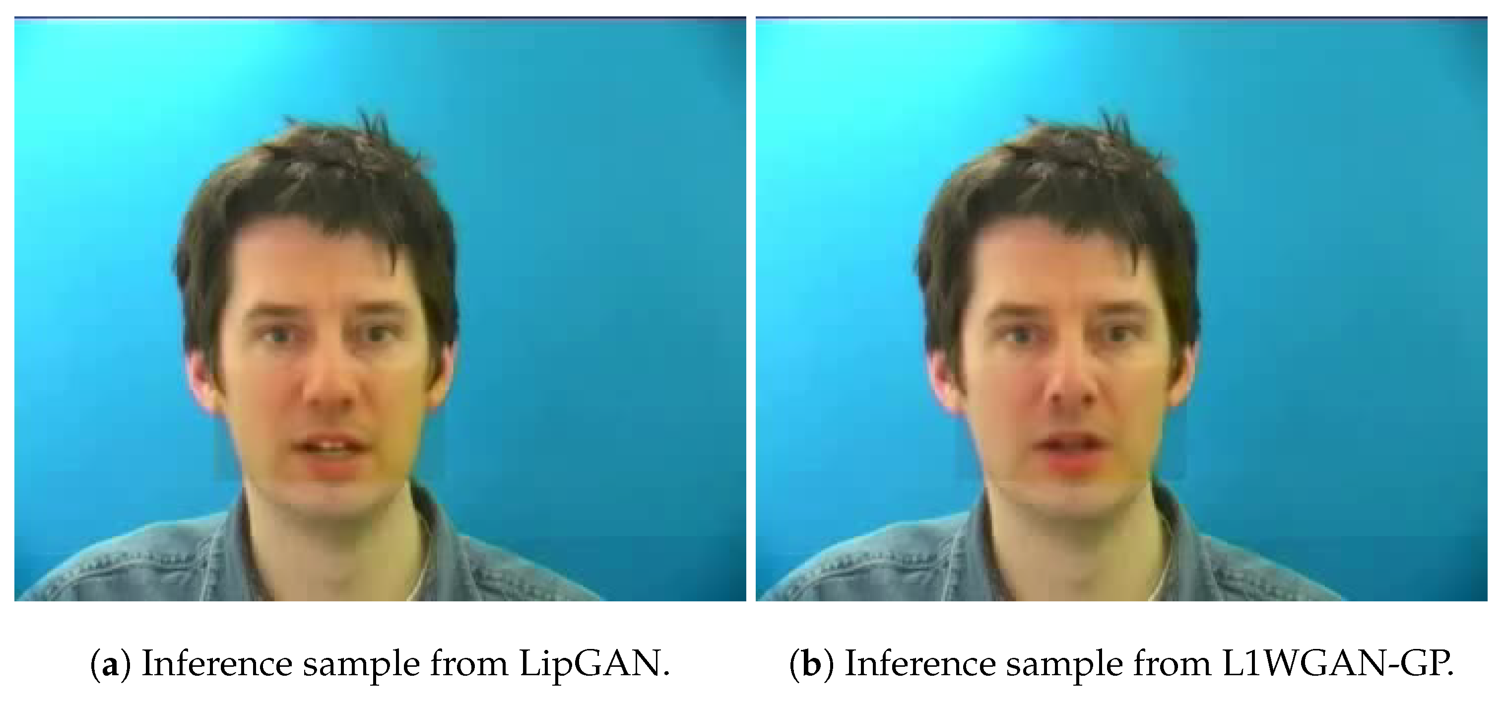
We further examine some qualitative aspects of the two models by looking at the generated data produced by using GRIDTrain as input. As a first remark, it should be highlighted that both models solved the task of lip synchronization adequately good in a subjective manner. We note upon inspection of the data produced during inference, of both models, a certain discrepancy between the generated face and the background. This can be noticed as a visible box surrounding the face. This phenomenon was noticed equally much for both models and is displayed in Figure 13.
Additionally, some of the images produced by L1WGAN-GP had visual artifacts, see examples in Figure 14. This problem was not experienced in data produced by LipGAN.
The artifacts in L1WGAN-GP mostly occur around the eyes of the target face and appear visually in a variety of ways, as discolored pixels, in many cases matching the surrounding background, see Figure 14. The artifacts most likely originate from the fact that the L1WGAN-GP model fails to differentiate the background from certain areas of the face. It is difficult to determine why these artifacts appear when trained with GRID, which is a relatively controlled dataset. To some extent, artifacts are unavoidable when facial expressions need to be generated, as these always imply deviations from the ground truth. It could be that more training hours are needed, as the generator in L1WGAN-GP only begins updating every fifth iteration. However, this is ruled out by the quick convergence of losses and similar metric performance compared to LipGAN.

7. Conclusions and Outlook

To summarize, the quantitative metrics used were not very conclusive when comparing LipGAN and L1WGAN-GP. In all three cases, the results were numerically close to each other, while sample inspection did reveal flaws in L1WGAN-GP: a large number of artifacts were noticed in the images produced by the L1WGAN-GP model.
Considering the artifacts produced by L1WGAN-GP, one would have wished for a larger discrepancy in the quantitative metric scores. We guess that this did not happen as the metrics compare entire pictures; thus, a small artifact would not render a large difference in the metrics. In contrast to other applications, for the lip-synchronization task, which focuses on a quite small region in the image, even small artifacts can ruin the human-perceived image quality.
Furthermore, the focus of quantitative metrics on image quality and congruence with the ground truth makes them unsatisfactory for animation tasks, as it was outlined already by several authors.
While there is already no consensus about adequate quantitative metrics for GANs that output images, it seems to be even more challenging to determine a proper quantitative scoring system to measure the quality of video output.
In researchers’ attempts to make human-eye qualitative assessment more “standardized”, large-scale versions of the former were implemented, such as “online Turing tests” [79] or mean-opinion-score. For years, however, there have been warnings [80,81] that it is not clear what the MOS actually measures, as no dimensions of output quality and no standardization of tester scores is ensured.
We conclude that there is currently no appropriate alternative to human inspection available to quantitatively measure the quality of lip synchronization, not because there would not be research on multidimensional quality measurement alternatives [81] but simply because a single number seems to be given preference to a more sophisticated analysis.

8. Responsible AI Considerations

While this research primarily addresses the theoretical underpinnings of speech-driven facial animation and the unsatisfactory results of currently used evaluation metrics, it is, of course, related to the design and deployment of generative models in multimedia systems. The ongoing efforts in creating audio-conditioned, lifelike talking-head avatars have applications beyond entertainment and virtual communication. It may enhance accessibility for individuals with speech or motor impairments through visually expressive assistive agents, expand the reach and engagement of educational content via interactive AI tutors, and support mental health interventions by enabling emotionally responsive virtual agents, as demonstrated in the related affective computing literature [82,83]. Despite the positive potential, generative audiovisual systems—especially those involving photorealistic facial synthesis—raise well-documented ethical and security concerns, including the risks of impersonation, disinformation, and non-consensual media creation [84,85,86,87]. Although the present study does not aim to facilitate such malicious uses, the underlying methods share inherent risks of “dual usage” common to deep generative frameworks. Several well-functioning forgery detection models were suggested, such as [88,89], based on a two-stream convolutional neural network (CNN) architecture.
Encouragingly, state-of-the-art detectors, such as those evaluated on synthetic content produced by models like Microsoft’s VASA-1 [90], continue to achieve high classification performance (e.g., 97.8% accuracy), indicating that detection is keeping pace with synthesis quality—at least in controlled settings. To further contribute to safe and accountable AI practices, the positive use of synthetic data in countering media forgery should be encouraged and intensified, aligning with recent research advocating for synthetic augmentation as a viable strategy for improving deepfake detection performance [91,92].
As summarized in Section 2, the output of current talking-head generation models still contains visual artifacts that distinguish it from real footage, which mitigates immediate risk of misuse. Nevertheless, as generative quality improves, transparency, external auditing, and clear model disclosure will be critical in mitigating harms and guiding the responsible integration of such technologies into society [93]. For a discussion on the necessary requirements for high-risk AI systems, see, e.g., [94].

Author Contributions

Methodology, J.L. and P.N.; Software, J.L. and P.N.; Investigation, C.G.; Writing—original draft, C.G.; Writing—review & editing, C.G.; Supervision, C.G.; Project administration, C.G. All authors contributed equally to this work. All authors have read and agreed to the published version of the manuscript.

Funding

This research received no external funding.

Data Availability Statement

The original data presented in the study are openly available in the Zenodo repository https://zenodo.org/records/3625687, last accessed on 1 August 2025.

Acknowledgments

P.N. and J.L. thank Sinch AB Malmö lab for providing computational resources.

Conflicts of Interest

The authors declare no conflicts of interest.

References

  1. Simons, A.; Cox, S. Generation of Mouthshape for a Synthetic Talking Head. In Proceedings of the Institute of Acoustics, 1990. Available online: https://www.researchgate.net/publication/243634521 (accessed on 1 August 2025).
  2. Tan, S.; Ji, B.; Bi, M.; Pan, Y. Edtalk: Efficient disentanglement for emotional talking head synthesis. In Proceedings of the European Conference on Computer Vision, Milan, Italy, 29 September–4 October 2024; Springer: Berlin/Heidelberg, Germany, 2024; pp. 398–416. [Google Scholar]
  3. Li, C.; Zhang, C.; Xu, W.; Lin, J.; Xie, J.; Feng, W.; Peng, B.; Chen, C.; Xing, W. LatentSync: Taming Audio-Conditioned Latent Diffusion Models for Lip Sync with SyncNet Supervision. arXiv 2024, arXiv:2412.09262. [Google Scholar]
  4. Qi, J.; Ji, C.; Xu, S.; Zhang, P.; Zhang, B.; Bo, L. Chatanyone: Stylized real-time portrait video generation with hierarchical motion diffusion model. arXiv 2025, arXiv:2503.21144. [Google Scholar]
  5. Ma, J.; Wang, S.; Yang, J.; Hu, J.; Liang, J.; Lin, G.; Chen, J.; Li, K.; Meng, Y. Sayanything: Audio-driven lip synchronization with conditional video diffusion. arXiv 2025, arXiv:2502.11515. [Google Scholar]
  6. Zhang, Y.; Zhong, Z.; Liu, M.; Chen, Z.; Wu, B.; Zeng, Y.; Zhan, C.; He, Y.; Huang, J.; Zhou, W. MuseTalk: Real-Time High-Fidelity Video Dubbing via Spatio-Temporal Sampling. arXiv 2024, arXiv:2410.10122. [Google Scholar]
  7. Feng, G.; Ma, Z.; Li, Y.; Jing, J.; Yang, J.; Miao, Q. FaceEditTalker: Interactive Talking Head Generation with Facial Attribute Editing. arXiv 2025, arXiv:2505.22141. [Google Scholar]
  8. Kim, J.; Cho, J.; Park, J.; Hwang, S.; Kim, D.E.; Kim, G.; Yu, Y. DEEPTalk: Dynamic Emotion Embedding for Probabilistic Speech-Driven 3D Face Animation. In Proceedings of the AAAI Conference on Artificial Intelligence, Philadelphia, PA, USA, 25 February–4 March 2025; Volume 39, pp. 4275–4283. [Google Scholar]
  9. Jang, Y.; Kim, J.H.; Ahn, J.; Kwak, D.; Yang, H.S.; Ju, Y.C.; Kim, I.H.; Kim, B.Y.; Chung, J.S. Faces that speak: Jointly synthesising talking face and speech from text. In Proceedings of the IEEE/CVF Conference on Computer Vision and Pattern Recognition, Seattle, WA, USA, 16–22 June 2024; pp. 8818–8828. [Google Scholar]
  10. Mukhopadhyay, S.; Suri, S.; Gadde, R.T.; Shrivastava, A. Diff2lip: Audio conditioned diffusion models for lip-synchronization. In Proceedings of the IEEE/CVF Winter Conference on Applications of Computer Vision, Waikoloa, HI, USA, 3–8 January 2024; pp. 5292–5302. [Google Scholar]
  11. Lin, W. Enhancing Video Conferencing Experience through Speech Activity Detection and Lip Synchronization with Deep Learning Models. J. Comput. Technol. Appl. Math. 2025, 2, 16–23. [Google Scholar] [CrossRef]
  12. Peng, Z.; Liu, J.; Zhang, H.; Liu, X.; Tang, S.; Wan, P.; Zhang, D.; Liu, H.; He, J. Omnisync: Towards universal lip synchronization via diffusion transformers. arXiv 2025, arXiv:2505.21448. [Google Scholar] [CrossRef]
  13. Liu, L.; Wang, J.; Chen, S.; Li, Z. VividWav2Lip: High-fidelity facial animation generation based on speech-driven lip synchronization. Electronics 2024, 13, 3657. [Google Scholar] [CrossRef]
  14. Jiang, J.; Alwan, A.; Keating, P.A.; Auer, E.T., Jr.; Bernstein, L.E. On the relationship between face movements, tongue movements, and speech acoustics. EURASIP J. Adv. Signal Process. 2002, 2002, 506945. [Google Scholar] [CrossRef]
  15. Haider, C.L.; Park, H.; Hauswald, A.; Weisz, N. Neural speech tracking highlights the importance of visual speech in multi-speaker situations. J. Cogn. Neurosci. 2024, 36, 128–142. [Google Scholar] [CrossRef]
  16. Thies, J.; Zollhofer, M.; Stamminger, M.; Theobalt, C.; Nießner, M. Face2face: Real-time face capture and reenactment of rgb videos. In Proceedings of the IEEE Conference on Computer Vision and Pattern Recognition, Las Vegas, NV, USA, 27–30 June 2016; pp. 2387–2395. [Google Scholar]
  17. Alshahrani, M.H.; Maashi, M.S. A Systematic Literature Review: Facial Expression and Lip Movement Synchronization of an Audio Track. IEEE Access 2024, 12, 75220–75237. [Google Scholar] [CrossRef]
  18. Kadam, A.; Rane, S.; Mishra, A.K.; Sahu, S.K.; Singh, S.; Pathak, S.K. A Survey of Audio Synthesis and Lip-syncing for Synthetic Video Generation. EAI Endorsed Trans. Creat. Technol. 2021, 8, 1–9. [Google Scholar] [CrossRef]
  19. Xie, L.; Liu, Z.Q. Realistic mouth-synching for speech-driven talking face using articulatory modelling. IEEE Trans. Multimed. 2007, 9, 500–510. [Google Scholar]
  20. Wang, L.; Qian, X.; Han, W.; Soong, F.K. Synthesizing photo-real talking head via trajectory-guided sample selection. In Proceedings of the Eleventh Annual Conference of the International Speech Communication Association, Chiba, Japan, 26–30 September 2010. [Google Scholar]
  21. Llorach, G.; Evans, A.; Blat, J.; Grimm, G.; Hohmann, V. Web-based live speech-driven lip-sync. In Proceedings of the 2016 8th International Conference on Games and Virtual Worlds for Serious Applications (VS-GAMES), Barcelona, Spain, 7–9 September 2016; IEEE: Piscataway Township, NJ, USA, 2016; pp. 1–4. [Google Scholar]
  22. Fan, B.; Wang, L.; Soong, F.K.; Xie, L. Photo-real talking head with deep bidirectional LSTM. In Proceedings of the 2015 IEEE International Conference on Acoustics, Speech and Signal Processing (ICASSP), South Brisbane, Australia, 19–24 April 2015; IEEE: Piscataway Township, NJ, USA, 2015; pp. 4884–4888. [Google Scholar]
  23. Liu, Z.; Yeh, R.A.; Tang, X.; Liu, Y.; Agarwala, A. Video frame synthesis using deep voxel flow. In Proceedings of the IEEE International Conference on Computer Vision, Venice, Italy, 22–29 October 2017; pp. 4463–4471. [Google Scholar]
  24. Wiles, O.; Koepke, A.; Zisserman, A. X2face: A network for controlling face generation using images, audio, and pose codes. In Proceedings of the European Conference on Computer Vision (ECCV), Munich, Germany, 8–14 September 2018; pp. 670–686. [Google Scholar]
  25. Hong, F.T.; Zhang, L.; Shen, L.; Xu, D. Depth-aware generative adversarial network for talking head video generation. In Proceedings of the IEEE/CVF Conference on Computer Vision and Pattern Recognition, New Orleans, LA, USA, 18–24 June 2022; pp. 3397–3406. [Google Scholar]
  26. Bounareli, S.; Tzelepis, C.; Argyriou, V.; Patras, I.; Tzimiropoulos, G. One-shot neural face reenactment via finding directions in gan’s latent space. Int. J. Comput. Vis. 2024, 132, 3324–3354. [Google Scholar] [CrossRef]
  27. Su, J.; Liu, K.; Chen, L.; Yao, J.; Liu, Q.; Lv, D. Audio-driven high-resolution seamless talking head video editing via stylegan. In Proceedings of the 2024 IEEE International Conference on Multimedia and Expo (ICME), Niagara Falls, ON, Canada, 15–19 July 2024; IEEE: Piscataway Township, NJ, USA, 2024; pp. 1–6. [Google Scholar]
  28. Zia, R.; Rehman, M.; Hussain, A.; Nazeer, S.; Anjum, M. Improving synthetic media generation and detection using generative adversarial networks. PeerJ Comput. Sci. 2024, 10, e2181. [Google Scholar] [CrossRef]
  29. Barthel, F.; Morgenstern, W.; Hinzer, P.; Hilsmann, A.; Eisert, P. CGS-GAN: 3D Consistent Gaussian Splatting GANs for High Resolution Human Head Synthesis. arXiv 2025, arXiv:2505.17590. [Google Scholar] [CrossRef]
  30. Doukas, M.C.; Zafeiriou, S.; Sharmanska, V. Headgan: One-shot neural head synthesis and editing. In Proceedings of the IEEE/CVF International Conference on Computer Vision, Montreal, BC, Canada, 11–17 October 2021; pp. 14398–14407. [Google Scholar]
  31. Ma, F.; Xie, Y.; Li, Y.; He, Y.; Zhang, Y.; Ren, H.; Liu, Z.; Yao, W.; Ren, F.; Yu, F.R.; et al. A review of human emotion synthesis based on generative technology. IEEE Trans. Affect. Comput. 2025; early access. [Google Scholar] [CrossRef]
  32. Suwajanakorn, S.; Seitz, S.M.; Kemelmacher-Shlizerman, I. Synthesizing Obama: Learning lip sync from audio. ACM Trans. Graph. (ToG) 2017, 36, 1–13. [Google Scholar] [CrossRef]
  33. Kumar, R.; Sotelo, J.; Kumar, K.; de Brebisson, A.; Bengio, Y. ObamaNet: Photo-realistic lip-sync from text. arXiv 2017, arXiv:1801.01442. [Google Scholar] [CrossRef]
  34. Jamaludin, A.; Chung, J.S.; Zisserman, A. You said that?: Synthesising talking faces from audio. Int. J. Comput. Vis. 2019, 127, 1767–1779. [Google Scholar] [CrossRef]
  35. Prajwal, K.; Mukhopadhyay, R.; Namboodiri, V.P.; Jawahar, C. A lip sync expert is all you need for speech to lip generation in the wild. In Proceedings of the 28th ACM International Conference on Multimedia, Seattle, WA, USA, 12–16 October 2020; pp. 484–492. [Google Scholar]
  36. Afouras, T.; Chung, J.S.; Senior, A.; Vinyals, O.; Zisserman, A. Deep Audio-visual Speech Recognition. IEEE Trans. Pattern Anal. Mach. Intell. 2019, 4, 8717–8727. [Google Scholar] [CrossRef] [PubMed]
  37. Prajwal, K.R.; Mukhopadhyay, R.; Jerin, P.; Abhishek, J.; Namboodiri, V.; Jawahar, C.V. Towards Automatic Face-to-Face Translation. In Proceedings of the 27th ACM International Conference on Multimedia, Nice, France, 21–25 October 2019; MM ’19. pp. 1428–1436. [Google Scholar] [CrossRef]
  38. Park, S.J.; Kim, M.; Hong, J.; Choi, J.; Ro, Y.M. Synctalkface: Talking face generation with precise lip-syncing via audio-lip memory. In Proceedings of the AAAI Conference on Artificial Intelligence, Virtual, 22 February–1 March 2022; Volume 36, pp. 2062–2070. [Google Scholar]
  39. Xu, C.; Liu, Y.; Xing, J.; Wang, W.; Sun, M.; Dan, J.; Huang, T.; Li, S.; Cheng, Z.Q.; Tai, Y.; et al. Facechain-imagineid: Freely crafting high-fidelity diverse talking faces from disentangled audio. In Proceedings of the IEEE/CVF Conference on Computer Vision and Pattern Recognition, Seattle, WA, USA, 16–22 June 2024; pp. 1292–1302. [Google Scholar]
  40. Cheng, K.; Cun, X.; Zhang, Y.; Xia, M.; Yin, F.; Zhu, M.; Wang, X.; Wang, J.; Wang, N. Videoretalking: Audio-based lip synchronization for talking head video editing in the wild. In Proceedings of the SIGGRAPH Asia 2022 Conference Papers, Daegu, Republic of Korea, 6–9 December 2022; pp. 1–9. [Google Scholar]
  41. Tan, S.; Ji, B.; Pan, Y. Flowvqtalker: High-quality emotional talking face generation through normalizing flow and quantization. In Proceedings of the IEEE/CVF Conference on Computer Vision and Pattern Recognition, Seattle, WA, USA, 16–22 June 2024; pp. 26317–26327. [Google Scholar]
  42. Wu, X.; Hu, P.; Wu, Y.; Lyu, X.; Cao, Y.P.; Shan, Y.; Yang, W.; Sun, Z.; Qi, X. Speech2lip: High-fidelity speech to lip generation by learning from a short video. In Proceedings of the IEEE/CVF International Conference on Computer Vision, Paris, France, 1–6 October 2023; pp. 22168–22177. [Google Scholar]
  43. Wang, J.; Zhao, K.; Zhang, S.; Zhang, Y.; Shen, Y.; Zhao, D.; Zhou, J. Lipformer: High-fidelity and generalizable talking face generation with a pre-learned facial codebook. In Proceedings of the IEEE/CVF Conference on Computer Vision and Pattern Recognition, Vancouver, BC, Canada, 17–24 June 2023; pp. 13844–13853. [Google Scholar]
  44. Aneja, S.; Thies, J.; Dai, A.; Nießner, M. Facetalk: Audio-driven motion diffusion for neural parametric head models. In Proceedings of the IEEE/CVF Conference on Computer Vision and Pattern Recognition, Seattle, WA, USA, 16–22 June 2024; pp. 21263–21273. [Google Scholar]
  45. Wang, S.; Li, L.; Ding, Y.; Fan, C.; Yu, X. Audio2head: Audio-driven one-shot talking-head generation with natural head motion. arXiv 2021, arXiv:2107.09293. [Google Scholar]
  46. Yao, X.; Fried, O.; Fatahalian, K.; Agrawala, M. Iterative text-based editing of talking-heads using neural retargeting. ACM Trans. Graph. (TOG) 2021, 40, 1–14. [Google Scholar] [CrossRef]
  47. Zhou, H.; Liu, Y.; Liu, Z.; Luo, P.; Wang, X. Talking face generation by adversarially disentangled audio-visual representation. In Proceedings of the AAAI Conference on Artificial Intelligence, Honolulu, HI, USA, 27 January–1 February 2019; Volume 33, pp. 9299–9306. [Google Scholar]
  48. Chung, J.S.; Jamaludin, A.; Zisserman, A. You said that? arXiv 2017, arXiv:1705.02966. [Google Scholar] [CrossRef]
  49. Chen, L.; Li, Z.; Maddox, R.K.; Duan, Z.; Xu, C. Lip movements generation at a glance. In Proceedings of the European Conference on Computer Vision (ECCV), Munich, Germany, 8–14 September 2018; pp. 520–535. [Google Scholar]
  50. Stypułkowski, M.; Vougioukas, K.; He, S.; Zięba, M.; Petridis, S.; Pantic, M. Diffused heads: Diffusion models beat gans on talking-face generation. In Proceedings of the IEEE/CVF Winter Conference on Applications of Computer Vision, Waikoloa, HI, USA, 3–8 January 2024; pp. 5091–5100. [Google Scholar]
  51. Fan, X.; Gao, H.; Chen, Z.; Chang, P.; Han, M.; Hasegawa-Johnson, M. SyncDiff: Diffusion-Based Talking Head Synthesis with Bottlenecked Temporal Visual Prior for Improved Synchronization. In Proceedings of the 2025 IEEE/CVF Winter Conference on Applications of Computer Vision (WACV), Tucson, AZ, USA, 26 February–6 March 2025; IEEE: Piscataway Township, NJ, USA, 2025; pp. 4554–4563. [Google Scholar]
  52. Li, T.; Zheng, R.; Yang, M.; Chen, J.; Yang, M. Ditto: Motion-space diffusion for controllable realtime talking head synthesis. arXiv 2024, arXiv:2411.19509. [Google Scholar] [CrossRef]
  53. Cheng, H.; Lin, L.; Liu, C.; Xia, P.; Hu, P.; Ma, J.; Du, J.; Pan, J. DAWN: Dynamic Frame Avatar with Non-autoregressive Diffusion Framework for Talking Head Video Generation. arXiv 2024, arXiv:2410.13726. [Google Scholar] [CrossRef]
  54. Mir, A.; Alonso, E.; Mondragón, E. DiT-Head: High Resolution Talkin Head Synthesis using Diffusion Transformers. In Proceedings of the 16th International Conference on Agents and Artificial Intelligence, Rome, Italy, 24–26 February 2024; Volume 3, pp. 159–169. [Google Scholar]
  55. Chopin, B.; Dhamija, T.; Balaji, P.; Wang, Y.; Dantcheva, A. Dimitra: Audio-driven Diffusion model for Expressive Talking Head Generation. arXiv 2025, arXiv:2502.17198. [Google Scholar]
  56. Ma, Z.; Zhu, X.; Qi, G.; Qian, C.; Zhang, Z.; Lei, Z. Diffspeaker: Speech-driven 3d facial animation with diffusion transformer. arXiv 2024, arXiv:2402.05712. [Google Scholar]
  57. Rakesh, V.K.; Mazumdar, S.; Maity, R.P.; Pal, S.; Das, A.; Samanta, T. Advancing Talking Head Generation: A Comprehensive Survey of Multi-Modal Methodologies, Datasets, Evaluation Metrics, and Loss Functions. arXiv 2025, arXiv:2507.02900. [Google Scholar]
  58. Xue, H.; Luo, X.; Hu, Z.; Zhang, X.; Xiang, X.; Dai, Y.; Liu, J.; Zhang, Z.; Li, M.; Yang, J.; et al. Human motion video generation: A survey. IEEE Trans. Pattern Anal. Mach. Intell. 2025; early access. [Google Scholar] [CrossRef]
  59. Zhou, Y.; Han, X.; Shechtman, E.; Echevarria, J.; Kalogerakis, E.; Li, D. Makelttalk: Speaker-aware talking-head animation. ACM Trans. Graph. (TOG) 2020, 39, 1–15. [Google Scholar] [CrossRef]
  60. Zhou, H.; Sun, Y.; Wu, W.; Loy, C.C.; Wang, X.; Liu, Z. Pose-controllable talking face generation by implicitly modularized audio-visual representation. In Proceedings of the IEEE/CVF Conference on Computer Vision and Pattern Recognition, Nashville, TN, USA, 20–25 June 2021; pp. 4176–4186. [Google Scholar]
  61. Zhang, W.; Cun, X.; Wang, X.; Zhang, Y.; Shen, X.; Guo, Y.; Shan, Y.; Wang, F. Sadtalker: Learning realistic 3d motion coefficients for stylized audio-driven single image talking face animation. In Proceedings of the IEEE/CVF Conference on Computer Vision and PATTERN Recognition, Vancouver, BC, Canada, 17–24 June 2023; pp. 8652–8661. [Google Scholar]
  62. Yin, F.; Zhang, Y.; Cun, X.; Cao, M.; Fan, Y.; Wang, X.; Bai, Q.; Wu, B.; Wang, J.; Yang, Y. Styleheat: One-shot high-resolution editable talking face generation via pre-trained stylegan. In Proceedings of the European Conference on Computer Vision, Milan, Italy, 29 September–4 October 2024; Springer: Berlin/Heidelberg, Germany, 2022; pp. 85–101. [Google Scholar]
  63. Xu, Q.; Huang, G.; Yuan, Y.; Guo, C.; Sun, Y.; Wu, F.; Weinberger, K. An empirical study on evaluation metrics of generative adversarial networks. arXiv 2018, arXiv:1806.07755. [Google Scholar] [CrossRef]
  64. Arjovsky, M.; Chintala, S.; Bottou, L. Wasserstein generative adversarial networks. In Proceedings of the International Conference on Machine Learning, PMLR, Sydney, Australia, 6–11 August 2017; pp. 214–223. [Google Scholar]
  65. Villani, C. Optimal Transport: Old and New; Springer: Berlin/Heidelberg, Germany, 2008; Volume 338. [Google Scholar]
  66. Gulrajani, I.; Ahmed, F.; Arjovsky, M.; Dumoulin, V.; Courville, A.C. Improved training of wasserstein gans. In Proceedings of the International Conference on Neural Information Processing Systems, Long Beach, CA, USA, 4–9 December 2017. [Google Scholar]
  67. Pinetz, T.; Soukup, D.; Pock, T. On the estimation of the Wasserstein distance in generative models. In Proceedings of the German Conference on Pattern Recognition, Konstanz, Germany, 27–30 September 2022; Springer: Berlin/Heidelberg, Germany, 2019; pp. 156–170. [Google Scholar]
  68. Miyato, T.; Kataoka, T.; Koyama, M.; Yoshida, Y. Spectral normalization for generative adversarial networks. arXiv 2018, arXiv:1802.05957. [Google Scholar] [CrossRef]
  69. Salimans, T.; Goodfellow, I.; Zaremba, W.; Cheung, V.; Radford, A.; Chen, X. Improved techniques for training gans. In Proceedings of the International Conference on Neural Information Processing Systems, Barcelona, Spain, 5–10 December 2016. [Google Scholar]
  70. Cooke, M.; Barker, J.; Cunningham, S.; Shao, X. An audio-visual corpus for speech perception and automatic speech recognition. J. Acoust. Soc. Am. 2006, 120, 2421–2424. [Google Scholar] [CrossRef] [PubMed]
  71. Kurach, K.; Lucic, M.; Zhai, X.; Michalski, M.; Gelly, S. A Large-Scale Study on Regularization and Normalization in GANs. arXiv 2019, arXiv:1807.04720. [Google Scholar] [CrossRef]
  72. Chong, M.J.; Forsyth, D. Effectively unbiased fid and inception score and where to find them. In Proceedings of the IEEE/CVF Conference on Computer Vision and Pattern Recognition, Seattle, WA, USA, 13–19 June 2020; pp. 6070–6079. [Google Scholar]
  73. Zhang, W.; Zhu, C.; Gao, J.; Yan, Y.; Zhai, G.; Yang, X. A comparative study of perceptual quality metrics for audio-driven talking head videos. In Proceedings of the 2024 IEEE International Conference on Image Processing (ICIP), Abu Dhabi, United Arab Emirates, 27–30 October 2024; IEEE: Piscataway Township, NJ, USA, 2024; pp. 1218–1224. [Google Scholar]
  74. Korhonen, J.; You, J. Peak signal-to-noise ratio revisited: Is simple beautiful? In Proceedings of the 2012 Fourth International Workshop on Quality of Multimedia Experience, Melbourne, Australia, 5–7 July 2012; IEEE: Piscataway Township, NJ, USA, 2012; pp. 37–38. [Google Scholar]
  75. Hore, A.; Ziou, D. Image quality metrics: PSNR vs. SSIM. In Proceedings of the 2010 20th International Conference on Pattern Recognition, Istanbul, Turkey, 23–26 August 2010; IEEE: Piscataway Township, NJ, USA, 2010; pp. 2366–2369. [Google Scholar]
  76. Avcıbaş, I.s.; Sankur, B.l.; Sayood, K. Statistical evaluation of image quality measures. J. Electron. Imaging 2002, 11, 206–223. [Google Scholar] [CrossRef]
  77. Wang, Z.; Bovik, A.C.; Sheikh, H.R.; Simoncelli, E.P. Image quality assessment: From error visibility to structural similarity. IEEE Trans. Image Process. 2004, 13, 600–612. [Google Scholar] [CrossRef]
  78. Heusel, M.; Ramsauer, H.; Unterthiner, T.; Nessler, B.; Hochreiter, S. Gans trained by a two time-scale update rule converge to a local nash equilibrium. In Proceedings of the International Conference on Neural Information Processing Systems, Long Beach, CA, USA, 4–9 December 2017. [Google Scholar]
  79. Vougioukas, K.; Petridis, S.; Pantic, M. Realistic speech-driven facial animation with gans. Int. J. Comput. Vis. 2020, 128, 1398–1413. [Google Scholar] [CrossRef]
  80. Viswanathan, M.; Viswanathan, M. Measuring speech quality for text-to-speech systems: Development and assessment of a modified mean opinion score (MOS) scale. Comput. Speech Lang. 2005, 19, 55–83. [Google Scholar] [CrossRef]
  81. Streijl, R.C.; Winkler, S.; Hands, D.S. Mean opinion score (MOS) revisited: Methods and applications, limitations and alternatives. Multimed. Syst. 2016, 22, 213–227. [Google Scholar] [CrossRef]
  82. Piferi, F. CHATCARE: An Emotional-Aware Conversational Agent for Assisted Therapy; POLITesi—Politecnico di Milano: Milan, Italy, 2022. [Google Scholar]
  83. Mensio, M.; Rizzo, G.; Morisio, M. The rise of emotion-aware conversational agents: Threats in digital emotions. In Proceedings of the Companion Proceedings of the The Web Conference 2018, Lyon, France, 23–27 April 2018; pp. 1541–1544. [Google Scholar]
  84. Chen, T.; Lin, J.; Yang, Z.; Qing, C.; Lin, L. Learning adaptive spatial coherent correlations for speech-preserving facial expression manipulation. In Proceedings of the IEEE/CVF Conference on Computer Vision and Pattern Recognition, Seattle, WA, USA, 16–22 June 2024; pp. 7267–7276. [Google Scholar]
  85. Mirsky, Y.; Lee, W. The creation and detection of deepfakes: A survey. ACM Comput. Surv. (CSUR) 2021, 54, 1–41. [Google Scholar] [CrossRef]
  86. Kietzmann, J.; Lee, L. Deepfakes: Trick or treat? Bus. Horizons 2020, 63, 135–146. [Google Scholar] [CrossRef]
  87. Khan, S.A.; Dang-Nguyen, D.T. Clipping the deception: Adapting vision-language models for universal deepfake detection. In Proceedings of the 2024 International Conference on Multimedia Retrieval, Phuket, Thailand, 10–14 June 2024; pp. 1006–1015. [Google Scholar]
  88. Yan, Z.; Yao, T.; Chen, S.; Zhao, Y.; Fu, X.; Zhu, J.; Luo, D.; Wang, C.; Ding, S.; Wu, Y.; et al. Df40: Toward next-generation deepfake detection. Adv. Neural Inf. Process. Syst. 2024, 37, 29387–29434. [Google Scholar]
  89. Kong, C.; Chen, B.; Li, H.; Wang, S.; Rocha, A.; Kwong, S. Detect and locate: Exposing face manipulation by semantic-and noise-level telltales. IEEE Trans. Inf. Forensics Secur. 2022, 17, 1741–1756. [Google Scholar] [CrossRef]
  90. Xu, S.; Chen, G.; Guo, Y.X.; Yang, J.; Li, C.; Zang, Z.; Zhang, Y.; Tong, X.; Guo, B. Vasa-1: Lifelike audio-driven talking faces generated in real time. Adv. Neural Inf. Process. Syst. 2024, 37, 660–684. [Google Scholar]
  91. Rössler, A.; Cozzolino, D.; Verdoliva, L.; Riess, C.; Thies, J.; Nießner, M. FaceForensics++: Learning to detect manipulated facial images. In Proceedings of the IEEE/CVF International Conference on Computer Vision, Seoul, Republic of Korea, 27 October–2 November 2019; pp. 1–11. [Google Scholar]
  92. Tolosana, R.; Vera-Rodriguez, R.; Fierrez, J.; Morales, A.; Ortega-Garcia, J. Deepfakes and beyond: A survey of face manipulation and fake detection. Inf. Fusion 2020, 64, 131–148. [Google Scholar] [CrossRef]
  93. Floridi, L.; Chiriatti, A. GPT-3: Its nature, scope, limits, and consequences. Minds Mach. 2020, 30, 681–694. [Google Scholar] [CrossRef]
  94. Siegel, D.; Kraetzer, C.; Seidlitz, S.; Dittmann, J. Media Forensic Considerations of the Usage of Artificial Intelligence Using the Example of DeepFake Detection. J. Imaging 2024, 10, 46. [Google Scholar] [CrossRef]
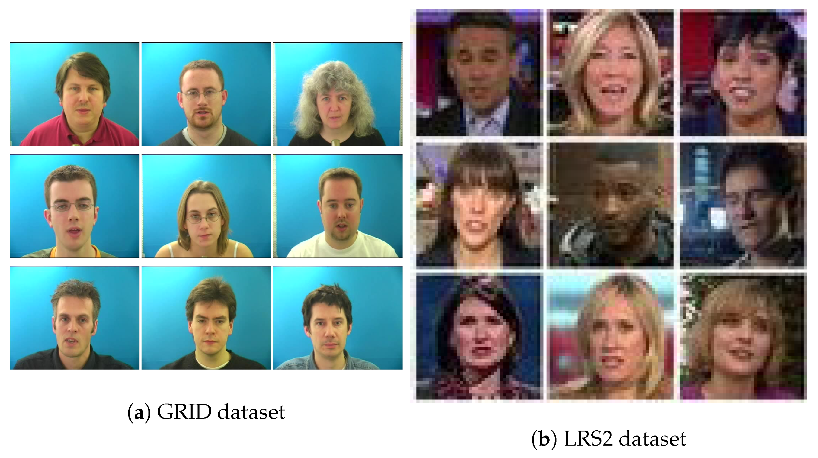
Figure 1. Samples of speakers from the datasets GRID [70] and LRS2 [36]. Note that the resolution in the LRS2 samples is not representative since it is a screenshot.
Electronics 14 03487 g001
Figure 2. Losses during training for the LipGAN model.
Electronics 14 03487 g002
Figure 3. Losses during training for the LipGAN model.
Electronics 14 03487 g003
Figure 4. Twenty random generated faces S ^ from the generator, together with their corresponding true faces S, from the training of the LipGAN model using GRIDFull. The number denotes the epoch.
Electronics 14 03487 g004
Figure 5. The metrics SSIM and PSNR for the LipGAN model during training. The metrics have been taken for every 600th training iteration.
Electronics 14 03487 g005
Figure 6. Losses during training for the WGAN-GP model.
Electronics 14 03487 g006
Figure 7. Gradient penalty term R GP for the L1WGAN-GP model.
Electronics 14 03487 g007
Figure 8. Twenty random generated faces S ^ from the generator, together with their corresponding true faces S, from the training of the L1WGAN-GP model using GRIDFull. The epoch for the samples is denoted by the number above each sample.
Electronics 14 03487 g008
Figure 9. The metrics SSIM and PSNR for the L1WGAN-GP model during training. The metrics have been taken for every 600th training iteration.
Electronics 14 03487 g009
Figure 10. Inference of LipGAN trained on two different datasets. The LipGAN model trained with GRID did not manage to adapt to the color scheme of the target image. Image source: Wikipedia.
Electronics 14 03487 g010
Figure 11. SSIM for the models trained on GRIDFull. Outliers have been omitted from the boxplot.
Electronics 14 03487 g011
Figure 12. PSNR for the models trained using GRIDFull. Outliers have been omitted from the boxplot.
Electronics 14 03487 g012
Figure 13. Example of a visual box surrounding the face during inference. This phenomenon occurred for both models.
Electronics 14 03487 g013
Figure 14. Example of visible artifacts from images produced by the L1WGAN-GP model with GRIDTrain as input.
Electronics 14 03487 g014
Table 1. Data attributes for the training data.
Data Attributes
Input image horizontal/vertical dimension H96
Frameshift time step α 1 , 2 , , 6
Mel-frequency channels M80
Mel-spectrogram time window T27
Table 2. Information about the data subsets used for all the experiments.
NameTypeIndividual SamplesVideos per Speaker
GRIDSmallTrain670,758300
GRIDFullTrain2,190,517980
GRIDTestTest44,58920
Table 3. FID score on the models trained using GRIDFull. Bold values indicate best performance.
ModelFID Score ↓
LipGAN15.11
L1WGAN-GP14.49
Table 4. SSIM summary statistics for the models trained on GRIDFull. Bold values indicate best performance.
ModelMean ↑Median ↑Max ↑Min ↑
LipGAN0.93480.94390.97960.7542
L1WGAN-GP0.92960.93800.97540.7052
Table 5. PSNR summary statistics for the models trained using GRIDFull.
ModelMean [dB] ↑Median [dB] ↑Max [dB] ↑Min [dB] ↑
LipGAN26.3426.9635.3513.67
L1WGAN-GP25.3225.7234.8412.81
Disclaimer/Publisher’s Note: The statements, opinions and data contained in all publications are solely those of the individual author(s) and contributor(s) and not of MDPI and/or the editor(s). MDPI and/or the editor(s) disclaim responsibility for any injury to people or property resulting from any ideas, methods, instructions or products referred to in the content.