Article

A Sequence-Aware Surrogate-Assisted Optimization Framework for Precision Gyroscope Assembly Based on AB-BiLSTM and SEG-HHO

School of Communication and Information Engineering, Nanjing University of Posts and Telecommunications, Nanjing 210003, China
*
Author to whom correspondence should be addressed.
Electronics 2025, 14(17), 3470; https://doi.org/10.3390/electronics14173470
Submission received: 19 July 2025 / Revised: 17 August 2025 / Accepted: 25 August 2025 / Published: 29 August 2025

Abstract

High-precision assembly plays a central role in aerospace, defense, and precision instrumentation, where errors in bolt preload or tightening sequences can directly degrade product reliability and lead to costly rework. Traditional finite element analysis (FEA) offers accuracy but is too computationally expensive for iterative or real-time optimization. Surrogate models are a promising alternative, yet conventional machine learning methods often neglect the sequential and constraint-aware nature of multi-bolt assembly. To overcome these limitations, this paper introduces an integrated framework that combines an Attention-based Bidirectional Long Short-Term Memory (AB-BiLSTM) surrogate with a stratified version of the Harris Hawks Optimizer (SEG-HHO). The AB-BiLSTM captures temporal dependencies in preload evolution while providing interpretability through attention–weight visualization, linking model focus to physical assembly dynamics. SEG-HHO employs an encoding–decoding mechanism to embed engineering constraints, enabling efficient search in complex and constrained design spaces. Validation on a gyroscope assembly task demonstrates that the framework achieves high predictive accuracy (Mean Absolute Error of 3.59 × 10⁻⁵), reduces optimization cost by orders of magnitude compared with FEA, and reveals physically meaningful patterns in bolt interactions. These results indicate a scalable and interpretable solution for precision assembly optimization.

1. Introduction

High-precision assembly is a critical process in high-technology manufacturing sectors such as aerospace, precision instrumentation, and defense systems. Even minor deviations in bolt torque or tightening sequence can lead to substantial performance degradation and costly rework. Industry analyses indicate that rework and scrap costs can account for 5–30% of total manufacturing costs, with up to 30% of equipment failures traced back to improper installation and assembly procedures [1]. In aerospace manufacturing, such assembly-related defects are among the leading causes of cost overruns. A recent case study in aircraft production demonstrated that implementing advanced defect detection technologies reduced total manufacturing costs by 34.32% [2], highlighting the considerable economic burden imposed by assembly errors. These figures underscore the urgency of developing assembly optimization frameworks that are both accurate and computationally efficient.
Despite the extensive use of finite element method (FEM)-based simulations and surrogate-assisted workflows in industrial settings, significant limitations persist. FEM-based evaluations are computationally expensive—single simulation runs for complex assemblies can take from minutes to hours—rendering them impractical for iterative optimization loops in production environments [3]. Conventional surrogate models, such as support vector regression (SVR) or multilayer perceptrons (MLP), often lack the capacity to capture the sequential dependencies and coupled constraints present in precision assembly processes [4].
Recent advances in surrogate modeling have seen the rise of time-series models such as recurrent neural networks (RNNs) and attention-based architectures [5], which have been successfully applied in domains like manufacturing scheduling and predictive maintenance. However, they are rarely tailored to the physics-informed constraints and sequential dependencies of multi-fastener precision assembly. This gap is particularly evident in the lack of integration between time-series surrogate modeling and constraint-aware optimization. In particular, few studies have addressed constraint handling through constructive encoding–decoding strategies that can inherently satisfy complex physical assembly constraints. Additionally, most existing studies focus on prediction accuracy but neglect interpretability, making it difficult for engineers to link model outputs to underlying physical phenomena.
The assembly process optimization task in this study is fundamentally a constrained combinatorial optimization problem. The core challenge of such problems lies in identifying an optimal solution within a vast, discrete search space that satisfies a complex set of constraints. The academic community has extensively explored these NP-hard problems. Foundational works, such as simulated annealing proposed by Kirkpatrick et al. [6], provided a powerful heuristic framework by simulating the physical annealing process. As problem complexity has increased, more advanced methods have emerged; for instance, in handling highly constrained satisfaction problems, algorithms derived from statistical physics like Survey Propagation [7] have demonstrated unique advantages. These foundational contributions provide theoretical context for our proposed optimizer, emphasizing the need to balance exploration and exploitation in high-dimensional constrained spaces.
To address these challenges, this paper proposes an integrated framework that combines finite element simulation, deep learning-based surrogate modeling, and intelligent optimization. As illustrated in Figure 1, this framework consists of three main stages: first, a sample dataset containing various assembly process schemes is constructed through high-fidelity finite element simulation; second, an Attention-based Bidirectional Long Short-Term Memory (AB-BiLSTM) network is designed as a high-fidelity, millisecond-level surrogate for FEM simulations, while attention weight visualization enables interpretability by linking model focus to physical changes; finally, using the trained surrogate model as the fitness function, a Stratified Evolutionary Group-based Harris Hawks Optimizer (SEG-HHO) algorithm is proposed, which dynamically partitions the population into three groups with different tasks and introduce evolutionary operator, to perform a global search for the optimal bolt tightening sequence and preloads that minimize the orthogonal axis error.
The main contributions of this paper are as follows, each directly addressing the research gaps identified above:
(1)
Integrated Framework for Constrained Assembly Optimization: To address the computational inefficiency of FEM-based simulations and the lack of integration between time-series surrogates and constraint-aware optimization, we propose an end-to-end framework that seamlessly combines FEM data generation, deep learning surrogates, and metaheuristic optimization, enabling efficient handling of sequential dependencies and physical constraints in precision assembly.
(2)
High-Efficiency Surrogate Model with Interpretability: Addressing the limitations of traditional surrogate models in capturing sequential dependencies, we developed an AB-BiLSTM model specifically designed for multi-fastener assembly. This model achieves millisecond-level predictions that replace costly finite element method (FEM) evaluations, while incorporating an attention mechanism to enhance interpretability by correlating attention weights with physical phenomena such as preload-induced deformations.
(3)
Novel Constraint-Handling Framework and Enhanced Optimizer: To address the critical challenge of incorporating complex physical rules into the optimization loop, we propose two tightly coupled innovations. First, we introduce a constructive encoding–decoding mechanism, a core contribution of our framework that guarantees 100% of candidate solutions are physically feasible by design. This approach fundamentally differs from traditional penalty or repair methods and is pivotal for efficient search. Second, to navigate the resulting complex search space, we developed the SEG-HHO algorithm. Unlike prior HHO improvements that often focus on single-operator enhancements, SEG-HHO implements a novel stratified evolutionary framework that partitions the population into functionally distinct groups, systematically balancing global exploration and local exploitation to improve convergence and maintain solution diversity.
(4)
Attention Visualization for Physical Insights: To address the interpretability gap in existing time-series models, we conduct a qualitative-to-quantitative analysis of attention weights, correlating model attention patterns with key assembly steps (e.g., symmetric bolt pairs), thus offering engineers actionable insights into error sources.
The remainder of this paper is organized as follows: Section 2 reviews related work in the field. Section 3 and Section 4 detail the proposed error prediction model, hybrid encoding–decoding mechanism, and optimization algorithm. Section 5 presents detailed comparative experiments and result analysis. Section 6 discusses the advantages, limitations, and potential extensions of the proposed framework. Finally, Section 7 concludes this study.

2. Related Work

This research intersects with three primary areas: assembly error analysis, surrogate-based engineering optimization, and metaheuristic algorithms. This section provides a review of the relevant studies in these domains.
In the domain of assembly error analysis, FEM has been the conventional tool for simulating the impact of processes like bolted connections on structural integrity [8,9]. For instance, Wang et al. [10] conducted a detailed analysis using FEM on the effect of tightening sequences on the contact pressure distribution in multi-bolted joints. While these studies offer profound insights into the physical mechanisms of error generation, their high computational cost limits their application in multi-scenario evaluation and automated optimization.
To address this efficiency bottleneck, early research explored data-driven surrogate models. Classic methods include Support Vector Regression (SVR) [11], Response Surface Methodology (RSM) [12], Kriging [13], and Radial Basis Functions (RBF) [14]. However, these models often rely on polynomial or kernel-based functions, which limits their expressive power when confronted with the high-dimensional, non-linear, and sequentially dependent nature of multi-bolt tightening processes. Their inability to capture temporal dependencies makes them suboptimal for modeling processes where the order of operations is critical.
With the rise of deep learning, models designed for sequential data have gained prominence. Recurrent Neural Networks (RNN) [15] and their advanced variants like Long Short-Term Memory (LSTM) [16] and Gated Recurrent Unit (GRU) [17] have demonstrated exceptional capabilities in capturing temporal patterns. This makes them naturally suited for modeling the bolt tightening process, where each step’s outcome is conditioned on all previous steps. While a conventional Bidirectional LSTM (BiLSTM) [18] can process the sequence from both forward and backward directions to capture context, it treats all steps with uniform importance. This is a significant drawback, as not all assembly steps contribute equally to the final error. In contrast, our proposed Attention-based BiLSTM (AB-BiLSTM) enhances this architecture by introducing a temporal attention mechanism. This allows the model to dynamically assign higher weights to more influential steps—such as the final locking torque—thereby achieving a more physically meaningful representation and superior predictive accuracy compared to standard BiLSTM models that overlook this critical temporal hierarchy.
The field of surrogate-assisted optimization continues to evolve rapidly. Beyond RNN-based architectures, other powerful models have been explored. Gaussian Processes (GPs) [19], a cornerstone of Bayesian optimization, offer a probabilistic approach by providing not only predictions but also uncertainty estimates, which can be invaluable for guiding the search process in active learning scenarios. However, standard GPs scale poorly with large datasets (typically with cubic complexity) [20] and are not inherently designed to handle sequential or permutable inputs, making them less suitable for our specific problem.
More recently, Transformer-based architectures, which have revolutionized natural language processing, are being adapted for surrogate modeling in physical systems [21]. Their self-attention mechanism allows them to capture long-range dependencies more effectively than traditional RNNs, making them a promising candidate for complex manufacturing processes. A study by Zhang et al. [5] demonstrated the potential of Transformers for predicting multi-physics field distributions in gas turbines. While powerful, Transformers often require larger datasets for effective training, and their application to constrained, permutation-based problems like ours is still an emerging research area. Given our dataset size and the clear sequential nature of the problem, the AB-BiLSTM provides a robust and efficient solution tailored to the task’s specific structure.
The task of optimizing bolt tightening parameters is a constrained combinatorial optimization problem, which is NP-hard. Metaheuristic algorithms are widely adopted for such problems due to their gradient-free nature and strong global search capabilities. Classic algorithms such as Genetic Algorithm (GA) [22,23,24], Particle Swarm Optimization (PSO) [25,26,27], and Ant Colony Optimization (ACO) [28,29,30] have a long history of application in assembly sequence planning. These algorithms have proven effective in navigating vast, discrete search spaces. However, their performance can degrade when faced with the hybrid (discrete sequence and continuous preload) and tightly constrained solution space of our problem.
The Harris Hawks Optimization (HHO) [31] is a more recent swarm intelligence algorithm that has demonstrated excellent performance in many engineering optimization problems [32,33,34,35,36]. However, the standard HHO algorithm is not without its limitations. As noted in several studies [32,36], when applied to high-dimensional or complex multimodal problems, HHO can suffer from a decline in population diversity during the later stages of the search, leading to premature convergence to local optima. To address these shortcomings, researchers have proposed numerous HHO variants. These improvements can be broadly categorized into three groups: (1) hybridization, which combines HHO with other optimizers like GA to leverage their complementary strengths; (2) population enhancement, which introduces mechanisms like chaotic initialization or population stratification to improve diversity and exploration; and (3) operator modification, which refines the exploration or exploitation phases of HHO. Our proposed SEG-HHO falls into three categories by introducing a stratified evolutionary framework and hybrid search mechanisms, aiming for a more robust balance between exploration and exploitation.
The integration of metaheuristics with simulation and surrogate models is a highly active research area, enabling the optimization of complex systems that were previously computationally intractable. Recent works continue to push the boundaries of this paradigm. For instance, Zhang et al. [4] applied a surrogate-assisted optimization framework to manage O-ring stress in solid rocket motor assembly, highlighting the continued relevance of this approach in aerospace. In another recent work, Xu et al. [16] developed a neural network to predict bolt preload from sensor signals, which can be integrated with optimization algorithms for real-time control. Furthermore, Wan et al. [22] proposed a multi-solution genetic algorithm for assembly sequence planning, demonstrating the ongoing effort to enhance metaheuristics for manufacturing applications. These studies underscore a clear trend towards creating tightly coupled, data-driven optimization loops in intelligent manufacturing. However, for bolt parameter optimization, comparing a few predefined strategies using FEM simulation or experimental validation remains a mainstream approach [10]. This “compare-and-verify” model is essentially an inefficient trial-and-error method that explores a very limited portion of the solution space. When optimization algorithms are indeed deployed, their integration method with high-fidelity simulations or surrogate models becomes the new bottleneck. As demonstrated in the work of Ni et al. [37], this indirect coupling either inherits the high computational cost of FEM or risks the accuracy of its optimization results being limited by an overly simplistic surrogate model.
Our review of the literature reveals two primary gaps. First, although sequence-aware models such as LSTMs have been employed in manufacturing tasks, they are typically developed for generic scheduling or monitoring purposes and rarely tailored to physics-informed constraints in multi-fastener precision assembly. Moreover, these approaches usually lack explicit interpretability, which is critical for engineering decision support. Advanced architectures such as Transformers are only in the nascent stages of adoption in this field. Thus, there is a need for surrogate models that are both accurate and interpretable within the assembly context. Second, although numerous HHO variants have been proposed, few adopt a systematic population structuring strategy that explicitly separates exploration from exploitation. Furthermore, most existing studies rely on a “compare-and-verify” paradigm rather than developing fully automated optimization frameworks.
Therefore, this research is motivated by the need to create an integrated, automated framework. We propose the AB-BiLSTM to build a high-fidelity surrogate that captures sequential dependencies with enhanced interpretability. We then develop the SEG-HHO algorithm, with its stratified population structure, to efficiently and reliably navigate the complex, constrained search space, thereby bridging the identified gaps in the literature.

3. Surrogate Modeling for Assembly Error Prediction

3.1. Dataset Generation via FEM Simulation

To acquire high-fidelity data for training the surrogate model, this study employs the finite element analysis software ANSYS 2023R1 to model and simulate the inertial gyroscope’s bolt assembly process.
The actual assembly process involves two stages: “initial tightening” and “final tightening.” However, according to engineering expert opinion, the final tightening stage has a decisive impact on assembly accuracy. This was corroborated by our preliminary feature selection experiments (detailed in Section 3.3.1), which showed that including initial preload features did not significantly improve prediction accuracy. Furthermore, while the actual assembly contains 48 bolts, the tightening state of 24 key bolts dominates the final structural deformation. Therefore, to enhance simulation efficiency while preserving the problem’s critical physical characteristics, we made the following simplifications: (1) the assembly process only considers the final tightening stage and (2) the analysis focuses on the 24 key bolts.
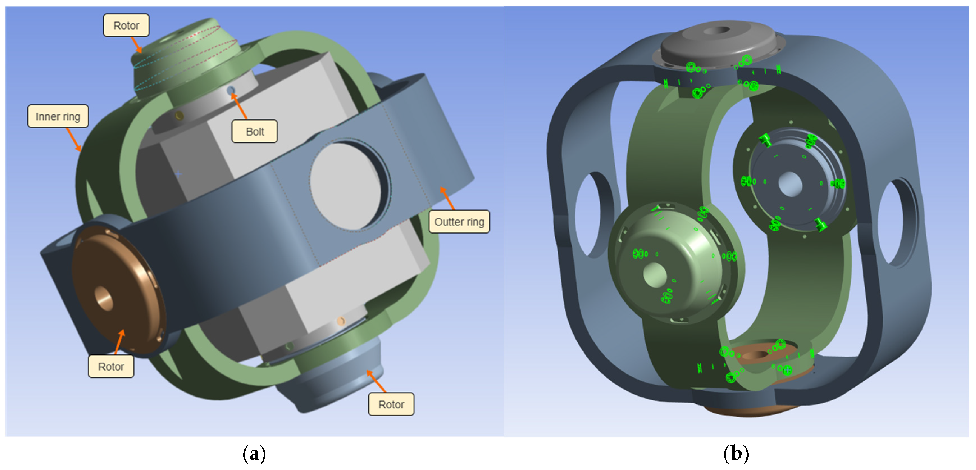
Based on these assumptions, we established a finite element model comprising the inner and outer rings, rotors, and 48 bolts (see Figure 2). The material properties were set according to the actual engineering materials, and the mesh was refined in critical areas. We used programmatic scripts to control ANSYS for batch simulations, with each data sample representing a complete assembly process. The preload vector P was sampled within the range of [3800 N, 7500 N], which was determined based on expert knowledge and torque-to-preload conversion principles. The tightening sequence vector S was generated to satisfy physical constraints described in Section 3.2. Both P and S were initialized using Latin Hypercube Sampling (LHS) to ensure sufficient coverage of the solution space. The output label for each sample is the final assembly’s orthogonal axis error, ε o r t h o , obtained from the simulation. Specifically, the two symmetric rotors on the inner ring and the outer ring each define a central axis. In an ideal state, the central axis of the inner ring and that of the outer ring should be perfectly orthogonal (at a 90° angle). However, non-uniform forces during the assembly process cause minute deviations in these axes. ε o r t h o is defined as the deviation between the actual angle of these two axes and the ideal 90°. Through this method, we generated a total of 2000 valid “assembly process–assembly error” data pairs, forming the raw dataset for this study.

3.2. Physical Constraints of the Assembly Process

The inertial gyroscope assembly studied in this paper possesses a precision structure, featuring an inner and an outer ring, each housing two rotors: one for angular velocity measurement and the other serving as a drive motor. Each rotor is secured by 6 bolts, resulting in a total of 24 critical axial bolt connections that require precise tightening. To guarantee the final performance of the gyroscope, its assembly process must adhere to a strict set of procedural specifications derived from engineering practice. The core physical objective of these specifications is to achieve a uniform stress distribution and to minimize assembly-induced structural deformations and asymmetries, which are the primary sources of orthogonal error.
These process specifications are embodied in the following four key physical constraints:
(1)
Grouped Assembly: The 24 bolts are logically divided into four groups, corresponding to the four rotors (inner ring measurement, inner ring drive, outer ring measurement, outer ring drive). During assembly, all bolts within one group must be tightened before proceeding to the next.
(2)
Fixed Inter-Group Sequence: The tightening order of the four bolt groups is strictly fixed: first the inner ring measurement rotor, followed by the inner ring drive rotor, then the outer ring measurement rotor, and finally the outer ring drive rotor. This constraint ensures consistency in the macroscopic loading process.
(3)
Symmetric Pairing: Within each 6-bolt group, the bolts are paired to form three physically symmetric pairs. Adhering to the principle of symmetry is crucial for ensuring balanced load application and counteracting bending moments.
(4)
Adjacent Tightening of Pairs: This is the most critical micro-operational constraint. Within a symmetric pair, the tightening operations for the two bolts must be consecutively adjacent. This action aims to rapidly close the local moment loop, preventing minor component warping due to one-sided forces, which is paramount for controlling the final orthogonal axis error.

3.3. Data Preprocessing and Feature Engineering

3.3.1. Feature Selection

To further refine the surrogate inputs, we excluded the initial preload variable. This decision was motivated by both expert insights and experimental evidence. According to domain experts from our collaborating research institute, the initial preload has negligible influence on the subsequent error propagation, thus adding unnecessary complexity to the surrogate. To validate this claim, we conducted a comparative analysis: when the initial preload was included, the model’s predictive accuracy degraded notably, with the R2 score dropping from 0.5353 to −0.0331. This can be explained by the fact that the initial preload is highly uncertain in practice, and including it introduces noise rather than an informative signal. Excluding this feature not only simplified the model but also improved its stability. A concise summary of this comparison is presented in Table 1. Consequently, we regenerated the dataset with only the final preload considered and excluded all features related to initial preload during feature engineering, aiming to enhance both model performance and generalization capability. Beyond simplifying the model structure, this feature selection strategy is highly practical, as it focuses on the final state of the tightening process, which is usually of key interest in engineering applications.

3.3.2. Data Transformation and Normalization

Input Features: The bolt ID (1-24) in the tightening sequence, being categorical data, is fed directly to the model as integers to be handled by an internal embedding layer. The continuous preload feature is normalized using Z-score standardization (StandardScaler) to follow a standard normal distribution with a mean of 0 and a variance of 1. This method is more robust to potential outliers compared to Min-Max scaling and is beneficial for the stable training of neural networks by centering the data.
Target Output: Considering the orthogonal axis error is a non-negative value exhibiting a right-skewed distribution close to zero, we first apply a log(1 + p) transformation to mitigate the skewness. Subsequently, we use Min-Max Normalization (MinMaxScaler) to scale the target values into the [0, 1] range. Alternative transformations (e.g., Z-score Normalization, power transformation, and Min-Max Normalization only) were evaluated during preprocessing, but log(1 + p) with Min-Max Normalization yielded the most stable and optimal performance for subsequent model training. This series of transformations not only makes the target distribution easier for the model to learn but also tries to ensure that the de-normalized output from the model cannot be a physically impossible negative value.

3.4. The Proposed AB-BiLSTM Predictive Model

In the complex assembly process, the impact of different tightening steps on the final assembly accuracy is not equal. Some key steps, such as initial diagonal tightening or final torque loading, may contain more decisive information than intermediate steps. However, standard RNNs or LSTMs may assign similar weights to all time steps when processing long sequences or “forget” the impact of early key steps due to long-distance dependency issues. To overcome this limitation, this paper designs an Attention-based Bidirectional Long Short-Term Memory (AB-BiLSTM) network. The core idea of this model is to treat the complex assembly process as a time-series problem and leverage a deep learning model to automatically capture the profound non-linear and temporal dependencies within it.
As illustrated in Figure 3, the overall architecture of the AB-BiLSTM model follows an “Encode–Attend–Decode” pattern, primarily consisting of four core modules:
(1)
Input Embedding Layer: Converts the heterogeneous input of each time step (a discrete bolt ID and a continuous preload value) into a unified high-dimensional feature vector.
(2)
BiLSTM Feature Extraction Layer: Processes the feature sequence from both forward and backward directions to capture the complete contextual information of each assembly step.
(3)
Temporal Attention Layer: Applies weights to the output of the BiLSTM layer to dynamically identify and focus on the “critical steps” that have the greatest impact on the final error.
(4)
Output Layer: Integrates the weighted information and regresses the final orthogonal axis error value.
Before detailing each module, we provide a concise summary of the model’s input–output definition in Table 2. This table explicitly defines each component’s meaning, type, dimension, and preprocessing method.
The following subsections will provide a detailed explanation of the implementation of each module:

3.4.1. Input Embedding Layer

For the input features (bolt ID and preload) at each time step, the model first maps them into a unified high-dimensional feature space via a hybrid embedding layer. The discrete bolt ID is converted into a dense vector e i d R d e using a trainable embedding layer, allowing the model to learn the underlying relationships (e.g., symmetry) between different bolts autonomously. The continuous preload value is projected into a vector e f o r c e R d e using a fully connected layer. Finally, the two vectors are concatenated to form a fused feature vector for the time step, x t = [ e i d ; e f o r c e ] R 2 d e , which serves as the input for subsequent layers.

3.4.2. BiLSTM Feature Extraction Layer

To accurately capture the complex dependency structures in the bolt tightening sequence, we employ a bidirectional LSTM (BiLSTM) network, which processes the input in both forward and backward directions. This structure enables the model to utilize full contextual information from the sequence, capturing both past and future interactions between tightening steps.
Let the embedded input at time step t be x t R d . The forward LSTM computes a hidden state h t , and the backward LSTM computes h t . The final representation for step t is the concatenation:
h t = h t ; h t R 2 d h ,
where d h is the hidden dimension of each LSTM. The entire sequence of hidden states is denoted H = h 1 , , h T R T × 2 d h .
This dual-directional representation enables the model to infer the relative importance of tightening steps not only based on their local context but also from the global sequence pattern.

3.4.3. Temporal Attention Mechanism

To differentiate the importance of various tightening steps, an attention mechanism is introduced after the BiLSTM layer. Let H = [ h 1 , h 2 , , h T ] R T × d denote the sequence of hidden states from the BiLSTM, where T is the sequence length and d is the dimensionality of each hidden state.
The attention mechanism computes a context vector c R d , representing a weighted summary of the entire sequence, as follows:
  • Each hidden state is passed through a feedforward attention network to compute an unnormalized attention score e t :
    e t = v T t a n h ( W a h t + b a ) ,
    where W a R d a × d , b a R d a , and v R d a are trainable parameters, and d a is the attention dimension.
  • The attention weights αt are obtained via a softmax over the attention scores:
    α t = e x p ( e t ) k = 1 T   e x p ( e k ) ,
  • The final context vector c is computed as the weighted sum of the hidden states:
    c = t = 1 T   α t h t ,
This context vector c encodes the dynamic contribution of each assembly step and is passed to the output layer for final error prediction.

3.4.4. Output Layer and Loss Function

Finally, the context vector c is passed through a fully connected layer to regress the final assembly error (which has been transformed and normalized). The output layer employs the Softplus activation function to ensure the model’s output is strictly non-negative.
To train the model, we designed a combined loss function to handle the small-valued, outlier-sensitive target variable. This function integrates the Mean Absolute Error (MAE) and the Log-Cosh loss [38]:
L = λ × L M A E + ( 1 λ ) × L L o g C o s h ,
The Log-Cosh loss is defined as L L o g C o s h = l o g ( c o s h ( ŷ y ) ) , where ŷ is the predicted value and y is the true value. λ is the weight between 0 and 1.
This combined loss function was carefully designed to match the prediction target of assembly error in this study. Specifically, the Log-Cosh loss offers a unique advantage: when the prediction error is small (as is the case for most instances in our task), its functional form closely approximates that of Mean Squared Error (MSE), providing a smooth, twice-differentiable surface that facilitates stable and precise fine-tuning near the optimal solution. Conversely, when the error is large, it behaves similarly to MAE, which significantly reduces the model’s sensitivity to potential outliers in the dataset, thereby enhancing its robustness. By combining Log-Cosh directly with MAE, we further amplify this robustness to outliers while maintaining a smooth gradient for optimization, making it an ideal choice for predicting small, non-negative error values.

4. Process Parameter Optimization via SEG-HHO

4.1. Mathematical Formulation of the Optimization Problem

Leveraging the trained surrogate model f A B B i L S T M ( · ) from Section 3.4, the process parameter optimization for the gyroscope assembly can be modeled as a constrained minimization problem. Our goal is to find an optimal tightening sequence S and a preload vector P that minimize the orthogonal axis error predicted by the surrogate model:
  • Decision Variables
    • The tightening sequence vector S = [ s 0 , s 1 , , s 23 ] , where s t represents the ID of the bolt being operated on at the t -th tightening step. S is a permutation of the set { 0 ,   1 ,   ,   23 } .
    • The preload vector P = [ p 1 , p 2 , , p 24 ] , where p i represents the final preload value for the bolt with ID i .
  • Objective Function
    min f A B B i L S T M ( S , P ) } .
  • Constraints
    To formally describe the assembly constraints detailed in Section 3.2, we first define the bolt groups. The 24 bolts are partitioned into four disjoint sets: G 0 = { 0 ,   ,   5 } , G 1 = { 6 ,   ,   11 } , G 2 = { 12 , , 17 } , and G 3 = { 18 ,   ,   23 } . The decision variables must satisfy the following conditions:
    • p i P m i n , P m a x , for all i { 0 , , 23 } .
    • must satisfy the four process constraints of grouping, group order, symmetry, and adjacency as defined in Section 3.2.
This mathematical model clearly defines the optimization task. However, because the decision variable S is a discrete permutation subject to complex combinatorial constraints, traditional methods like gradient-based optimization methods are not directly applicable. Therefore, we employ a metaheuristic algorithm and handle these constraints using a specialized encoding–decoding mechanism, which will be introduced in Section 4.2 and Section 4.3.

4.2. The Improved Harris Hawks Optimization Algorithm, SEG-HHO

4.2.1. Standard HHO

The Harris Hawks Optimization (HHO) algorithm is a metaheuristic algorithm that mimics the cooperative predatory behavior of Harris’s hawks. Its core lies in simulating the strategies of exploration and exploitation that the hawk flock employs at different stages to capture prey (the optimal solution). A key parameter in the optimization process is the prey’s escaping energy, E , which decreases from 2 to 0 as the number of iterations t increases. Its formula is:
E = 2 E 0 1 t T m a x ,
where T m a x is the maximum number of iterations, and E 0 is a random initial energy varying within ( 1 ,   1 ) . The HHO process primarily consists of two phases:
  • Exploration Phase ( | E | 1 ): In this phase, the hawks widely search for prey, updating their position X ( t + 1 ) using one of two strategies based on a random number q :
    X ( t + 1 ) = X r a n d t r 1 X r a n d t 2 r 2 X t ,     q < 0.5 X ( t + 1 ) = X r a b b i t t X m t r 3 l b + r 4 u b l b ,     q 0.5 ,
    where X r a b b i t is the current best solution (prey’s location), X r a n d is a randomly selected hawk, X m is the average position of the population, and r 1 to r 4 are random numbers in ( 0,1 ) ; l b and u b , respectively, represent the lower and upper bounds of the search space.
  • Exploitation Phase ( | E | < 1 ): The hawks besiege the discovered prey. This phase simulates four different attack behaviors based on the energy | E | and the escape probability r :
  • Soft Besiege: When r 0.5 and | E | 0.5 , the hawks gradually encircle the prey.
    X ( t + 1 ) = Δ X ( t ) E | J X r a b b i t ( t ) X ( t ) | ,
    where Δ X ( t ) = X r a b b i t ( t ) X ( t ) represents the positional difference between the current individual and the prey. J = 2 ( 1 r 5 ) represents the random jumping intensity of prey during escape, and r 5 is a random number in ( 0 ,   1 ) .
  • Hard Besiege: When r 0.5 and | E | < 0.5 , the prey is exhausted, and the hawks tighten their encirclement.
    X ( t + 1 ) = X r a b b i t ( t ) E | Δ X ( t ) | ,
  • Soft Besiege with Progressive Rapid Dives: When r < 0.5 and | E | 0.5 , the prey attempts an erratic escape, and the hawks employ dive strategies based on Levy Flight (LF).
    X ( t + 1 ) = Y , f ( Y ) < f ( X ( t ) ) Z , f ( Z ) < f ( X ( t ) ) ,
    Y = X r a b b i t ( t ) E | J X r a b b i t ( t ) X ( t ) | ,
    Z = Y + S × L F ( D ) ,
    L F x = 0.01 × u × σ | v | 1 β ,
    σ = Γ ( 1 + β ) × s i n ( π β 2 ) Γ ( 1 + β 2 ) × β × 2 ( β 1 2 ) 1 β ,
    where f · represents the individual’s fitness value; D is the dimension of the problem; S is a 1 × D random vector; u , v are random numbers within (0,1); β is usually set to 1.5; and Γ   is a standard gamma function with the following expression: Γ ( x ) = 0 +   e t t x 1 d t .
  • Hard Besiege with Progressive Rapid Dives: When r < 0.5 and | E | < 0.5 , the hawks launch a final assault, incorporating Levy Flight in the final encirclement:
    X ( t + 1 ) = Y , f ( Y ) < f ( X ( t ) ) Z , f ( Z ) < f ( X ( t ) ) ,
    Y = X r a b b i t ( t ) E J X r a b b i t t X m t ,
    Z = Y + S × L F ( D ) ,

4.2.2. The Proposed Stratified and Hybrid Search Strategies

To overcome the limitations of the standard HHO, such as its tendency to fall into local optima and its insufficient exploration capability when dealing with complex optimization problems, this paper introduces a series of improvements in three key areas: population initialization, population structure, and search strategy, forming the Stratified Evolutionary and Hybrid search-based SEG-HHO algorithm.
Initialization via Tent Chaotic Map. Unlike the standard random initialization of HHO, our algorithm employs a Tent chaotic map to generate the initial population. In contrast to standard random initialization, which can lead to population clustering, the ergodic and non-repetitive properties of chaotic systems allow the initial population to be more uniformly distributed throughout the search space, thereby enhancing the algorithm’s global search efficiency. The mathematical definition of the Tent map is as follows:
z t + 1 = z t μ ,     0 < z t μ 1 z t 1 μ ,     μ < z t < 1 ,
where z t ( 0,1 ) is the chaotic variable at iteration t , and μ ( 0,1 ) is the control parameter, typically set to μ = 0.5 for standard Tent behavior
We first randomly generate an initial chaotic vector z 0 and then iterate the map N times (with N being the population size) to produce a set of chaotic values z 1 , z 2 , , z N . Finally, these values are mapped to the problem’s search space [ X m i n , X m a x ] to generate the initial population’s position vectors X (each individual has D dimensions) using the following equation:
X i , j = X m i n ( j ) + z i , j × X m a x j X m i n j , i = 1 , , N ; j = 1 , , D ,
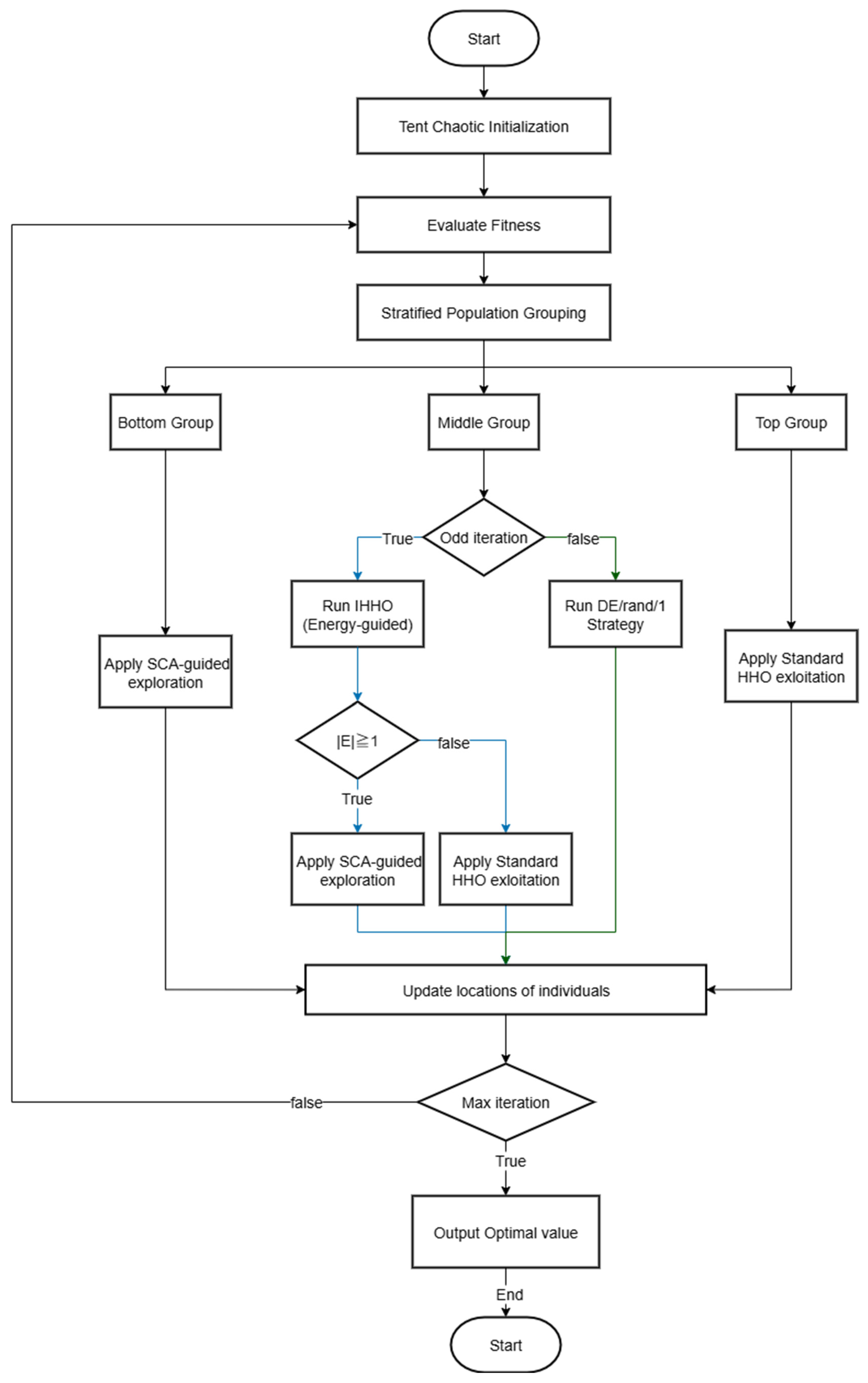
Stratified Evolutionary Framework. Building on this, we introduce the concept of stratified evolution, where the population is dynamically divided into three functionally distinct sub-populations in each generation based on individual fitness values: the top group (top 1/3, responsible for deep exploitation), the middle group (middle 1/3, responsible for adaptive hybrid strategy), and the bottom group (bottom 1/3, responsible for broad exploration). This structured population makes it possible to design targeted search strategies for sub-populations with different characteristics.
Hybrid Search Mechanisms for Different Evolutionary Groups. To achieve efficient global optimization, each sub-population is assigned a unique update strategy designed to overcome specific deficiencies of the standard HHO:
  • Bottom Group: Incorporating SCA for Structured Exploration. The exploration mechanism of standard HHO relies on random walks, which can sometimes result in inefficient search paths. To address this, we integrate the core principles of the Sine Cosine Algorithm (SCA) to guide the bottom group. SCA leverages the smooth, periodic oscillations of sine and cosine functions, enabling exploratory individuals to probe the space around the current best solution in a wave-like, more directional manner. Its position is updated as follows:
    When q < 0.5 ,
    X t + 1 = X t + R 1 × s i n R 2 × R 3 X r a n d t X t ,     R 4 < 0.5 X t + 1 = X t + R 1 × c o s R 2 × R 3 X r a n d t X t ,     R 4 0.5 ,
    where R 1 is a control parameter that linearly decreases from 2 to 0 to balance exploration and exploitation; R 2 ,   R 3 , and R 4 are random control parameters for SCA in the ranges [ 0 ,   2 π ] , [ 0 ,   2 ] , and [ 0 ,   1 ] respectively. This structured exploration, compared to purely random jumps, more effectively covers promising regions.
  • Middle Group: Alternating Hybrid Search with HHO and Differential Evolution (DE). To improve exploration–exploitation balance and enhance population diversity, the middle group adopts an alternating hybrid strategy based on iteration count. Specifically, the algorithm executes HHO during odd-numbered iterations and a DE scheme during even-numbered iterations.
    In the HHO phase (odd iterations), the algorithm determines its behavior based on the prey’s escaping energy. When the energy is high, the algorithm performs exploration using enhanced strategies inspired by SCA, which enables the search agents to traverse the space more dynamically. When the energy is low, the algorithm switches to the four classical exploitation strategies of HHO, allowing the population to rapidly converge toward the current best solution.
    In the DE phase (even iterations), the algorithm introduces the “DE/rand/1” mutation and binomial crossover to inject diversity and prevent premature convergence. For each target vector X i , a mutant vector V i is generated using:
    V i ( t ) = X r 1 ( t ) + F m u t × ( X r 2 t X r 3 ( t ) ) ,
    where r 1 , r 2 , and r 3 are distinct random indices from the population and F m u t is the mutation scaling factor. This is followed by binomial crossover to produce the trial vector U i .
    DE generates new individuals based on the difference vectors between existing population members, which is an extremely effective mechanism for maintaining diversity. By introducing this “perturbation,” we significantly enhance the algorithm’s ability to escape local optima in complex multimodal problems.
  • Top Group: Intensifying Local Exploitation to Accelerate Convergence. For the top group, which consists of the fittest individuals, the primary mission is the rapid and precise excavation of promising regions already discovered. Therefore, we retain and intensify the highly efficient hard and soft besiege strategies from the standard HHO. This ensures that the algorithm can leverage the collective intelligence of the population in its final stages to perform a swift refinement of the optimal solution, thereby guaranteeing final convergence accuracy.
The complete process of the proposed SEG-HHO algorithm is summarized in Algorithm 1. The flowchart of SEG-HHO is shown as Figure 4.
Algorithm 1 The Proposed SEG-HHO Algorithm
Input:
N : Population size
D : Problem dimension
T m a x : Maximum number of iterations
F m u t , C r : Parameters for Differential Evolution
L B , U B : Lower and upper bounds of the search space
Output:
X b e s t : The best solution found
f ( X b e s t ) : The fitness of the best solution

1 :   Initialize   population   X = { X 1 , X 2 , , X N } using the Tent chaotic map.
2 :   Evaluate   the   fitness   f X i   for   each   individual   X i .
3 :   Identify   the   initial   global   best   solution   X b e s t .
4:
5 :   for   t = 1   to   T m a x  do
6 :        Sort   the   population   X by fitness in ascending order.
7 :        Partition   X into three groups:
8 :            X t o p   Top   N / 3   individuals   ( indices   1   to   N / 3 ).
9 :            X m i d   Middle   N / 3   individuals   ( indices   N / 3 + 1   to   2 N / 3 ).
10 :            X b t m   Bottom   N / 3   individuals   ( indices   2 N / 3 + 1   to   N ).
11:
12:      // Process the Top Group: Intensive Exploitation
13 :        for   each   individual   X i   in   X t o p  do
14 :            X i   Apply _ HHO _ Exploitation _ Phase X i , X b e s t
15:      end for
16:
17:      // Process the Bottom Group: SCA-Enhanced Exploration
18 :   for   each   individual   X i   in   X b t m  do
19:          // This group exclusively uses the HHO exploration logic
20 :            X i   Apply _ SCA _ Enhanced _ Exploration _ Phase ( X i )
21:      end for
22:
23:      // Process the Middle Group: Alternating Hybrid Search
24 :        if   mod ( t ,   2 )   0 then // Odd Iteration
25 :            for   each   individual   X i   in   X m i d  do
26 :                X i   Apply _ Full _ HHO _ Operator ( X i ,   X b e s t ) // Includes both SCA_Enhanced_Exploration and exploitation
27:          end for
28:      else // Even Iteration
29 :            for   each   individual   X i   in   X m i d  do
30 :                X i   Apply _ DE _ Operator ( X i ,   X i n t e r ) // DE operates within its own subgroup
31:          end for
32:      end if
33:
34:      // Combine, Evaluate, and Update Global Best
35 :        Combine   all   updated   individuals   from   the   three   groups   into   the   main   population   X .
36:      Evaluate the fitness of any newly generated individuals.
37 :        Update   X b e s t   if   a   better   solution   is   found   in   the   current   population   X .
38: end for
39:
40 :   Return   X b e s t
To further clarify the roles of each sub-population and the novelty of our proposed hybrid strategy, Table 3 provides an intuitive summary of the SEG-HHO phases, and Table 4 offers a detailed comparison between SEG-HHO and its foundational algorithms.
As shown in Table 3, the core novelty of SEG-HHO is not merely the inclusion of DE and SCA operators but the creation of a systematic, role-based population structure. Unlike many hybrid algorithms that apply the same logic to all individuals, SEG-HHO assigns specific, complementary tasks to different population segments, creating a more organized and efficient search dynamic. Table 4 further contrasts SEG-HHO with its component algorithms, highlighting its unique synthesis.

4.3. Encoding and Decoding Mechanism for Assembly Constraints

To employ the continuous variable-based SEG-HHO algorithm for solving the mixed-variable optimization problem, which involves continuous preload variables and discrete tightening sequence variables, an effective encoding and decoding scheme is imperative. This scheme is designed to map a complex solution that adheres to the assembly process constraints (as detailed in Section 3.2) into a standardized real-valued vector, thereby building a bridge from the algorithm’s search space to the physically feasible solution space.

4.3.1. Definition of the Hybrid Encoding Vector

We encode each candidate solution into a 48-dimensional real-valued vector X R 48 . This vector is composed of three concatenated parts:
X = [ P ; K ; Δ ] ,
where:
P = [ p 0 , p 1 , , p 23 ] is a 24-dimensional vector directly representing the preload values of the 24 bolts. Each element p i is constrained within a predefined physical boundary [ P m i n ,   P m a x ] .
K = [ k 0 ,   k 2 ,   ,   k 11 ] is a 12-dimensional vector used to encode the relative tightening order of the three symmetric bolt pairs within each of the four bolt groups.
Δ = [ δ 0 ,   δ 1 ,   ,   δ 11 ] is a 12-dimensional vector used to encode the internal tightening direction (i.e., which bolt is tightened first) for each of the 12 symmetric pairs.
Each element within the K and Δ vectors is bounded in the range 0 ,   1 .

4.3.2. The Decoding Process

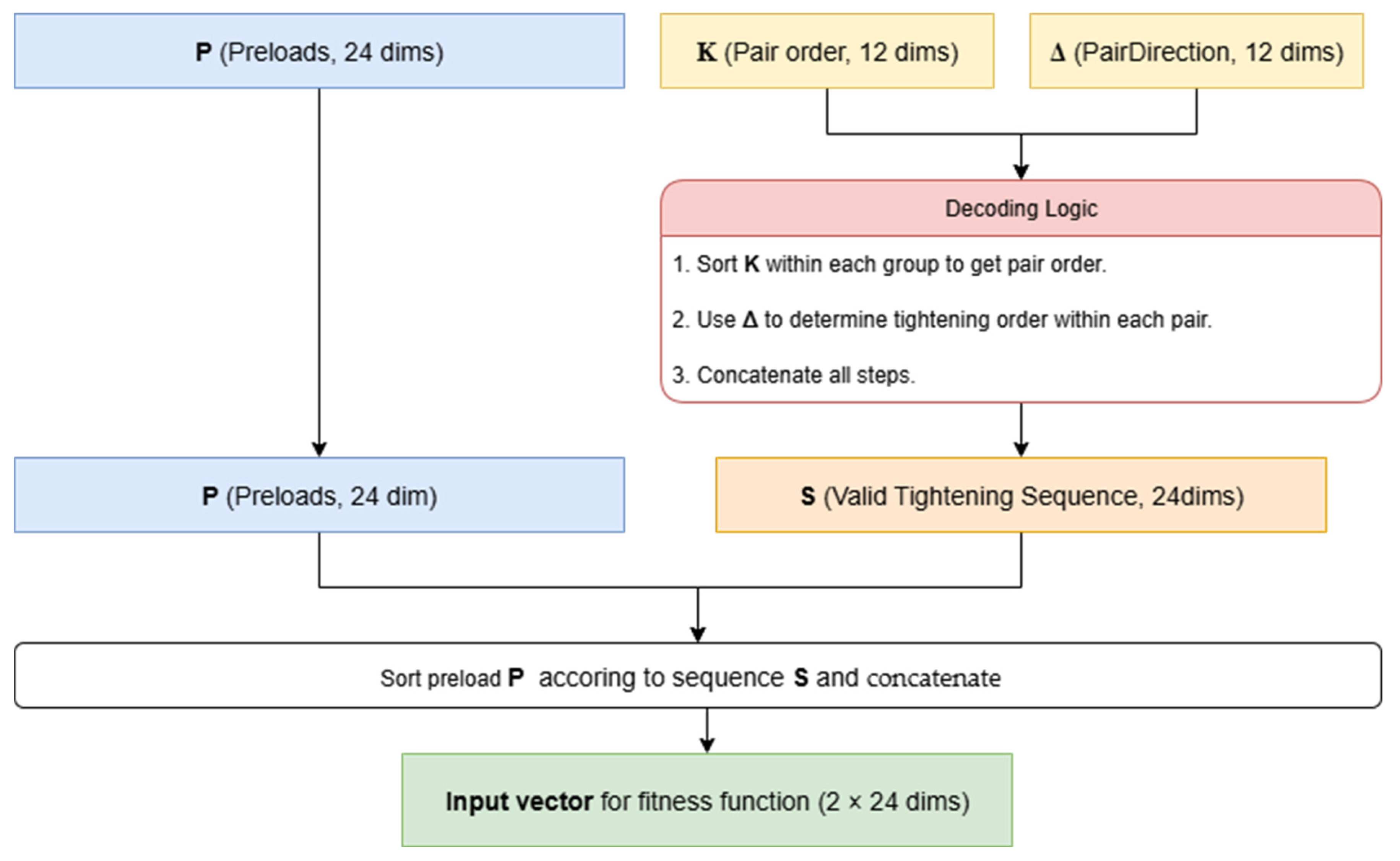
Decoding is the process of converting an arbitrary 48-dimensional vector X , generated by the optimization algorithm, into a unique and physically valid tightening sequence S and a preload vector P .
  • Preload Decoding: The vector P requires no further decoding; its 24 elements directly correspond to the final preload values for the 24 bolts.
  • Tightening Sequence Decoding: The generation of the tightening sequence S adheres to the predefined assembly constraints and is achieved through a programmatic decoding of the K and Δ vectors. The decoding algorithm proceeds according to the fixed group order ( G 0 G 1 G 2 G 3 ), with the following steps:
    • For the g -th bolt group ( g { 0 , 1 , 2 , 3 } ), its corresponding sequence-encoding sub-vector K g = k 3 g , k 3 g + 1 , k 3 g + 2 and direction-encoding sub-vector Δ g = δ 3 g , δ 3 g + 1 , δ 3 g + 2 are extracted.
    • The a r g s o r t operation is applied to K g to determine the tightening order index O r d e r p a i r for the three symmetric pairs within the group.
    • The three pairs are processed sequentially according to O r d e r p a i r . For the j -th symmetric pair { A , B } , its corresponding direction-encoding value δ g , j is queried. If δ g j < 0.5 , the tightening order is A B ; otherwise, it is B A .
    • After executing the decoding for all four groups, a final tightening sequence vector S of length 24, which fully satisfies all adjacency and symmetry constraints, is concatenated.
Through this encoding–decoding mechanism, every candidate solution generated in each iteration of the optimization algorithm can be deterministically mapped to a valid assembly process scheme. Its performance is then rapidly evaluated by the AB-BiLSTM surrogate model described in Section 3.4.
The encoding and decoding mechanisms are shown as Figure 5 and Figure 6. Figure 5 provides a conceptual and schematic overview of the encoding–decoding mechanism. This diagram illustrates the mapping from the 48-dimensional continuous vector X , optimized by SEG-HHO, to the final physically constrained assembly plan, consisting of a discrete tightening sequence S and a continuous preload vector P . The decoding logic ensures all assembly rules (grouping, symmetry, and adjacency) are inherently satisfied. Figure 6 illustrates the decoding process with a concrete numerical example.

4.3.3. Discussion on the Constraint-Handling Strategy

The encoding–decoding mechanism employed in this study is a constructive approach to constraint handling. Its primary advantage lies in the deterministic decoding process, which guarantees that any candidate solution vector X generated by the optimization algorithm in the continuous search space is uniquely mapped to a feasible assembly scheme that is 100% compliant with all physical constraints (e.g., grouping, symmetry, and adjacency). This “feasible-by-design” paradigm precludes the generation of any physically infeasible solutions during the optimization process.
To better contextualize our choice of strategy, it is useful to compare it with two other widely used constraint-handling techniques:
Penalty Functions: This method allows the algorithm to generate infeasible solutions but discourages them by adding a large penalty term to the fitness function. While simple to implement, its performance is highly sensitive to the penalty coefficient, which, if too small, fails to effectively exclude infeasible solutions, and if too large, can distort the fitness landscape and mislead the search.
Repair Operators: This approach programmatically modifies an infeasible solution to make it feasible before evaluation. While it avoids parameter tuning, designing an efficient repair operator that does not disrupt the beneficial schemata within a solution is challenging and may introduce additional computational overhead.
Given the highly coupled and strict nature of the assembly constraints in this task, we selected the constructive encoding–decoding approach. This method ensures that the surrogate model is always evaluated on physically meaningful, feasible inputs, which preserves the smoothness of the fitness landscape and eliminates the complexity of tuning penalty or repair parameters. Although the initial design of the decoder is more complex, it establishes a solid foundation for efficient and reliable optimization.

5. Experiments and Result Analysis

5.1. Experimental Setup

5.1.1. Dataset Overview and Partitioning

The machine learning experiments in this study are based on the dataset of 2000 samples generated via FEM simulation, as described in Section 3.1. To reliably evaluate model performance, we strictly partitioned the dataset into a training set, a validation set, and a test set, with a ratio of 60%:20%:20%. Model training was conducted on the training set, hyperparameter tuning was based on performance on the validation set, and the final model evaluation was performed on the independent test set, which the model had never seen before.

5.1.2. Experimental Environment

To ensure computational efficiency and software compatibility, the simulations and model training tasks were executed on the same physical server but under different operating systems. Specifically, the finite element simulations were performed under Windows 10 Pro using ANSYS 2023R1 software, while the training and validation of deep learning models were conducted under Ubuntu 22.04 LTS, optimized for GPU-based computing and open-source frameworks. The server is equipped with two physical Intel Xeon Silver 4310 CPUs, an NVIDIA RTX A6000 GPU (48 GB VRAM), and 128 GB RAM, supporting a dual-boot configuration.
The benchmark performance tests on the CEC2005 functions were carried out on a local PC (CPU: Intel i5-12400F, RAM: 16 GB, OS: Windows 10) using MATLAB R2021a to run the official benchmark suite.
All other algorithm components, including model inference and assembly optimization, were implemented in Python 3.11, using open-source libraries such as PyTorch-Lightning 2.5.0, NumPy 2.3.2, and SciPy 1.16.0.

5.1.3. Performance Metrics

To comprehensively evaluate the performance of both the predictive models and the optimization algorithms, we adopted a set of metrics tailored to each task category.
Predictive Model Performance Metrics: The accuracy of the AB-BiLSTM prediction model was assessed using three standard regression metrics: Root Mean Squared Error (RMSE), MSE, MAE, and the Coefficient of Determination ( R 2 ). Given a ground truth vector y , a predicted vector y ^ , and the mean of the true values y ¯ , their definitions are as follows:
R M S E = 1 n i = 1 n y i y ^ i 2 ,
M S E = 1 n i = 1 n y i y ^ i 2 ,
M A E = 1 n i = 1 n y i y ^ i ,
R 2 = 1 i = 1 n y i y ^ i 2 i = 1 n y i y ¯ i 2 ,
These metrics collectively reflect the model’s prediction accuracy, stability, and fitting quality.
Optimization Algorithm Benchmark Metrics: For benchmarking the optimization algorithms on the CEC2005 test suite, we employed classical numerical indicators, including the best, mean, worst, and standard deviation of objective values across 30 independent runs. To further assess statistical significance and overall performance ranking, we applied the Friedman test, a non-parametric method that ranks algorithms across all benchmark functions and computes an average rank score. This metric provides a fair and comparative view of algorithm robustness and consistency across different problem types.

5.2. Performance Evaluation of Predictive Models

5.2.1. Model Selection

To ensure that the proposed AB-BiLSTM model achieves its optimal performance and to establish a fair platform for subsequent baseline comparisons, we first conducted a systematic search and optimization for the model’s key hyperparameters. We employed the Optuna framework, a state-of-the-art automated hyperparameter search tool that uses the Tree-structured Parzen Estimator (TPE) algorithm to execute Bayesian optimization. The optimization objective was set to minimize the combined loss on the validation set through 150 trials. The search space for the key hyperparameters is detailed in Table 5.
After the optimization process, the resulting optimal hyperparameter combination is presented in Table 6. To maintain fairness in the following comparative experiments, all sequence-based models (e.g., RNN, LSTM, GRU, and BiLSTM) uniformly adopted the same key architectural parameters, such as the number of layers and hidden dimensions.
To comprehensively evaluate the performance of the proposed model, we selected several classic machine learning and deep learning models as benchmarks. The architectural parameters for all comparative models are configured as shown in Table 6 to ensure the rigor of the comparison. For non-sequential baseline models (MLP and 1D-CNN), standard architectures were adopted with commonly used activation functions (e.g., ReLU). The layer dimensions of these models were configured to match the hidden layer dimension of the sequence models, enabling a fair structural comparison. The detailed architectures for all comparative models are shown in Table 7.

5.2.2. Experiment Results

In this section, we present a comprehensive performance comparison of the proposed AB-BiLSTM model against several benchmarks and provide an in-depth analysis of its training process and prediction efficiency.
First, we examined the training convergence of the AB-BiLSTM model. As shown in Figure 7, both the training loss and validation loss decrease steadily with the number of epochs and eventually converge to a low level. The absence of a significant gap between the two curves indicates that the model learned effectively without suffering from severe overfitting, thus validating its good generalization ability.
Table 8 summarizes the comprehensive performance metrics of all models on the test set. It is evident from this table that the proposed AB-BiLSTM model significantly outperforms all other baseline models across all key evaluation metrics. Specifically, the AB-BiLSTM achieved an MAE of 3.5949E−05 and an RMSE of 5.3333E−05, both of which are the lowest among all models, indicating the smallest average deviation between its predictions and the true values. Its R2 score reached an impressive 0.8173, surpassing the sub-optimal LSTM model (R2 = 0.8077) and BiLSTM model (R2 = 0.8017). All these performances strongly demonstrate that the introduction of the temporal attention mechanism effectively enhances the model’s ability to capture critical information within the assembly process, leading to more accurate error prediction.
We further investigated the model’s prediction behavior in the region of extremely small target values. Figure 8 illustrates the trend of the R2 score as the true error value changes. It can be observed that as the true error value approaches zero, the R2 metric becomes extremely sensitive and exhibits a non-linear decline, even yielding negative values. This is not indicative of model failure but is an inherent characteristic of the R2 metric itself, where any minute prediction deviation from a near-zero baseline can result in an R2 score far less than 1. This analysis confirms the rationality and foresight of our choice to use MAE as a core evaluation metric and to design a combined loss function.
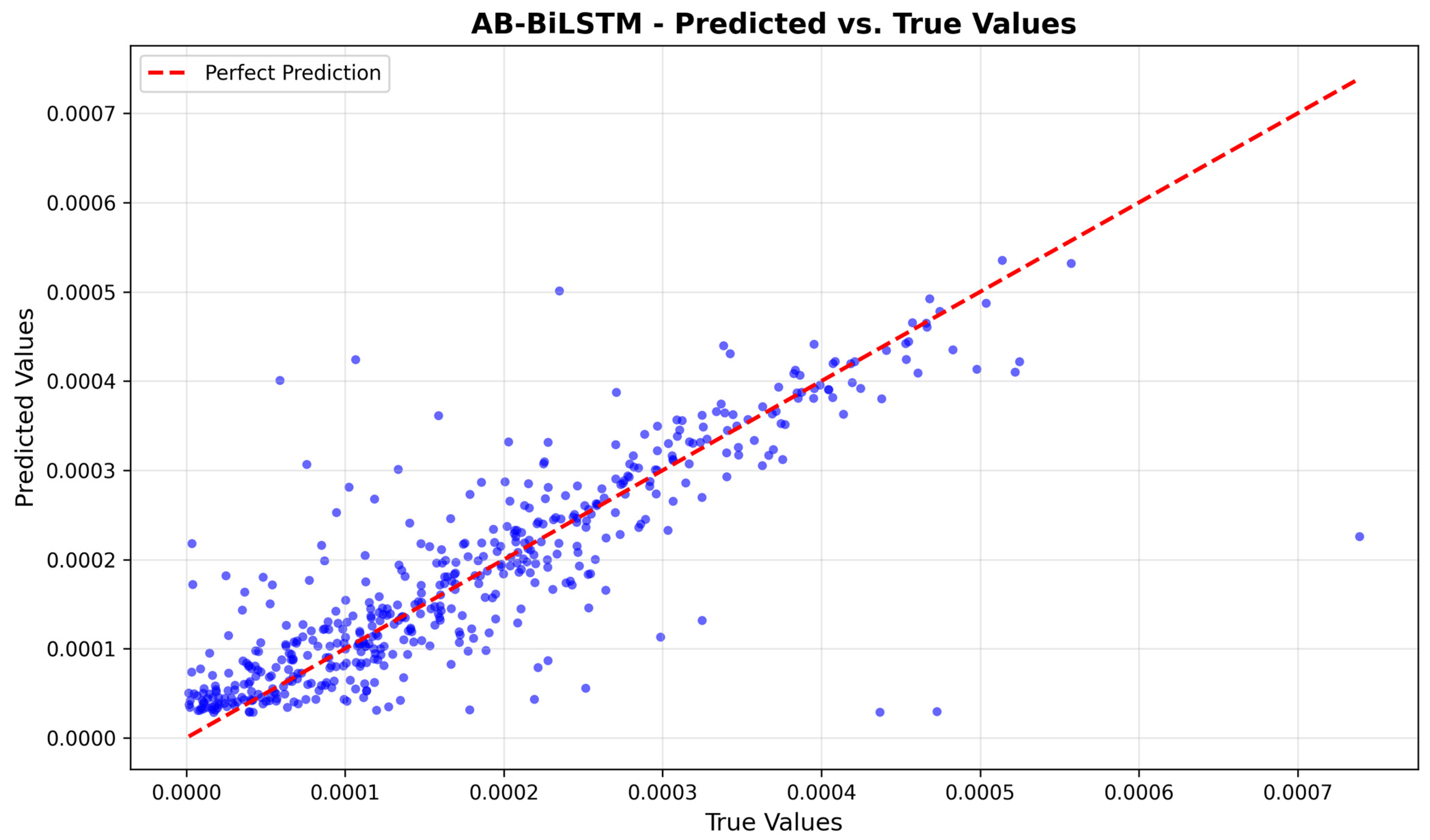
To provide a more granular view of the model’s prediction performance, we have included additional error analyses in the appendix. Appendix A.1 presents a scatter plot of the predicted versus actual orthogonal axis errors on the test set, which visually demonstrates the high correlation between the model’s predictions and the ground truth values. Furthermore, Appendix A.2 contains a histogram of prediction errors, illustrating that the errors are tightly centered around zero with a quasi-normal distribution, confirming the absence of systematic bias in our model.
When evaluating computational efficiency, we also compared the training time and single-prediction latency of each model in Table 3. All deep learning-based surrogate models can complete a prediction at the millisecond level, whereas a traditional FEM simulation requires approximately 14 min for a single run. Taking our proposed AB-BiLSTM model as an example, its single-prediction latency is merely 1.1753 ms. By calculation, this yields a speed-up ratio of approximately 714,711, representing an efficiency improvement of several orders of magnitude over FEM. The comparison results are shown in Table 9.
In summary, although the AB-BiLSTM exhibits a slightly longer training time (189.8061 s) and prediction latency (1.175323 ms) due to its more complex architecture, it achieves a decisive advantage in prediction accuracy. This characteristic—trading a marginal cost in efficiency for a substantial gain in precision—highlights the immense potential and practical value of the proposed framework for engineering applications that require rapid design optimization and iteration.

5.2.3. Analysis of the Attention Mechanism

To dissect and validate the pivotal role of the attention mechanism within the AB-BiLSTM model, a comprehensive evaluation involving an ablation study and visualization analysis was performed.
Ablation Study: First, the contribution of the attention mechanism was quantified by comparing the performance of the AB-BiLSTM model against a standard BiLSTM model from which the attention module was removed, as shown in Table 10. The results indicate that the AB-BiLSTM achieved a 3.92% relative improvement in MAE, while reducing MSE, RMSE, and R2 score by 8.54%, 4.18%, and 1.95%, respectively. This significant performance gain confirms that the introduction of the attention mechanism is a key factor in the model’s superior predictive accuracy.
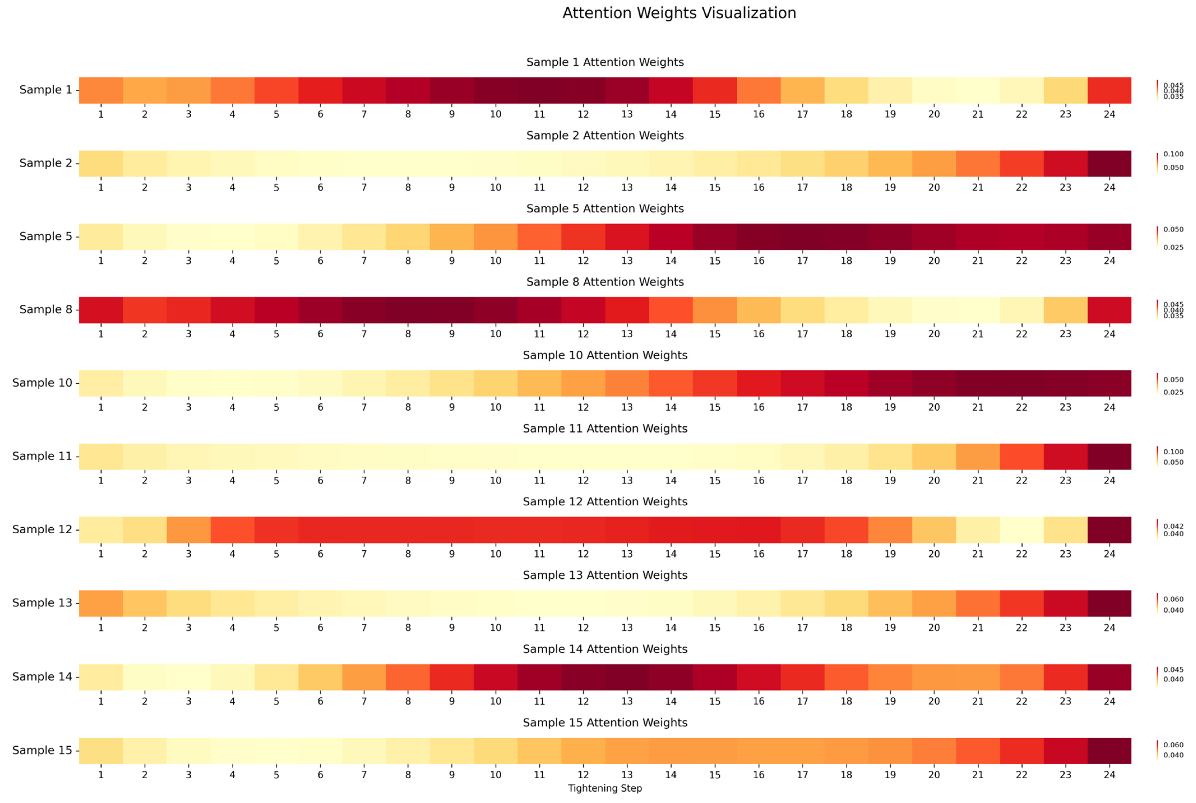
Attention Weight Visualization and Pattern Analysis: Second, to investigate how the model leverages the attention mechanism to learn physically meaningful patterns, we visualized the attention weight distributions for multiple test samples, as shown in Figure 9 (attention_visualization.jpg).
  • Global Pattern: A Focus on the “Bookends” of the Process. We first visualized the attention weight heatmaps for ten representative test samples, as shown in Figure 9 (attention_visualization.jpg). The results reveal a consistent global pattern: firstly, the attention weights are significantly concentrated in the final stage of the assembly process (steps 19–24) across most samples (7 of 10), with the final step (step 24) always receiving one of the highest weights across all samples. Secondly, the first step in many samples also receives relatively high attention in early steps, forming a “bookend” pattern of focus. This pattern is highly interpretable from a physical standpoint: the first step establishes the initial baseline for the entire process, while the final few steps “lock in” the ultimate stress state and micro-deformations, making both ends critically influential on the final error.
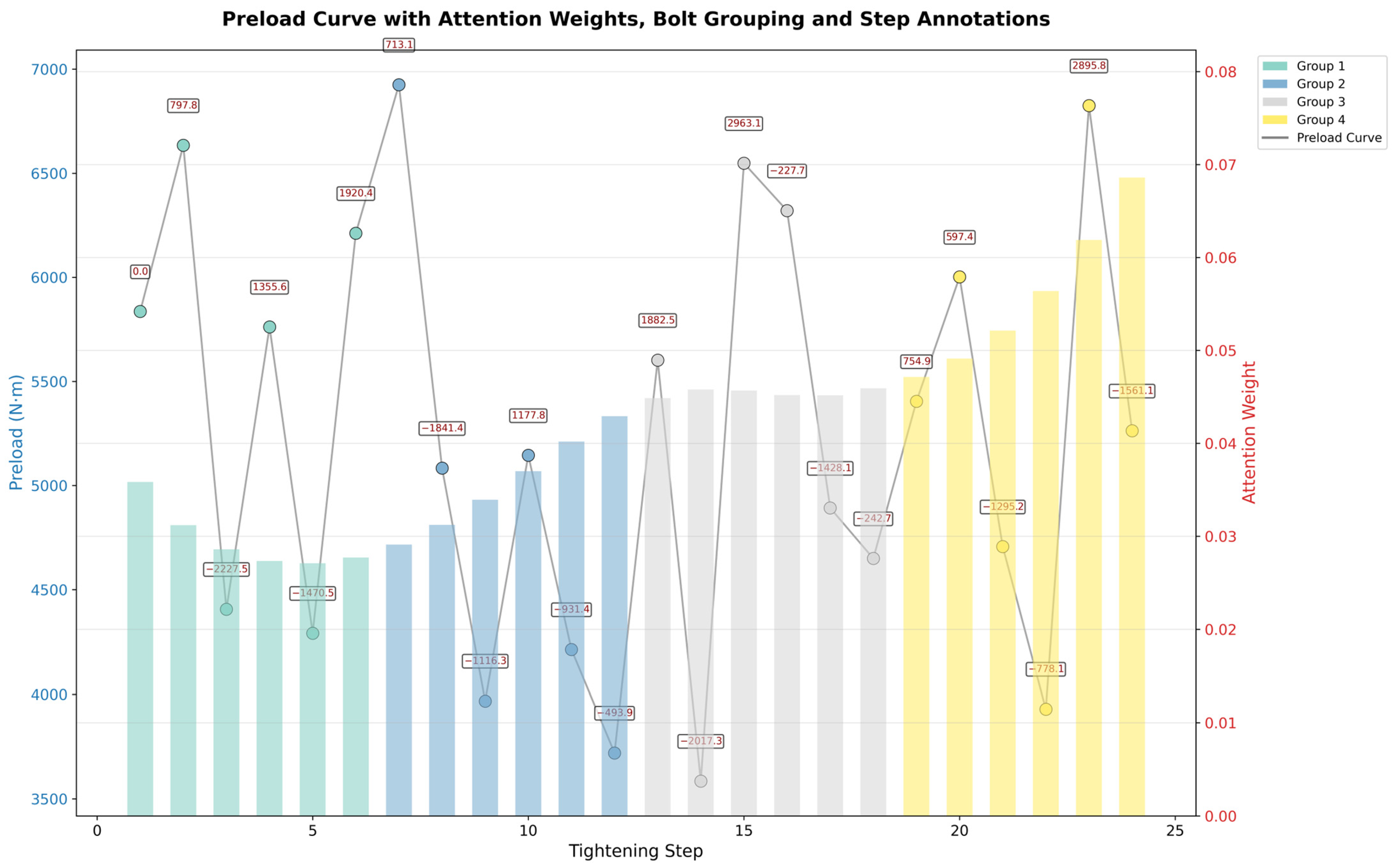
  • Local Pattern: The Non-linear Nature of Attention Allocation. To further investigate the details, we performed a case study on a representative sample (corresponding to Sample 15 in Figure 9), overlaying the preload curve, preload changes (ΔPreload), and attention weights, as shown in Figure 10.
It is visually apparent that the fluctuations in attention weights (bar chart) do not directly correspond to the magnitude of the ΔPreload values (numbers above the curve). To quantitatively verify this observation, we conducted a Pearson correlation analysis between ΔPreload and the change in attention weights (ΔAttention) for this sample, as depicted in Figure 11. The result confirms a near-zero linear correlation (r = −0.0251, p = 0.907), providing strong evidence that the model’s attention allocation is not a simple reaction to drastic changes in force but rather a more complex, non-linear decision process contingent on global context and step position.
3.
Structural Knowledge Learning: Capturing the “Rhythm” of Assembly. Given that attention is not merely a response to force values, we hypothesized that it might have learned the inherent structural knowledge of the assembly process, particularly the grouping of bolts. To test this, we statistically analyzed the absolute change in attention (|ΔAttention|) across all test samples, comparing the changes that occur within a bolt group to those at the transition between groups. The box plot in Figure 12 reveals a profound finding: the variance of |ΔAttention| is significantly lower when switching between groups (right box in Figure 12) compared to the changes within a group (left box in Figure 12).
This indicates that the model has learned a generalizable and standardized “group-tightening” template or meta-strategy. The smooth transition in attention at group switches suggests the model perceives the process for different component groups as highly consistent. The greater variance within a group implies that the model’s more fine-grained decision-making is focused on assessing the relative importance of the steps inside a single component’s assembly. This discovery confirms that the attention mechanism has learned not only “which steps are important” but, on a deeper level, the very “rhythm” and “modularity” of the assembly task.

5.2.4. Anti-Noise Robustness Test

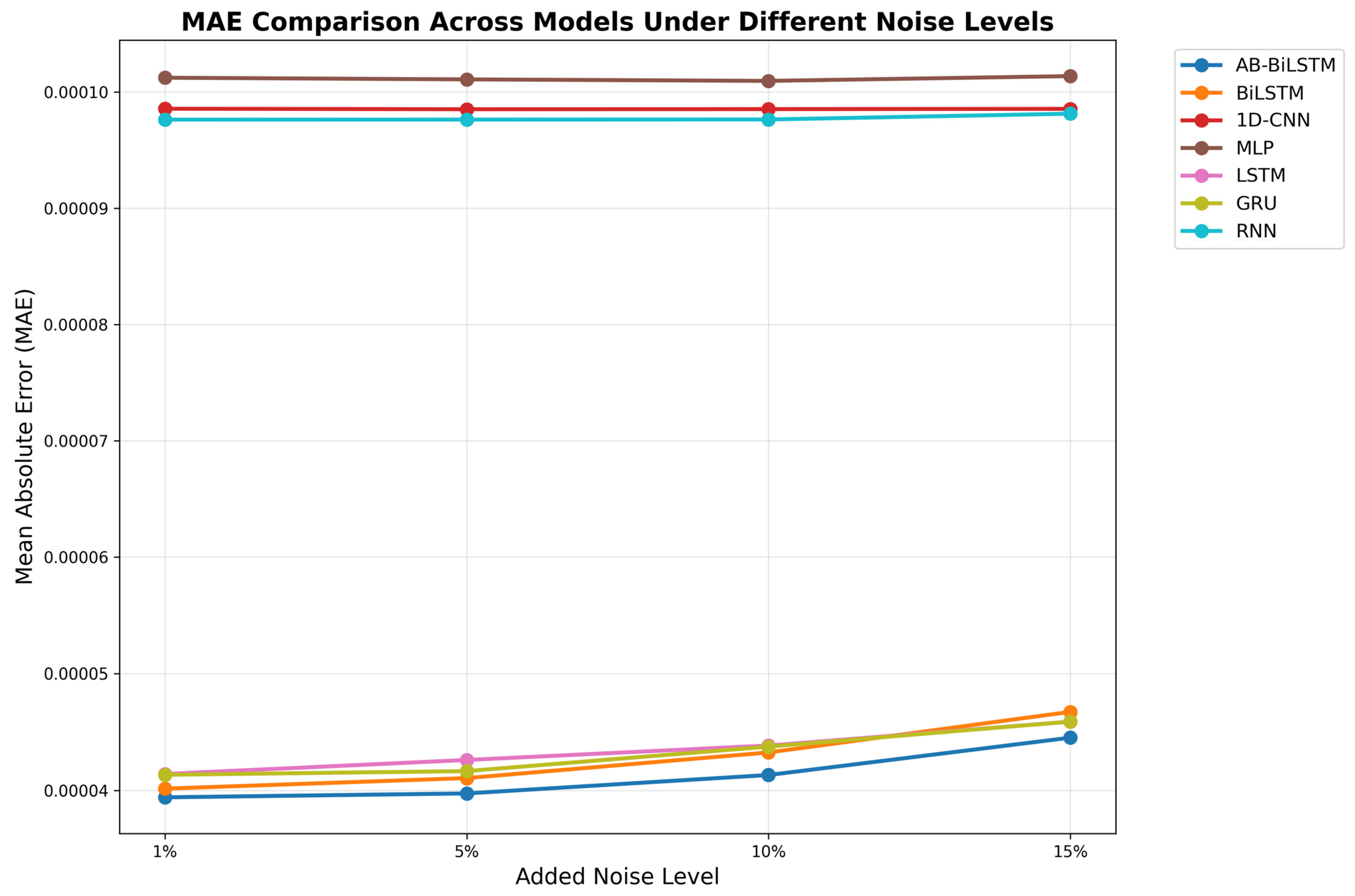
To evaluate the robustness of the proposed method under noisy input conditions, which simulates the sensor measurement errors common in industrial assembly lines, we conducted a systematic anti-noise test. Gaussian noise was injected into the normalized preload features at four intensity levels: 1%, 5%, 10%, and 15%, relative to the feature’s standard deviation.
As illustrated in Figure 13 and detailed in Table 11, the models exhibited two distinct response patterns to the introduced noise. The first group, comprising all sequence-aware models (AB-BiLSTM, BiLSTM, LSTM, GRU, and RNN), demonstrated superior resilience. These models started with a low Mean Absolute Error (MAE) baseline (approximately 4.0e−5 in 1% noise) and showed only a graceful, gradual degradation in performance as noise levels increased. For instance, our proposed AB-BiLSTM model, which had the lowest MAE across all noise levels, saw its MAE only rise from 3.91 × 10⁻⁵ to 4.45 × 10⁻⁵ when the noise level increased from 1% to 15%. This confirms its stable predictive capability in potentially noisy environments. Conversely, the second group of non-sequential models (MLP and 1D-CNN) had a much higher initial MAE (approximately 1.0e−4) and showed relative insensitivity to increasing noise. This suggests their failure to learn the underlying physical patterns from the data in the first place, making their performance consistently poor regardless of the noise level.
These results clearly reveal that models capable of effectively capturing the temporal dependencies of the assembly process universally exhibit stronger robustness. The ability to understand the full context of the sequence is key to resisting local data perturbations. Among all high-performing models, our proposed AB-BiLSTM not only achieves the highest accuracy in the absence of noise but also maintains its performance advantage across all tested noise levels, demonstrating its suitability for real-world industrial applications where measurement uncertainties are unavoidable.

5.3. Performance Verification of Optimization Algorithms

To comprehensively assess the global searchability and robustness of the proposed SEG-HHO algorithm, we conducted numerical experiments on the well-established CEC2005 benchmark suite, as shown in Table 12. This suite comprises 23 classical functions categorized into unimodal (F1–F7), basic multimodal (F8–F13), and expanded/composite multimodal functions (F14–F23), thus providing a standardized platform to assess these core attributes across a wide spectrum of optimization complexities. While CEC2005 focuses on unconstrained scenarios, it serves as a preliminary validation before applying SEG-HHO to constrained, mixed-variable engineering problems.
SEG-HHO was benchmarked against nine competitive metaheuristic algorithms: Ant Lion Optimizer (ALO) [39], Bayesian Optimization (BO) [40], Covariance Matrix Adaptation Evolution Strategy (CMA-ES) [41] Grey Wolf Optimizer (GWO) [42], Moth-Flame Optimization (MFO) [43], Particle Swarm Optimization (PSO) [44], Sine Cosine Algorithm (SCA) [45], Whale Optimization Algorithm (WOA) [46], Waterwheel Plant Algorithm (WWPA) [47], and the original HHO [31]. The population size and the number of iterations of all algorithms were set to 30 and 500 on each test function under identical experimental settings. For each function, the best (Min), mean (Mean), worst (Max), and standard deviation (Std) values were recorded, along with the Friedman rank statistics. The detailed numerical results are summarized in Table 13.
In terms of average performance (Mean), SEG-HHO achieved the best results on 17 out of 23 functions, outperforming all baseline algorithms. Furthermore, SEG-HHO consistently exhibited lower standard deviations across the majority of functions, indicating superior stability and repeatability in convergence behavior.
The statistical ranking based on the Friedman test further confirms SEG-HHO’s advantage, with the lowest average rank (AvgRank = 2.0435) among all methods, indicating its consistently superior performance across diverse problem types.
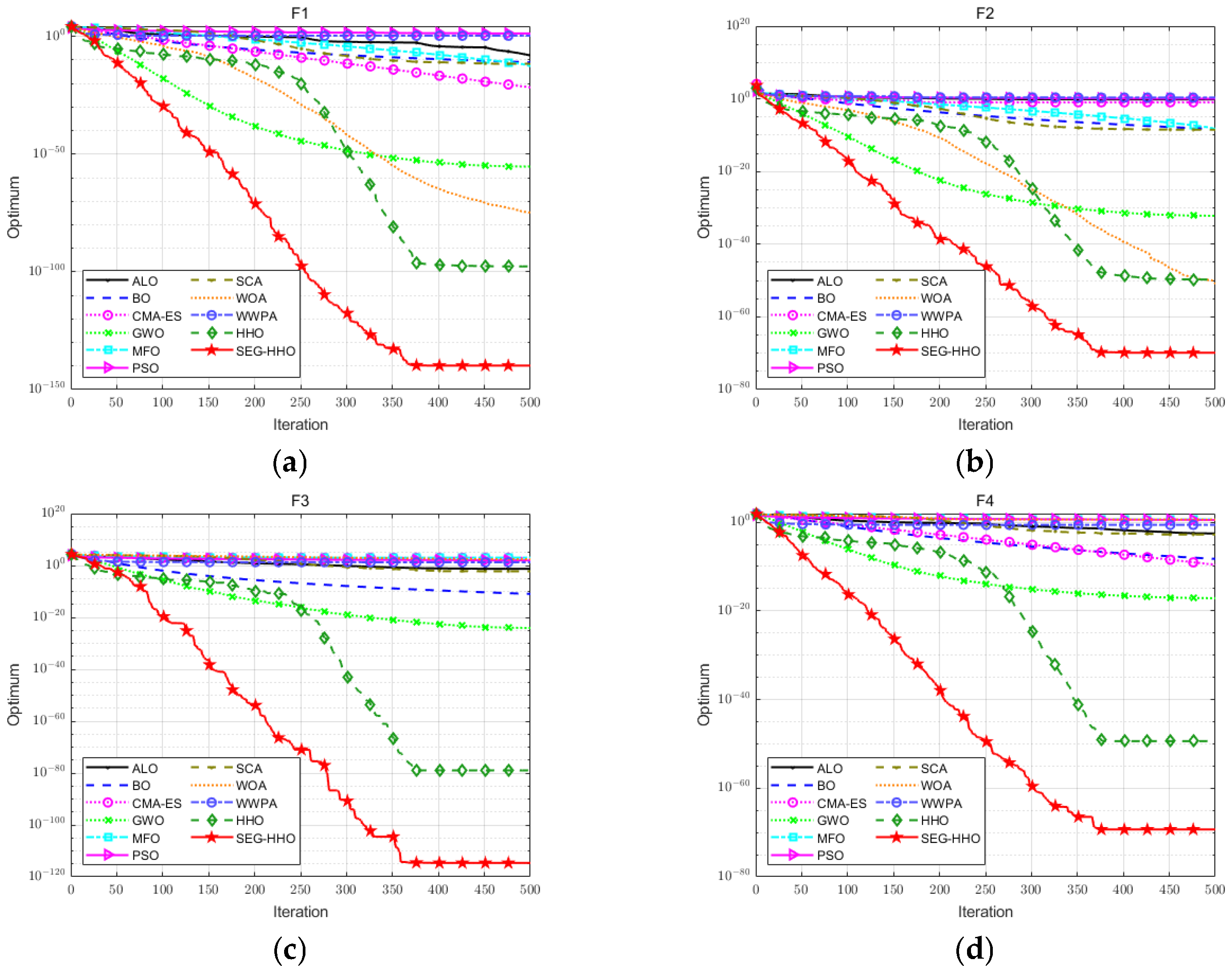
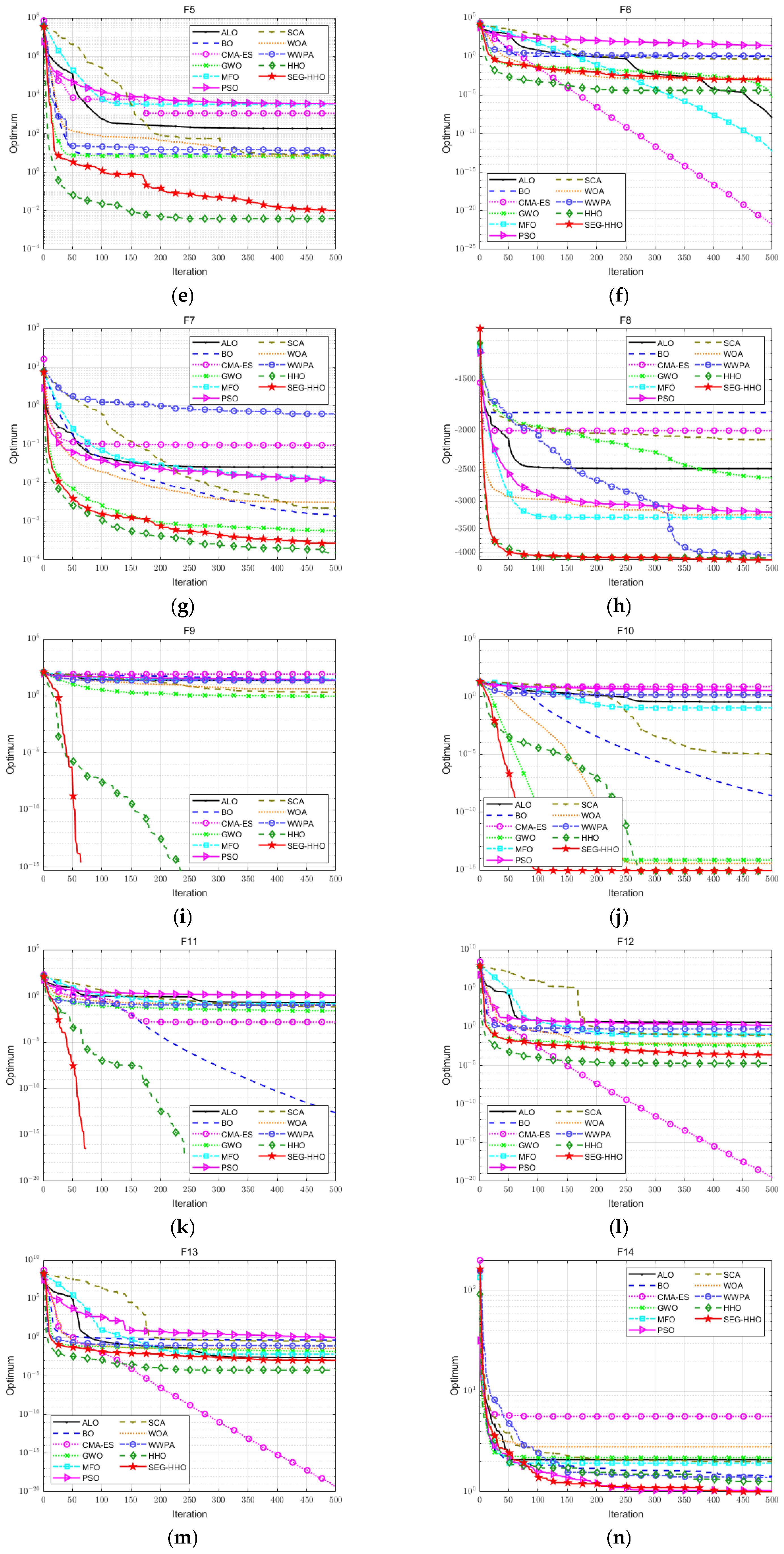
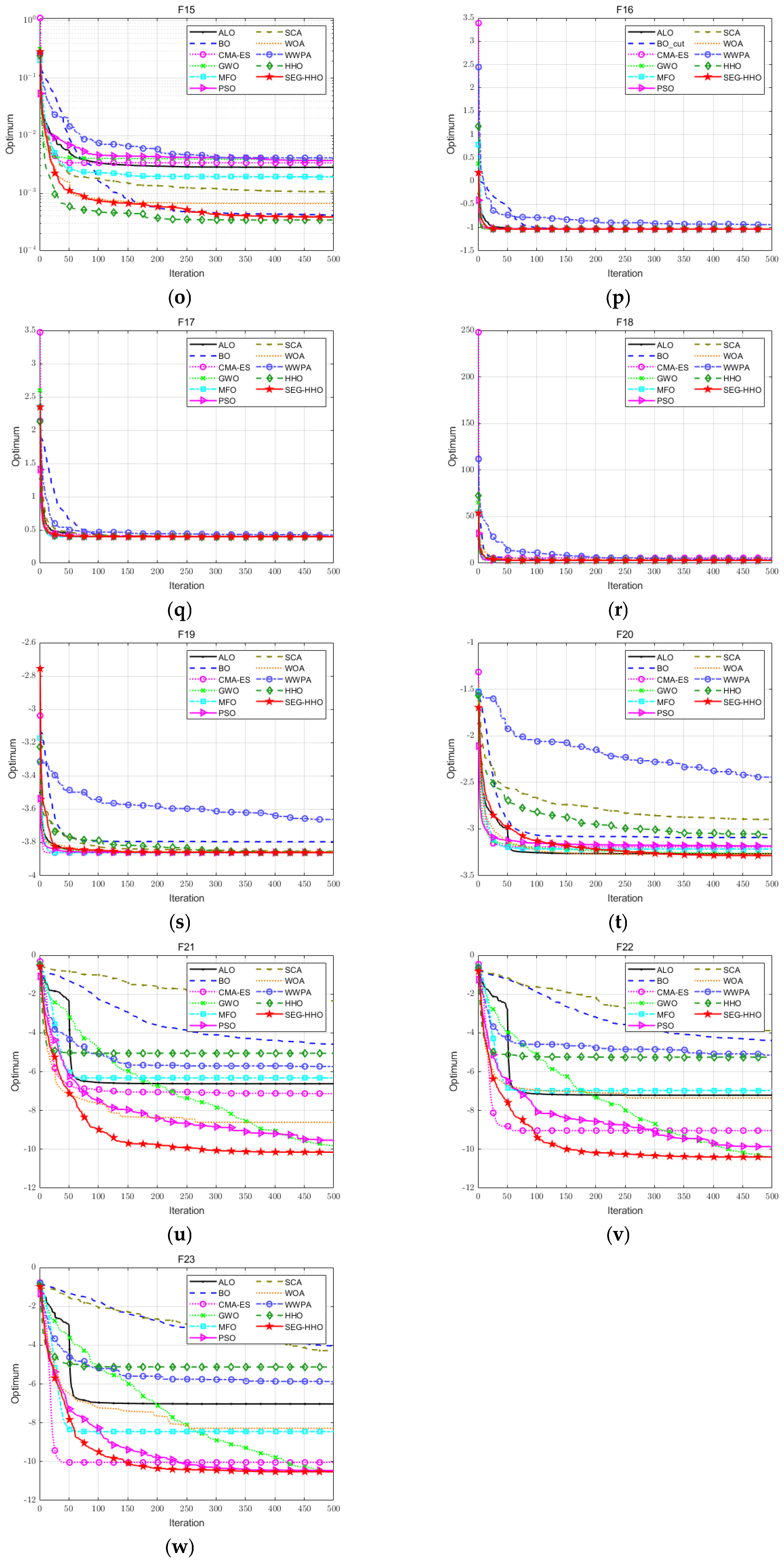
Figure 14 displays the convergence curves of all algorithms on selected functions. As can be clearly observed in this figure, the proposed SEG-HHO algorithm demonstrates superior convergence performance on the majority of the test functions.
Specifically, on unimodal functions (e.g., F1 and F2), the convergence curve of SEG-HHO descends more rapidly and converges to a lower final fitness value, indicating that its exploitation capability has been effectively enhanced. On more complex multimodal functions with numerous local optima (e.g., F9 and F11), SEG-HHO not only converges faster but is also capable of escaping local optima to find higher-quality solutions. This is attributed to its stratified evolution and hybrid search strategies, which effectively balance the algorithm’s global exploration and local exploitation capabilities. On the hybrid composite function (e.g., F21 and F23), several baseline methods, including the original HHO, suffer from early stagnation. SEG-HHO, however, sustains an active search throughout the entire iteration process and converges smoothly to a high-quality solution, demonstrating robustness in navigating complex multimodal landscapes.
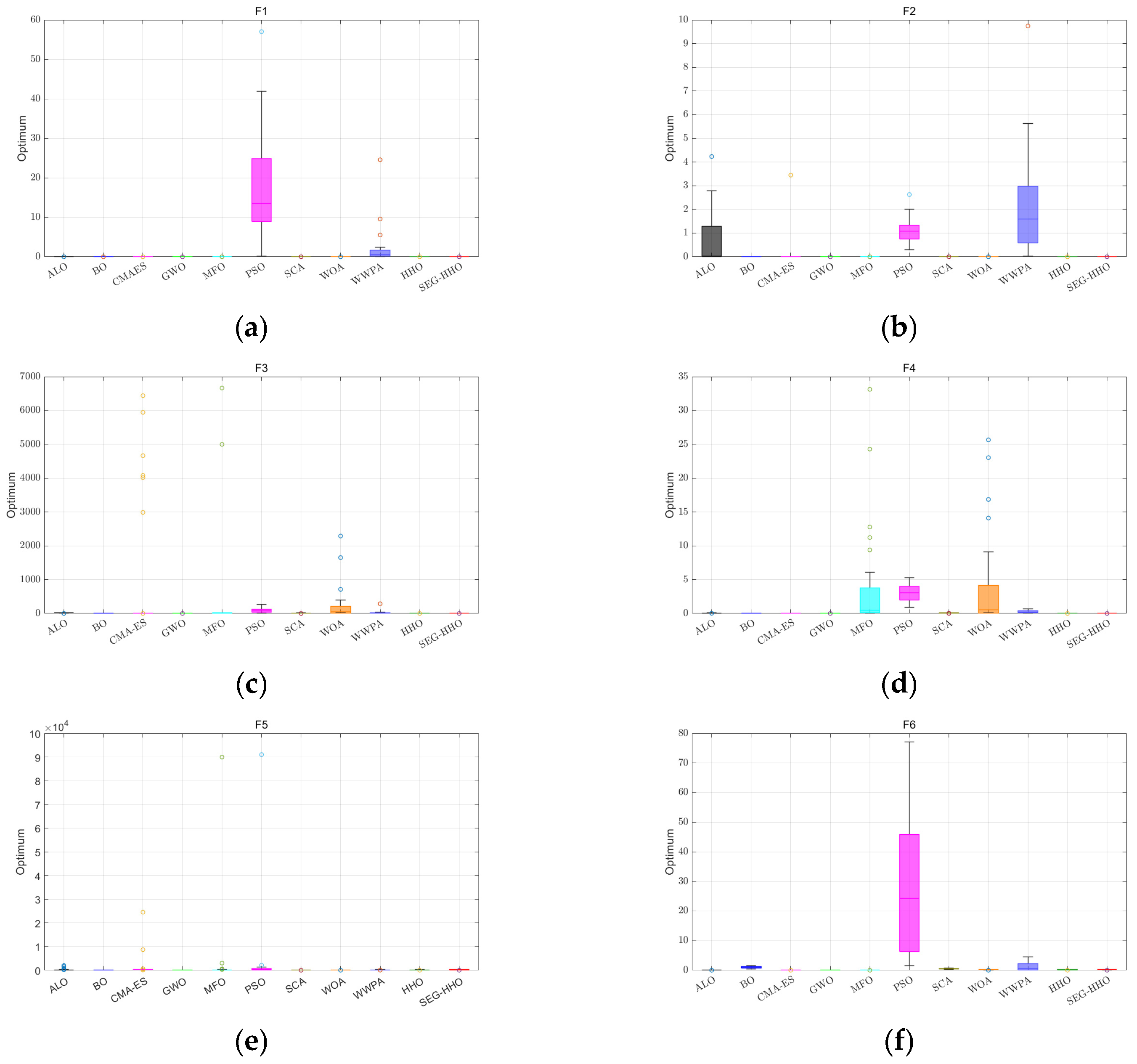
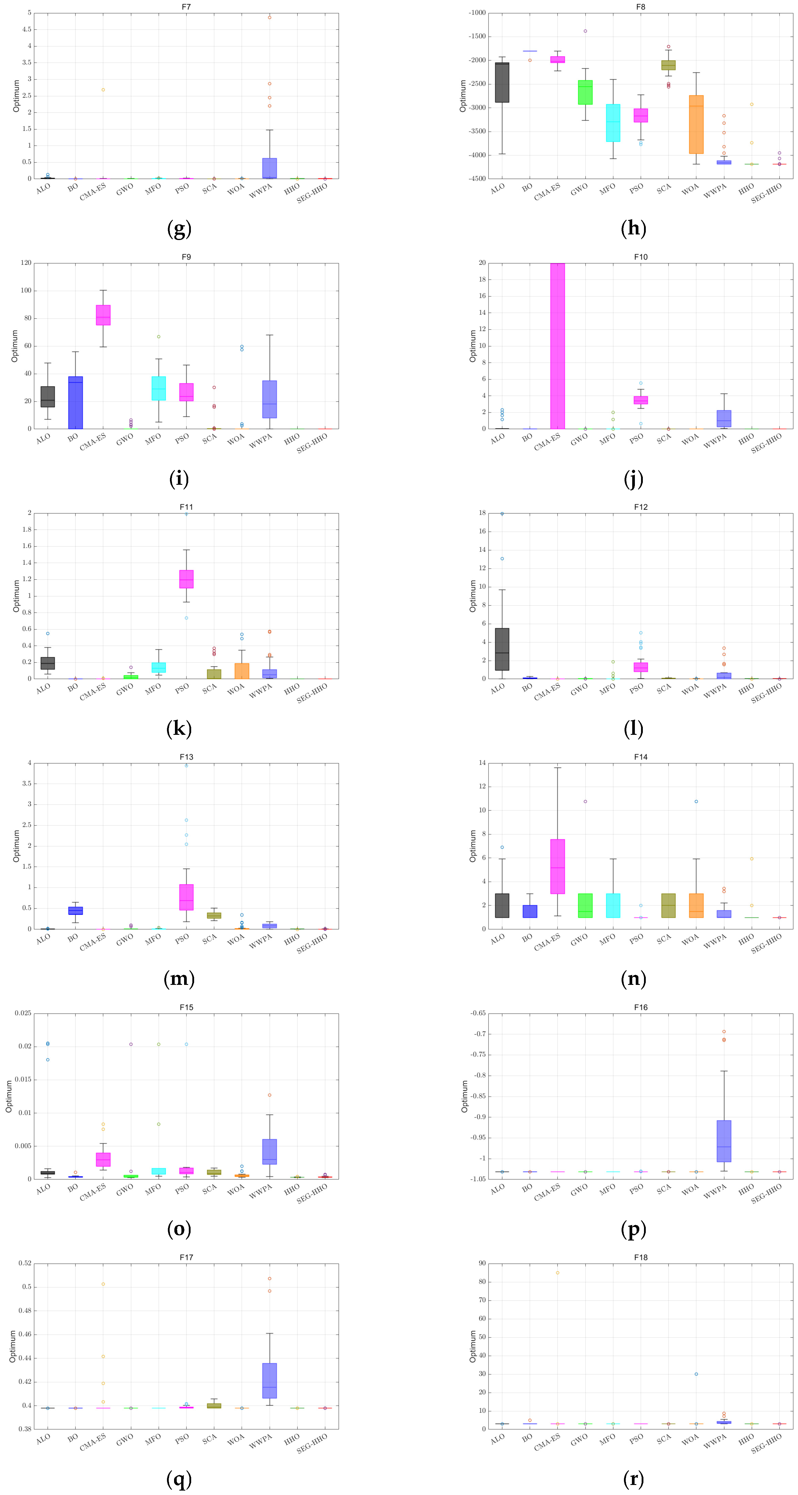
Figure 15 shows the distribution box plots of the results of each algorithm under 23 benchmark functions. It can be observed that SEG-HHO has the lowest box height among the 23 benchmark algorithms, and compared to other algorithms, SEG-HHO has fewer outliers in the result distribution, further demonstrating its advantages in convergence accuracy and stability.
In addition to optimization performance, we evaluated the computational efficiency of SEG-HHO and the baselines. Detailed runtime comparisons are provided in Appendix B (Table A1). On average, SEG-HHO requires approximately 0.15 s per run across the CEC2005 suite, which is modestly higher than simpler algorithms like SCA (0.04 s) due to its enhanced mechanisms. However, this trade-off is advantageous, as SEG-HHO delivers superior solution quality and convergence reliability, making it suitable for engineering scenarios where evaluation costs (e.g., via surrogates) are low compared to direct simulations (detailed in Section 5.4).
In summary, SEG-HHO achieves consistent and competitive convergence behavior across diverse function types, combining convergence speed, solution accuracy, and global optimization stability.

5.4. Analysis of the Optimal Assembly Scheme

To further evaluate the practical applicability of the proposed SEG-HHO algorithm in constrained engineering optimization, building on its foundational performance demonstrated in the CEC2005 benchmarks, we applied it to the gyroscope bolt assembly sequence and preload optimization problem described in prior work. This experiment highlights SEG-HHO’s capability in handling real-world constraints via our encoding–decoding mechanism, with a focus on comparing its convergence performance and final solution quality against the original HHO algorithm.
The overall optimization objective is to minimize the orthogonal axis error induced by the bolt assembly process, which is achieved by jointly optimizing the tightening sequence and the preload forces of all bolts. This contributes directly to improving the spatial attitude accuracy of the gyroscope system.
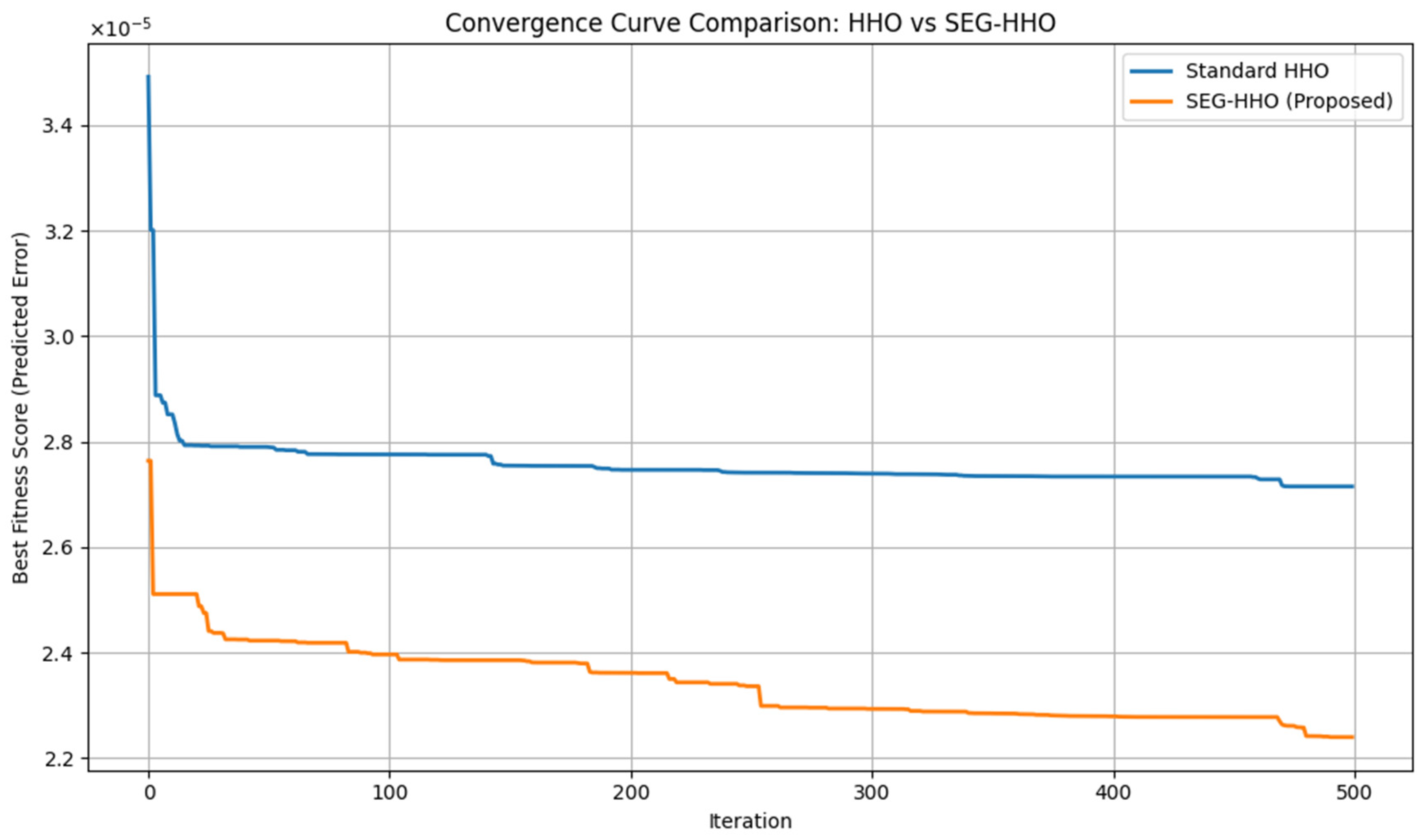
Both SEG-HHO and HHO were configured with a population size of 30 over 500 iterations. Figure 16 presents the convergence comparison. SEG-HHO not only converges faster in early stages but also continues improving during later iterations. The final fitness value reached by SEG-HHO is 2.2398 × 10⁻⁵, outperforming HHO’s result of 2.7149 × 10⁻⁵, corresponding to a relative error reduction of approximately 17.5%, computed as 2.7149 × 10 5 2.2398 × 10 5 2.7149 × 10 5 × 100 % 17.5 % .
The decoded optimal tightening plan is summarized in Table 14, detailing each tightening step, bolt ID, and assigned preload. The solution demonstrates a non-linear sequence with a balanced preload distribution ranging from 3922 N to 7500 N. Notably, the algorithm tends to assign higher preload forces in the later tightening steps while maintaining moderate loads in the initial steps. This strategy may help compensate for cumulative deviations introduced earlier, thus aiding in reducing the final orthogonal axis error.
It is worth highlighting that using high-fidelity FEM simulations as the fitness function would require approximately 15,000 evaluations (30 individuals over 500 iterations), taking over 3500 h in total and making the process computationally infeasible. In contrast, this study utilizes an AB-BiLSTM-based surrogate model to replace FEM, enabling millisecond-level evaluations and significantly reducing optimization overhead. To further quantify efficiency, runtime comparisons for SEG-HHO and HHO on this problem are detailed in Appendix B (Table A2). SEG-HHO completes in 91 s total (0.18 s per iteration), a slight increase over HHO’s 105 s due to its hybrid strategies, versus infeasible FEM-based optimization (>3500 h).
In summary, SEG-HHO, empowered by a hybrid framework that combines surrogate-based modeling with intelligent optimization, effectively solves the preload and sequencing optimization problem without relying on costly simulations, offering a practical and efficient approach for high-precision assembly systems.

6. Discussion

This study introduces and validates a data-driven optimization framework for precision bolted assembly. Our findings confirm two central hypotheses. First, by conceptualizing the bolt tightening process as a time series, our AB-BiLSTM surrogate model accurately predicted the final orthogonal axis error, significantly outperforming non-sequential models. The attention mechanism proved crucial, not as a black box, but as an interpretable tool that learned physically meaningful patterns, such as focusing on the initial and final stages of the process. Second, the proposed SEG-HHO algorithm, with its stratified population structure, demonstrated superior global search capabilities, mitigating the premature convergence often seen in standard metaheuristics when applied to complex, constrained engineering problems.
While the proposed framework shows significant promise, we acknowledge several limitations. These highlight critical gaps between simulation and real-world application, providing a clear direction for future research to address.
  • Simulation-to-Reality Gap: The current study is based entirely on high-fidelity FEM simulation data. This was a deliberate and necessary first step due to the extreme manufacturing cost and low production volume of the specialized gyroscope under study, which makes extensive physical experimentation infeasible at this early stage. This simulation-first approach allowed us to establish a robust proof-of-concept and pre-train a foundational model. The immediate and most critical next step is to bridge the simulation-to-reality gap by incorporating scarce real-world sensor data (e.g., torque readings from instrumented torque wrenches) to fine-tune and calibrate the surrogate model, enhancing its real-world applicability. Future work will also explore the impact of manufacturing tolerances (e.g., rotor coaxiality and hole clearances) and material property variations, which were simplified in the current model.
  • Generalizability and Scalability:
    (1)
    The model was validated on a specific 24-bolt gyroscope assembly. To prove broader generalizability, future work should test the framework on diverse bolt configurations and assembly structures, both in simulation and on physical systems (e.g., satellite payload assembly and semiconductor equipment). Beyond the test case, the general design of the framework enhances transferability: the AB-BiLSTM surrogate processes sequential data agnostic to specific patterns, while the SEG-HHO algorithm incorporates an encoding–decoding mechanism that decouples problem-specific constraints (e.g., symmetry and grouping) from the search procedure, enabling adaptation to new constraint types in other domains (e.g., multi-stage tightening, contact uniformity requirements, or tool accessibility constraints in aerospace assembly).
    (2)
    Regarding scalability, the inference time of the AB-BiLSTM model scales linearly with the number of bolts (O(n) complexity) [48], as RNN/LSTM architectures process sequences step-by-step. This suggests efficiency for larger systems, but current experiments are limited to 24 bolts. Scaling to more bolts (e.g., 48) or complex constraints (e.g., dynamic preload interactions) requires further validation of training time growth (potentially quadratic with dataset size expansion [48]) and overfitting risks. While the AB-BiLSTM surrogate scales efficiently, the underlying optimization problem for SEG-HHO faces exponential growth in search space with the number of bolts. To manage this complexity for larger systems, hierarchical optimization or advanced optimizers (e.g., evolutionary algorithms with adaptive operators) will be necessary.
    (3)
    Finally, cross-domain validation remains an open task. A potential roadmap includes the following: (1) within-domain tests on unseen bolt configurations (e.g., varying preload ranges or expanding to 48 bolts); (2) testing domain-specific datasets (e.g., aerospace or semiconductor assemblies); (3) recalibrating physics-based constraints to match new conditions; and (4) collaborating with industrial partners to verify transferability on real production data.
  • From Single-Objective to Multi-Objective Optimization: Our current framework minimizes orthogonal axis error as a single objective. In real-world manufacturing, engineers must balance competing objectives such as minimizing error, ensuring uniform stress distribution, reducing assembly time, and minimizing tool wear. A critical future direction is extending the framework to multi-objective optimization. This would require modifying the AB-BiLSTM surrogate to output multiple objectives (e.g., error and stress) and integrating it with optimizer algorithms like NSGA-II or an improved HHO variant. The resulting Pareto front of optimal solutions would enable engineers to make informed, context-aware decisions.
  • Path to Industrial Deployment: For practical deployment, this framework could be integrated into Computer-Aided Process Planning (CAPP) systems to generate optimal assembly plans offline. A more advanced implementation would involve creating a near real-time monitoring system on the assembly line. By integrating with IoT sensors on smart tools, the system could continuously feed live data to the AB-BiLSTM model for dynamic calibration, generating context-aware suggestions for process adjustments. This would bridge the gap between simulation predictions and physical execution, enabling iterative refinement of assembly quality.

7. Conclusions

This study successfully demonstrates that a tightly integrated framework of sequence-aware deep learning and advanced metaheuristic optimization can effectively solve complex, constrained assembly problems. We move beyond simple “compare-and-verify” approaches to offer a fully automated, data-driven optimization loop.
The key lessons learned are threefold. First, modeling the assembly process as a sequence is not just beneficial but critical for capturing the underlying physics that non-sequential models miss. Second, attention mechanisms can serve as a powerful bridge between predictive accuracy and engineering insight, revealing some certain process steps are more critical than others. Third, structured, multi-strategy optimization algorithms like SEG-HHO are essential for navigating the complex search spaces typical of real-world engineering problems, providing more robust and higher-quality solutions than their monolithic counterparts.
This work establishes a foundational component for digital twin implementation in precision manufacturing. By replacing costly physical trials or slow simulations with a fast and accurate surrogate, this approach dramatically accelerates the design-optimization cycle. The immediate path forward involves calibrating this framework with limited physical sensor data to bridge the simulation-to-reality gap. Subsequently, we aim to expand this single-objective system into a multi-objective decision-support tool. To enhance predictive power while addressing practical constraints, future work will focus on the following two key directions: developing lightweight Transformers adapted for small datasets through techniques such as transfer learning from pre-trained models and knowledge distillation and implementing model compression strategies (e.g., quantization, pruning, and parameter sharing) to enable deployment on resource-constrained systems, such as edge devices in Industrial Internet of Things (IIoT) environments.

Author Contributions

Conceptualization, D.L.; methodology, D.L. and Y.J.; validation, D.L.; formal analysis, D.L.; investigation, D.L.; resources, D.L. and H.Y.; data curation, D.L.; writing—original draft preparation, D.L.; writing—review and editing, D.L. and H.Y.; visualization, D.L.; supervision, H.Y.; project administration, D.L. and H.Y.; funding acquisition, H.Y. All authors have read and agreed to the published version of the manuscript.

Funding

This research was funded by the National Defense Basic Scientific Research Program of China, grant number JCKY2023203A004.

Data Availability Statement

The dataset used in this study was generated via high-fidelity finite element simulations. Due to confidentiality agreements with the collaborating research institute and the sensitive engineering context of the underlying CAD and simulation models, the data cannot be deposited in a public repository. However, the data are available from the corresponding author (yhg@njupt.edu.cn) upon reasonable request for academic verification purposes. The source code for the core algorithms implemented in this study is also available from the corresponding author upon reasonable request.

Conflicts of Interest

The authors declare no conflicts of interest. The funders had no role in the design of this study; in the collection, analyses, or interpretation of data; in the writing of this manuscript; or in the decision to publish the results.

Abbreviations

The following abbreviations are used in this manuscript:
FEMFinite Element Method
FEAFinite Element Analysis
LHSLatin Hypercube Sampling
SVRSupport Vector Regression
RSMResponse Surface Methodology
RNNRecurrent Neural Network
LSTMLong Short-Term Memory
GRUGated Recurrent Unit
MLPMulti-Layer Perceptron
CNNConvolutional Neural Network
AB-BiLSTMAttention-based Bidirectional Long Short-Term Memory
GAGenetic Algorithm
PSOParticle Swarm Optimization
ACOAnt Colony Optimization
ALOAnt Lion Optimizer
HHOHarris Hawks Optimization
LFLevy Flight
DEDifferential Evolution
SEG-HHOStratified Evolutionary Group-based Harris Hawks Optimization
SCASine Cosine Algorithm
BOBayesian Optimization
GWOGrey Wolf Optimizer
MFOMoth-Flame Optimization
WOAWhale Optimization Algorithm
WWPAWaterwheel Plant Algorithm
MSEMean Squared Error
MAEMean Absolute Error
RMSERoot Mean Squared Error
R2Coefficient of Determination
TPETree-structured Parzen Estimator
CAPPComputer-Aided Process Planning
IIoTIndustrial Internet of Things

Appendix A

Appendix A.1

Figure A1 visually confirms the strong linear relationship and high correlation between our model’s predictions and the ground truth, with data points clustering tightly around the y = x line.
Figure A1. Scatter plot of AB-BiLSTM.
Electronics 14 03470 g0a1

Appendix A.2

Figure A2 shows that the prediction errors are centered around zero and approximate a normal distribution, indicating that the model is well-calibrated and does not suffer from systematic bias.
Figure A2. Prediction error distribution of AB-BiLSTM.
Electronics 14 03470 g0a2

Appendix B

To provide a comprehensive view of computational efficiency, this appendix presents runtime data for the compared algorithms. All measurements are averaged over 30 independent runs in the environment described in Section 5.1.2. For brevity, CEC2005 results (Table A1) aggregate averages across all 23 functions. Standard deviations are included to reflect variability.
Table A1. Average runtime (in seconds) per run across all CEC2005 functions.
AlgorithmMean Runtime(s)Std (s)
ALO1.12730.0247
BO0.10320.0036
CMA-ES0.21000.0072
GWO0.03700.0020
MFO0.03760.0014
PSO0.05990.0024
SCA0.03600.0021
WOA0.03120.0014
WWPA0.09580.0060
HHO0.08300.0028
SEG-HHO0.15340.0060
To further quantify efficiency in the gyroscope assembly optimization problem, runtime comparisons for SEG-HHO and HHO on this problem are detailed in Table A2.
Table A2. Runtime comparison for the gyroscope assembly optimization problem (500 iterations, population size 30).
ProjectTotal Execution TimeAverage Iteration Time (s)
FEM simulationAbout 3500 hAbout 70 h
Surrogate-assisted Standard HHO104.9993 s0.2099 s
Surrogate-assisted SEG-HHO91.1565 s0.1823 s
Note: SEG-HHO’s slightly lower total time here (despite higher per-iteration complexity) results from faster convergence in practice, reducing effective iterations needed for stabilization. When paired with the AB-BiLSTM surrogate, the full framework runs in under 2 min, versus infeasible FEM-based optimization (>3500 h).

References

  1. Are Manufacturing Errors Hurting Your Business? Reliability Solutions. Available online: https://reliabilitysolutions.net/articles/the-cost-of-assembly-and-installation-errors/ (accessed on 16 August 2025).
  2. Shafi, I.; Mazhar, M.F.; Fatima, A.; Alvarez, R.M.; Miró, Y.; Espinosa, J.C.M.; Ashraf, I. Deep Learning-Based Real Time Defect Detection for Optimization of Aircraft Manufacturing and Control Performance. Drones 2023, 7, 31. [Google Scholar] [CrossRef]
  3. Li, Z.; Li, X.; Han, Y.; Zhang, P.; Zhang, Z.; Zhang, M.; Zhao, G. A Review of Aeroengines’ Bolt Preload Formation Mechanism and Control Technology. Aerospace 2023, 10, 307. [Google Scholar] [CrossRef]
  4. Zhang, J.; Wang, Y.; Wang, J.; Cao, R.; Xu, Z. Online O-Ring Stress Prediction and Bolt Tightening Sequence Optimization Method for Solid Rocket Motor Assembly. Machines 2023, 11, 387. [Google Scholar] [CrossRef]
  5. Zhang, W.; Liu, Z.; Song, Y.; Lu, Y.; Feng, Z. Prediction of Multi-Physics Field Distribution on Gas Turbine Endwall Using an Optimized Surrogate Model with Various Deep Learning Frames. Int. J. Numer. Methods Heat Fluid Flow 2023, 34, 2865–2889. [Google Scholar] [CrossRef]
  6. Kirkpatrick, S.; Gelatt, C.D.; Vecchi, M.P. Optimization by Simulated Annealing. Science 1983, 220, 671–680. [Google Scholar] [CrossRef]
  7. Marino, R. Learning from Survey Propagation: A Neural Network for MAX-E-3-SAT. Mach. Learn. Sci. Technol. 2021, 2, 035032. [Google Scholar] [CrossRef]
  8. Tatar, E.; Alper, S.E.; Akin, T. Quadrature-Error Compensation and Corresponding Effects on the Performance of Fully Decoupled MEMS Gyroscopes. J. Microelectromech. Syst. 2012, 21, 656–667. [Google Scholar] [CrossRef]
  9. Grzejda, R. Analysis of the Tightening Process of an Asymmetrical Multi-Bolted Connection. Mach. Dyn. Res. 2016, 39, 25–32. [Google Scholar]
  10. Wang, Y.; Liu, Y.; Wang, J.; Zhang, J.; Zhu, X.; Xu, Z. Research on Process Planning Method of Aerospace Engine Bolt Tightening Based on Digital Twin. Machines 2022, 10, 1048. [Google Scholar] [CrossRef]
  11. Shi, M.; Lv, L.; Sun, W.; Song, X. A Multi-Fidelity Surrogate Model Based on Support Vector Regression. Struct. Multidisc. Optim. 2020, 61, 2363–2375. [Google Scholar] [CrossRef]
  12. Gogu, C.; Passieux, J.-C. Efficient Surrogate Construction by Combining Response Surface Methodology and Reduced Order Modeling. Struct. Multidisc. Optim. 2013, 47, 821–837. [Google Scholar] [CrossRef]
  13. Zhou, Y.; Lu, Z. An Enhanced Kriging Surrogate Modeling Technique for High-Dimensional Problems. Mech. Syst. Signal Process. 2020, 140, 106687. [Google Scholar] [CrossRef]
  14. Durantin, C.; Rouxel, J.; Désidéri, J.-A.; Glière, A. Multifidelity Surrogate Modeling Based on Radial Basis Functions. Struct. Multidisc. Optim. 2017, 56, 1061–1075. [Google Scholar] [CrossRef]
  15. Li, Z.; Li, X.-C.; Wu, Z.-M.; Zhu, Y.; Mao, J.-F. Surrogate Modeling of High-Speed Links Based on GNN and RNN for Signal Integrity Applications. IEEE Trans. Microw. Theory Techn. 2023, 71, 3784–3796. [Google Scholar] [CrossRef]
  16. Xu, L.; Xu, Y.; Wang, K.; Ye, L.; Zhang, W. Two-Stream Bolt Preload Prediction Network Using Hydraulic Pressure and Nut Angle Signals. Eng. Appl. Artif. Intell. 2024, 136, 109029. [Google Scholar] [CrossRef]
  17. Li, X.; Peng, C.; Zhao, Y.; Xia, X. A Hybrid DSCNN-GRU Based Surrogate Model for Transient Groundwater Flow Prediction. Appl. Sci. 2025, 15, 4576. [Google Scholar] [CrossRef]
  18. Song, B.; Liu, Y.; Fang, J.; Liu, W.; Zhong, M.; Liu, X. An Optimized CNN-BiLSTM Network for Bearing Fault Diagnosis under Multiple Working Conditions with Limited Training Samples. Neurocomputing 2024, 574, 127284. [Google Scholar] [CrossRef]
  19. Xie, Y.; Wu, D.; Qiang, Z. A Unifying View for the Mixture Model of Sparse Gaussian Processes. Inf. Sci. 2024, 660, 120124. [Google Scholar] [CrossRef]
  20. Schweidtmann, A.M.; Bongartz, D.; Grothe, D.; Kerkenhoff, T.; Lin, X.; Najman, J.; Mitsos, A. Deterministic Global Optimization with Gaussian Processes Embedded. Math. Prog. Comp. 2021, 13, 553–581. [Google Scholar] [CrossRef]
  21. Zhongbo, Y.; Hien, P.L. Pre-Trained Transformer Model as a Surrogate in Multiscale Computational Homogenization Framework for Elastoplastic Composite Materials Subjected to Generic Loading Paths. Comput. Methods Appl. Mech. Eng. 2024, 421, 116745. [Google Scholar] [CrossRef]
  22. Wan, X.; Liu, K.; Qiu, W.; Kang, Z. An Assembly Sequence Planning Method Based on Multiple Optimal Solutions Genetic Algorithm. Mathematics 2024, 12, 574. [Google Scholar] [CrossRef]
  23. Zheng, Y.; Chen, L.; Wu, D.; Jiang, P.; Bao, J. Assembly Sequence Planning Method for Optimum Assembly Accuracy of Complex Products Based on Modified Teaching–Learning Based Optimization Algorithm. Int. J. Adv. Manuf. Technol. 2023, 126, 1681–1699. [Google Scholar] [CrossRef]
  24. Malek, N.G.; Eslamlou, A.D.; Peng, Q.; Huang, S. Effective GA Operator for Product Assembly Sequence Planning. Comput.-Aided Des. Appl. 2024, 21, 713–728. [Google Scholar] [CrossRef]
  25. Zhang, W. Assembly Sequence Intelligent Planning Based on Improved Particle Swarm Optimization Algorithm. Manuf. Technol. 2023, 23, 557–563. [Google Scholar] [CrossRef]
  26. Ab Rashid, M.F.F.; Tiwari, A.; Hutabarat, W. Integrated Optimization of Mixed-Model Assembly Sequence Planning and Line Balancing Using Multi-Objective Discrete Particle Swarm Optimization. Artif. Intell. Eng. Des. Anal. Manuf. 2019, 33, 332–345. [Google Scholar] [CrossRef]
  27. Yang, J.; Liu, F.; Dong, Y.; Cao, Y.; Cao, Y. Multiple-Objective Optimization of a Reconfigurable Assembly System via Equipment Selection and Sequence Planning. Comput. Ind. Eng. 2022, 172, 108519. [Google Scholar] [CrossRef]
  28. Han, Z.; Wang, Y.; Tian, D. Ant Colony Optimization for Assembly Sequence Planning Based on Parameters Optimization. Front. Mech. Eng. 2021, 16, 393–409. [Google Scholar] [CrossRef]
  29. Tseng, H.-E.; Chang, C.-C.; Lee, S.-C.; Huang, Y.-M. Hybrid Bidirectional Ant Colony Optimization (Hybrid BACO): An Algorithm for Disassembly Sequence Planning. Eng. Appl. Artif. Intell. 2019, 83, 45–56. [Google Scholar] [CrossRef]
  30. Xing, Y.; Wu, D.; Qu, L. Parallel Disassembly Sequence Planning Using Improved Ant Colony Algorithm. Int. J. Adv. Manuf. Technol. 2021, 113, 2327–2342. [Google Scholar] [CrossRef]
  31. Heidari, A.A.; Mirjalili, S.; Faris, H.; Aljarah, I.; Mafarja, M.; Chen, H. Harris Hawks Optimization: Algorithm and Applications. Future Gener. Comput. Syst. 2019, 97, 849–872. [Google Scholar] [CrossRef]
  32. Devan, P.A.M.; Ibrahim, R.; Omar, M.; Bingi, K.; Abdulrab, H. A Novel Hybrid Harris Hawk-Arithmetic Optimization Algorithm for Industrial Wireless Mesh Networks. Sensors 2023, 23, 6224. [Google Scholar] [CrossRef]
  33. Yagmur, N.; Dag, İ.; Temurtas, H. Classification of Anemia Using Harris Hawks Optimization Method and Multivariate Adaptive Regression Spline. Neural Comput. Appl. 2024, 36, 5653–5672. [Google Scholar] [CrossRef]
  34. Pavan, G.; Ramesh Babu, A. Enhanced Randomized Harris Hawk Optimization of PI Controller for Power Flow Control in the Microgrid with the PV-Wind-Battery System. Sci. Technol. Energy Transit. 2024, 79, 45. [Google Scholar] [CrossRef]
  35. Ryalat, M.H.; Dorgham, O.; Tedmori, S.; Al-Rahamneh, Z.; Al-Najdawi, N.; Mirjalili, S. Harris Hawks Optimization for COVID-19 Diagnosis Based on Multi-Threshold Image Segmentation. Neural Comput. Appl. 2023, 35, 6855–6873. [Google Scholar] [CrossRef] [PubMed]
  36. Akl, D.T.; Saafan, M.M.; Haikal, A.Y.; El-Gendy, E.M. IHHO: An Improved Harris Hawks Optimization Algorithm for Solving Engineering Problems. Neural Comput. Appl. 2024, 36, 12185–12298. [Google Scholar] [CrossRef]
  37. Ni, J.; Tang, W.C.; Pan, M.; Qiu, X.; Xing, Y. Assembly Sequence Optimization for Minimizing the Riveting Path and Overall Dimensional Error. Proc. Inst. Mech. Eng. Part B J. Eng. Manuf. 2017, 232, 2605–2615. [Google Scholar] [CrossRef]
  38. Xu, X.; Li, J.; Yang, Y.; Shen, F. Toward Effective Intrusion Detection Using Log-Cosh Conditional Variational Autoencoder. IEEE Internet Things J. 2021, 8, 6187–6196. [Google Scholar] [CrossRef]
  39. Mirjalili, S. The Ant Lion Optimizer. Adv. Eng. Softw. 2015, 83, 80–98. [Google Scholar] [CrossRef]
  40. Frazier, P.I. A Tutorial on Bayesian Optimization. arXiv 2018, arXiv:1807.02811. [Google Scholar] [CrossRef]
  41. Hansen, N. The CMA Evolution Strategy: A Tutorial. arXiv 2016, arXiv:1604.00772. [Google Scholar] [CrossRef]
  42. Mirjalili, S.; Mirjalili, S.M.; Lewis, A. Grey Wolf Optimizer. Adv. Eng. Softw. 2014, 69, 46–61. [Google Scholar] [CrossRef]
  43. Mirjalili, S. Moth-Flame Optimization Algorithm: A Novel Nature-Inspired Heuristic Paradigm. Knowl.-Based Syst. 2015, 89, 228–249. [Google Scholar] [CrossRef]
  44. Wang, D.; Tan, D.; Liu, L. Particle Swarm Optimization Algorithm: An Overview. Soft Comput. 2018, 22, 387–408. [Google Scholar] [CrossRef]
  45. Mirjalili, S. SCA: A Sine Cosine Algorithm for Solving Optimization Problems. Knowl.-Based Syst. 2016, 96, 120–133. [Google Scholar] [CrossRef]
  46. Mirjalili, S.; Lewis, A. The Whale Optimization Algorithm. Adv. Eng. Softw. 2016, 95, 51–67. [Google Scholar] [CrossRef]
  47. Abdelhamid, A.A.; Towfek, S.K.; Khodadadi, N.; Alhussan, A.A.; Khafaga, D.S.; Eid, M.M.; Ibrahim, A. Waterwheel Plant Algorithm: A Novel Metaheuristic Optimization Method. Processes 2023, 11, 1502. [Google Scholar] [CrossRef]
  48. Kratzert, F.; Klotz, D.; Shalev, G.; Klambauer, G.; Hochreiter, S.; Nearing, G. Benchmarking a Catchment-Aware Long Short-Term MemoryNetwork (LSTM) for Large-Scale Hydrological Modeling. Hydrol. Earth Syst. Sci. Discuss. 2019, 2019, 1–32. [Google Scholar]
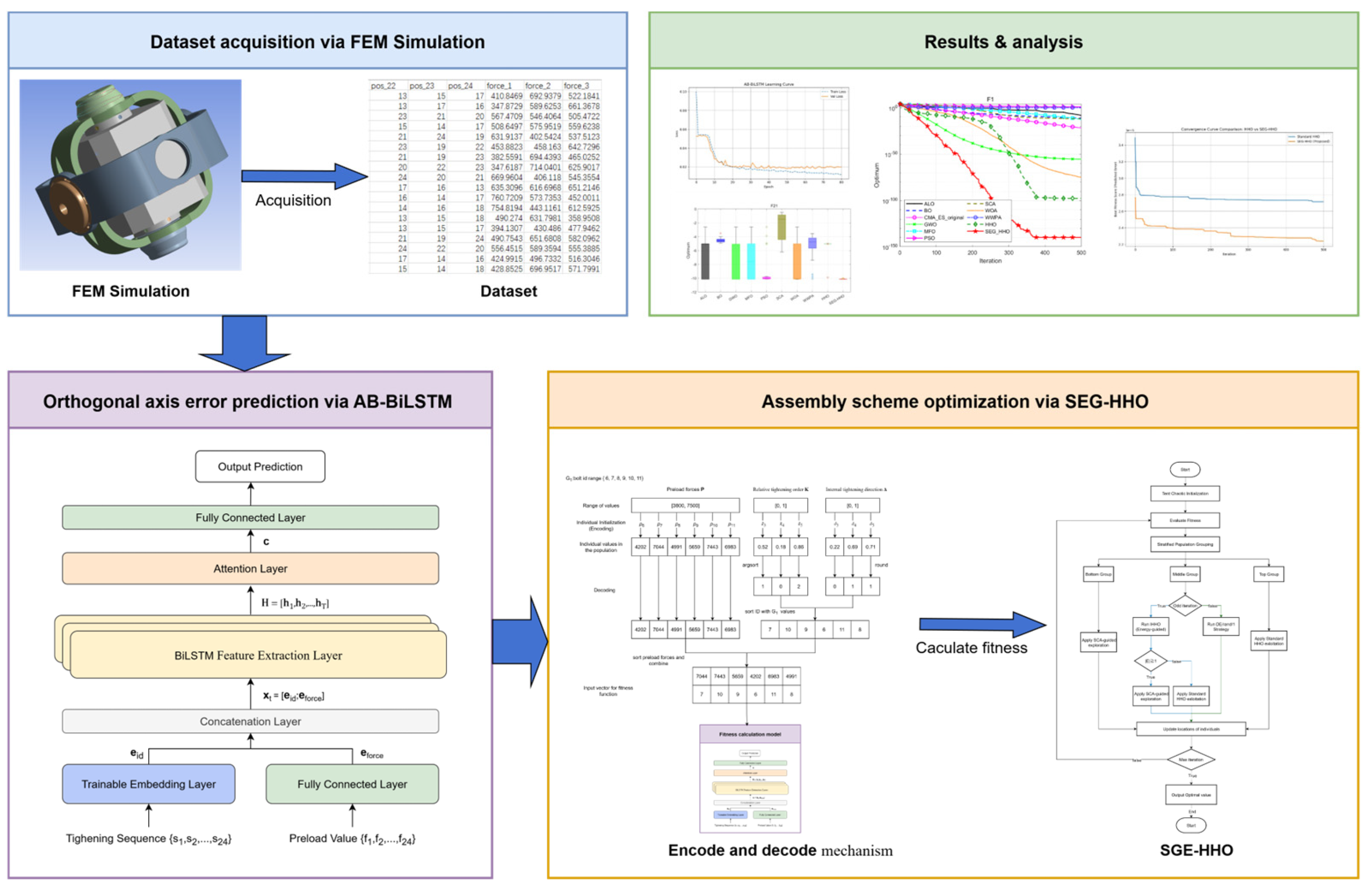
Figure 1. Framework overview.
Electronics 14 03470 g001
Figure 2. Gyroscope model in ANSYS: (a) different components of the inertial gyroscope; (b) 24 key bolts are displayed in green (highlighted by ANSYS to indicate the bolt models).
Electronics 14 03470 g002
Figure 3. The total architecture of AB-BiLSTM.
Electronics 14 03470 g003
Figure 4. Flowchart of SEG-HHO. The blue line represents odd iterations, and the green line represents even iterations.
Electronics 14 03470 g004
Figure 5. Conceptual diagram of the encoding–decoding mechanism.
Electronics 14 03470 g005
Figure 6. Encoding and decoding mechanisms with a concrete numerical example.
Electronics 14 03470 g006
Figure 7. The loss curve of the proposed AB-BiLSTM.
Electronics 14 03470 g007
Figure 8. Non-linear drop of R2.
Electronics 14 03470 g008
Figure 9. Attention visualization heatmap.
Electronics 14 03470 g009
Figure 10. Preload curve with attention weights for sample 15.
Electronics 14 03470 g010
Figure 11. Correlation between ΔPreload and ΔAttention.
Electronics 14 03470 g011
Figure 12. Boxplot of the variance of attention changes.
Electronics 14 03470 g012
Figure 13. MAE comparison across models under different noise levels.
Electronics 14 03470 g013
Figure 14. Convergence curves of SEG-HHO and comparative algorithms on representative functions from CEC2005. (a): F1; (b): F2; (c): F3; (d): F4; (e): F5; (f): F6; (g): F7; (h): F8; (i): F9; (j): F10; (k): F11; (l): F12; (m): F13; (n): F14; (o): F15; (p): F16; (q): F17; (r): F18; (s): F19; (t): F20 (u): F21; (v): F22; (w): F23.
Electronics 14 03470 g014aElectronics 14 03470 g014bElectronics 14 03470 g014c
Figure 15. Boxplot of solution distributions for all algorithms on 23 CEC2005 benchmark functions. Colors are used only for visual distinction among the algorithms. (a): F1; (b): F2; (c): F3; (d): F4; (e): F5; (f): F6; (g): F7; (h): F8; (i): F9; (j): F10; (k): F11; (l): F12; (m): F13; (n): F14; (o): F15; (p): F16; (q): F17; (r): F18; (s): F19; (t): F20 (u): F21; (v): F22; (w): F23.
Electronics 14 03470 g015aElectronics 14 03470 g015bElectronics 14 03470 g015c
Figure 16. Convergence curve of SEGHHO and standard HHO.
Electronics 14 03470 g016
Table 1. R2 scores of models with/without initial preload.
ModelsWithout Initial PreloadWith Initial Preload
RNN0.29250.1693
LSTM0.5651−0.0165
BiLSTM0.5353−0.0311
Table 2. Input–output format of the AB-BiLSTM model.
ComponentDescriptionData Type/DimensionNormalization/Encoding
Bolt ID SequenceOrder of bolts tightened in processInteger, length 24Trainable embedding (dim = 32)
Preload SequenceFinal preload value for each boltFloat, length 24Z-score normalization
OutputPredicted orthogonal axis errorFloat, scalarlog(1 + p) + Min–Max normalization
Table 3. Summary of SEG-HHO evolutionary phases.
Group (Fitness-Based)Primary Goal (Intuitive Explanation)Core Mechanism
Top GroupDeep Exploitation: Quickly refine the best-known solutions.Standard HHO’s highly efficient “Besiege” strategies.
Middle GroupBalanced Search: Adaptively explore new regions while also exploiting promising ones.Alternating Hybrid Strategy: HHO for exploitation and Differential Evolution (DE) for injecting diversity.
Bottom GroupBroad Exploration: Search widely to escape local optima and discover entirely new promising areas.Sine Cosine Algorithm (SCA) guided the search for structured, wave-like exploration.
Table 4. Comparison of SEG-HHO with HHO, DE, and SCA.
AlgorithmCore IdeaExploration StrategyExploitation StrategyKey Contribution in SEG-HHO
HHOMimics cooperative hunting of hawks.Hawks track prey based on random perches or average location.Four “besiege” strategies based on prey energy.Provides the foundational framework and powerful exploitation operators (used by Top and Middle Groups).
DEUses vector differences between individuals to create new candidates.“DE/rand/1” mutation creates diverse trial vectors.Crossover and selection retain better solutions.Injects significant population diversity to prevent stagnation (used by Middle Group).
SCAUses sine/cosine functions to explore/exploit space around the best solution.Large-amplitude oscillations for global search.Small-amplitude oscillations for local search.Provides a structured, directional exploration mechanism, superior to random walks (used by Bottom Group).
SEG-HHOStratified, multi-strategy co-evolution.Systematic and layered: SCA for broad search (Bottom); DE for diversity (Middle).Focused and intensified: Standard HHO for deep exploitation (Top); HHO for refinement (Middle).Synthesizes the strengths of HHO, DE, and SCA into a cohesive, role-based framework that dynamically balances the search.
Table 5. Hyperparameter search space for Optuna.
HyperparameterSearch Range/Type
Batch SizeCategorical [16, 32, 64, 128]
Learning RateLog-uniform [1e−5, 1e−3]
OptimizerCategorical [Adam, AdamW]
Number of LayersInteger [1, 5]
Embedding DimensionCategorical [16, 32, 64, 128]
Hidden DimensionCategorical [32, 64, 128, 256]
Dropout RateCategorical [0.0, 0.1, 0.2, 0.3]
Table 6. Optimal hyperparameter configuration for the AB-BiLSTM model.
Value
Batch Size16
Learning Rate8.8051E−5
OptimizerAdamW (weight_decay = 1e−4)
Num of Layers5
Embed Dimension32
Hidden Dimension256
Dropout Rate0.1
Table 7. Architectural parameter configurations for all comparative models.
ModelArchitecture ConfigurationKey Hyperparameters
MLPFlatten () → Dense (256, ReLU) → Dropout (0.1) → Dense (128, ReLU) → Dropout (0.1) → Dense (1, Softplus)Neurons: 256 (L1), 128 (L2)
Dropout: 0.1
1D-CNNConv1D (256, kernel = 3, ReLU) → Dropout (0.1) →
Conv1D (256, kernel = 3, ReLU) → AdaptiveAvgPool1D (1) → Flatten () → Dense (1, Softplus)
Filters: 256
Kernel: 3
Dropout: 0.1
RNNEmbedding (32) → RNN (256, dropout = 0.1) × 5 → Dense (1, Softplus)Embed Dim: 32
Hidden Dim: 256
Layers: 5
Dropout: 0.1
LSTMEmbedding (32) → LSTM (256, dropout = 0.1) × 5 → Dense (1, Softplus)Embed Dim: 32
Hidden Dim: 256
Layers: 5
Dropout: 0.1
BiLSTMEmbedding (32) → BiLSTM (256, dropout = 0.1) × 5 → Dense (1, Softplus)Embed Dim: 32
Hidden Dim: 256
Layers: 5
Dropout: 0.1
Table 8. Test performance of the models.
ModelMSERMSEMAER2Latency (ms)Train Time (s)
AB-BiLSTM2.8444E−095.3333E−053.5949E−050.81731.175323189.8061
BiLSTM3.0872E−095.5562E−053.7415E−050.80171.256722224.274
MLP1.5446E−081.2428E−049.8472E−050.00791.13091455.7333
1D-CNN1.5641E−081.2506E−049.8688E−05−0.00451.02167768.3319
RNN1.4731E−081.2137E−049.5717E−050.05381.00786560.1832
LSTM2.9932E−095.4710E−053.6671E−050.80771.357545175.3624
GRU2.9833E−095.4619E−053.6816E−050.80831.362813155.0558
Note: The values in bold highlight the optimal performance achieved for each respective metric.
Table 9. Comparison results of FEM vs. AB-BiLSTM.
ProjectValue
ANSYS Average Simulation Time14 min/Sample
AB-BiLSTM Single Sample Prediction Time1.3413 (ms)
Total Training Time 189.8061 (s)
Model Accuracy (MAE)3.5949E−05
Speedup Ratio714,711
Table 10. Result of ablation study.
AB-BiLSTMBiLSTMImprovement
MSE2.8444E−093.0872E−098.54%
RMSE5.3333E−055.5562E−054.18%
MAE3.5949E−053.7415E−053.92%
R20.81730.80171.95%
Note: The values in bold highlight the optimal performance achieved for each respective metric.
Table 11. Detailed performance metrics of models under varying noise levels.
Noise LevelModelRMSEMAER2
1%AB-BiLSTM6.3361E−053.9414E−050.7282
BiLSTM6.5385E−054.0155E−050.7165
MLP1.2535E−049.8554E−05−0.0053
1D-CNN1.2792E−041.0122E−04−0.0469
RNN1.2701E−049.7619E−05−0.0321
LSTM6.6070E−054.1412E−050.7107
GRU6.5368E−054.1342E−050.7166
5%AB-BiLSTM6.3589E−053.9748E−050.7263
BiLSTM6.5466E−054.1059E−050.7258
MLP1.2779E−041.0108E−04−0.0448
1D-CNN1.2535E−049.8513E−05−0.0052
RNN1.2699E−049.7622E−05−0.0317
LSTM6.7211E−054.2610E−050.7110
GRU6.5344E−054.1658E−050.7168
10%AB-BiLSTM6.7938E−054.1324E−050.7047
BiLSTM6.7908E−054.3254E−050.7150
MLP1.2775E−041.0095E−04−0.0441
1D-CNN1.2536E−049.8523E−05−0.0054
RNN1.2699E−049.7630E−05−0.0317
LSTM6.8729E−054.3845E−050.6978
GRU6.6685E−054.3753E−050.7050
15%AB-BiLSTM6.9643E−054.4518E−050.6897
BiLSTM6.9893E−054.6727E−050.6875
MLP1.2816E−041.0136E−04−0.0508
1D-CNN1.2537E−049.8543E−05−0.0056
RNN1.2737E−049.8130E−05−0.0379
LSTM6.8646E−054.5889E−050.6885
GRU6.9545E−054.5893E−050.6806
Note: The values in bold highlight the optimal performance achieved for each respective metric.
Table 12. Test functions.
FunctionDimensionDomainTheoretical Optimum
F 1 x = i = 1 n   x i 2 30 [ 100,100 ] 0
F 2 x = i = 1 n   x i + i = 1 n   x i 30 [ 10,10 ] 0
F 3 x = i = 1 n   j = 1 i   x j 2 30 [ 100,100 ] 0
F 4 x = m a x i   x i , 1 i n 30 [ 100,100 ] 0
F 5 x = i = 1 n 1   100 x i + 1 x i 2 2 + x i 1 2 30 [ 30,30 ] 0
F 6 x = i = 1 n   x i + 0.5 2 30 [ 100,100 ] 0
F 7 x = i = 1 n   i x i 4 + r a n d o m [ 0,1 ) 30 [ 1.28,1.28 ] 0
F 8 x = i = 1 n   x i s i n | x i | 30 [ 500,500 ] −12,569.4
F 9 x = i = 1 n   x i 2 10 c o s 2 π x i + 10 30 [ 5.12,5.12 ] 0
F 10 x = 20 e x p 0.2 1 n i = 1 n   x i 2 e x p 1 n i = 1 n   c o s 2 π x i + 20 + e 30 [ 32,32 ] 0
F 11 x = 1 4000 i = 1 n   x i 2 i = 1 n   c o s x i i + 1 30 [ 600,600 ] 0
F 12 x = π n 10 s i n ( π y 1 ) + i = 1 n 1   ( y i 1 ) 2 1 + 10 s i n 2 ( π y i + 1 ) + y n 1 2 + i = 1 n   u ( x i , 10,100 , 4 ) 30 [ 50,50 ] 0
F 13 x = 0.1 s i n 2 3 π x i + i = 1 n   x i 1 2 1 + s i n 2 3 π x i + 1 30 [ 50,50 ] 0
F 14 x = 1 500 + j = 1 25   1 j + i = 1 2   x i a i j 6 1 2 [ 65,65 ] 1
F 15 x = i = 1 11   a i x i b i 2 + b 1 x 2 b i 2 + b 1 x 3 + x 4 2 4 [ 5,5 ] 0.00003075
F 16 x = 4 x 1 2 2.1 x 1 4 + 1 3 x 1 6 + x 1 x 2 4 x 2 2 + 4 x 2 4 2 [ 5,5 ] −1.0316285
F 17 x = x 2 5.1 4 π 2 x 1 2 + 5 π x 1 6 2 + 10 1 1 8 π c o s x 1 + 10 2 [ 5,5 ] 0.398
F 18 x = 1 + x 1 + x 2 + 1 2 19 14 x 1 + 3 x 1 2 14 x 2 + 6 x 1 x 2 + 3 x 2 2 × 30 + 2 x 1 3 x 2 2 × 18 32 x 1 + 12 x 1 2 + 48 x 2 36 x 1 x 2 + 27 x 2 2 2 [ 2,2 ] 3
F 19 x = i = 1 4   c i e x p j = 1 3   a i j x j p i j 2 3 [ 0,1 ] −3.86
F 20 x = i = 1 4   c i e x p j = 1 6   a i j x j p i j 2 6 [ 0,1 ] −3.32
F 21 x = i = 1 5   X a i X a i T + c i 1 4 [ 0,10 ] −10
F 22 x = i = 1 7   X a i X a i T + c i 1 4 [ 0,10 ] −10
F 23 x = i = 1 10   X a i X a i T + c i 1 4 [ 0,10 ] −10
Table 13. Performance comparison of SEG-HHO and nine metaheuristic algorithms on the CEC2005 test suite (30 independent runs).
Function SEG-HHOHHOALOBOCMA-ESGWOMFOPSOSCAWOAWWPA
F1Mean4.0221E−1394.3237E−971.2531E−081.0253E−112.1337E−223.3835E−574.5905E−131.7904E+011.0187E−115.0654E−759.6433E−01
Std2.1893E−1382.2390E−961.2114E−081.3546E−121.8426E−229.5492E−571.2655E−121.6916E+014.2301E−112.7739E−741.9933
Min1.6133E−1719.5971E−1154.3733E−097.3048E−121.3552E−231.8406E−603.4952E−152.54177.2846E−199.8147E−921.4099E−05
Max1.1994E−1371.2279E−954.9236E−081.1980E−117.7019E−224.9406E−566.1571E−127.6199E+012.2515E−101.5193E−739.7573E+00
Rank1298546117310
F2Mean1.3457E−731.8175E−504.3569E−014.4464E−091.1494E−017.4493E−336.7998E−091.85761.7365E−091.1527E−502.1362
Std4.4841E−739.4932E−508.8104E−014.1546E−106.2953E−011.5590E−329.5554E−092.54863.8080E−096.2569E−501.7541
Min8.8058E−887.5733E−622.1778E−053.2226E−093.6201E−123.5334E−354.3657E−103.6887E−011.1886E−125.1848E−597.0394E−02
Max1.9042E−725.2069E−493.2766E+005.0923E−093.44817.9383E−323.9520E−081.1626E+012.0214E−083.4280E−495.6360
Rank1396847105211
F3Mean2.2224E−1138.3627E−877.5129E−021.0715E−118.5932E+021.5744E−247.5142E−027.3812E+015.2861E−032.5802E+021.8125E+01
Std1.2173E−1123.3771E−862.8736E−011.4833E−122.4910E+034.1683E−241.1806E−017.5241E+012.5573E−026.0142E+023.5604E+01
Min3.0890E−1631.5349E−1031.1691E−056.6643E−123.3521E−162.4941E−303.0860E−043.40351.9934E−072.7756E−011.9237E−02
Max6.6672E−1121.7628E−851.55591.3073E−111.1638E+041.9458E−234.9815E−013.8305E+021.4050E−013.0595E+031.8765E+02
Rank1264113795108
F4Mean1.2864E−702.5824E−507.5664E−035.1141E−092.4604E−102.3031E−182.36343.13494.8785E−045.31392.8517E−01
Std4.1288E−706.2700E−502.6260E−025.6416E−101.3137E−104.7874E−184.72091.38797.8757E−049.85752.4805E−01
Min2.4386E−884.7659E−591.2017E−043.6044E−097.4107E−118.6002E−212.5910E−037.9789E−011.9837E−064.4480E−031.5187E−02
Max1.7298E−693.0726E−491.4461E−016.2106E−095.4165E−102.4514E−172.0960E+016.16953.5907E−034.1523E+019.2019E−01
Rank1275439106118
F5Mean1.3699E−023.6246E−031.4427E+028.93751.1373E+036.88062.9057E+028.7679E+027.39771.4575E+013.4891E+01
Std2.0436E−026.5977E−033.0888E+022.2660E−024.6894E+036.1221E−017.5627E+029.4807E+023.9958E−014.2675E+019.8493E+01
Min1.1309E−047.3646E−083.3591E−048.88102.8821E−025.59975.3872E−016.5256E+016.72256.06506.3616E−02
Max8.1651E−022.6413E−021.4097E+038.98302.4505E+048.06883.0219E+033.5664E+038.71272.4052E+025.4888E+02
Rank2185113910467
F6Mean7.1125E−043.9286E−059.5960E−091.16601.8457E−228.3539E−032.1482E−131.9341E+014.4334E−011.1771E−031.5115
Std1.0798E−034.8862E−057.3957E−093.6229E−011.8178E−224.5738E−023.4699E−132.0632E+011.2892E−011.8088E−032.7255
Min2.7693E−062.1451E−081.4970E−096.0281E−012.2973E−231.3786E−061.6529E−166.5394E−011.3759E−011.6681E−046.4583E−04
Max4.8326E−031.8459E−043.2171E−081.91527.1981E−222.5052E−011.3355E−129.3079E+017.9438E−019.3304E−031.1056E+01
Rank5439172118610
F7Mean2.4234E−041.3449E−042.5568E−021.3099E−039.4317E−026.4183E−041.0582E−021.2460E−023.3207E−034.1173E−035.5540E−01
Std2.1518E−041.1525E−041.5359E−025.6530E−044.8975E−014.0287E−045.7722E−038.3088E−033.0142E−034.7981E−031.0855
Min2.1300E−056.7575E−065.9484E−033.7901E−041.9734E−031.7332E−042.5292E−031.4248E−038.3565E−054.2644E−057.4487E−03
Max4.2719E−045.2581E−046.4417E−022.4076E−032.68731.8263E−032.5607E−023.6523E−021.2389E−021.8394E−025.1779
Rank2194103785611
F8Mean−4.1898E+03−4.1337E+03−2.4084E+03−2.1373E+03−2.0065E+03−2.7073E+03−3.2070E+03−3.0933E+03−2.1513E+03−3.3437E+03−4.1179E+03
Std7.7913E−022.1435E+025.6280E+022.5236E+021.0598E+023.9449E+023.3510E+023.0495E+021.7189E+025.9841E+029.7660E+01
Min4.1898E+03−4.1898E+03−4.1898E+03−1.7517E+03−2.2205E+03−3.9528E+03−3.8345E+03−3.7059E+03−2.5033E+03−4.1897E+03−4.1897E+03
Max4.1895E+03−3.2607E+03−1.8059E+03−2.6788E+03−1.8059E+03−1.7848E+03−2.5226E+03−2.5019E+03−1.8031E+03−2.2658E+03−3.8155E+03
Rank1281011756943
F9Mean0.00000.00002.1193E+012.5615E+018.1279E+011.01942.4883E+012.2596E+013.5449E−014.6969E−012.5361E+01
Std0.00000.00009.20151.9668E+011.0483E+011.73401.3398E+017.55081.42502.57262.1420E+01
Min0.00000.00005.96980.00005.9464E+010.00005.96986.44430.00000.00003.4409
Max0.00000.00004.1788E+015.1699E+011.0049E+024.59365.0814E+014.1797E+017.63961.4091E+011.0022E+02
Rank1.51.561011587349
F10Mean8.8818E−168.8818E−161.1556E−012.2528E−097.2736E+007.9936E−159.3379E−023.56302.5722E−024.6777E−152.1494
Std0.00000.00003.5245E−019.6568E−109.7253E+002.2853E−153.6117E−018.3052E−011.4087E−012.2726E−151.5578
Min8.8818E−168.8818E−161.8640E−058.2867E−104.4702E−124.4409E−151.6146E−081.80034.6100E−108.8818E−161.9373E−02
Max8.8818E−168.8818E−161.15514.7654E−091.9955E+011.5099E−141.64625.21397.7157E−017.9936E−154.5925
Rank1.51.585114710639
F11Mean0.00000.00001.7695E−011.7097E−131.5612E−031.8052E−021.5688E−011.23831.3477E−014.9390E−021.4376E−01
Std0.00000.00001.0286E−019.9430E−143.2032E−032.5002E−021.2108E−012.8534E−012.0162E−011.2370E−012.0097E−01
Min0.00000.00003.9459E−025.3957E−140.00000.00002.9555E−026.8737E−014.6629E−150.00001.1735E−04
Max0.00000.00004.9965E−015.0770E−139.8573E−039.5327E−026.3256E−012.01887.8036E−014.8854E−017.5767E−01
Rank1.51.510345911768
F12Mean1.6329E−042.3626E−053.01891.2885E−013.0273E−206.4181E−032.3710E−011.53989.9768E−028.0953E−036.6295E−01
Std2.0591E−043.8893E−052.90638.6162E−024.6130E−201.1701E−027.4049E−011.40664.1493E−021.1521E−029.1868E−01
Min3.2988E−088.9026E−081.3255E−082.4600E−028.6676E−223.2591E−072.2052E−167.1929E−023.3306E−021.8571E−042.1025E−03
Max9.0597E−042.1115E−049.4435E+003.3026E−011.9621E−193.9660E−023.68976.26371.7897E−014.0584E−023.2552
Rank3211714810659
F13Mean1.3790E−038.6393E−051.7998E−034.1957E−014.8367E−202.3475E−024.7612E−031.41573.4762E−012.5076E−021.2071E−01
Std2.4770E−031.9683E−044.9380E−031.7401E−017.5554E−204.3276E−028.9788E−031.29858.8778E−023.1795E−021.4885E−01
Min1.3859E−051.3577E−072.3292E−091.5318E−011.5840E−212.9422E−064.3275E−161.3607E−011.6382E−014.3244E−041.5739E−03
Max1.2234E−028.7306E−042.1027E−027.8560E−013.0408E−191.0476E−014.3949E−025.29935.0547E−011.0903E−016.5415E−01
Rank3241016511978
F14Mean9.9800E−011.51562.18611.38085.60756.95912.97179.9842E−011.72403.02261.6062
Std5.7011E−101.25961.47465.8174E−013.44004.60462.30751.4717E−031.88613.58891.4332
Min9.9800E−019.9800E−019.9800E−019.9800E−011.14209.9800E−019.9800E−019.9800E−019.9800E−019.9800E−019.9800E−01
Max9.9800E−015.92886.90333.19161.3619E+011.2671E+018.84081.00531.0763E+011.0763E+016.9155
Rank1473101182695
F15Mean4.5043E−044.5478E−042.1646E−034.3284E−043.3546E−033.1136E−031.5957E−036.3656E−039.0330E−046.3855E−044.5102E−03
Std2.6430E−043.1606E−045.0239E−031.2105E−043.2217E−036.8860E−033.5600E−038.5956E−033.3178E−043.8501E−042.6013E−03
Min3.1107E−043.0775E−043.5349E−043.2073E−041.2444E−033.0756E−045.7500E−045.8275E−043.5141E−043.0750E−046.5236E−04
Max1.4880E−031.4592E−032.0885E−028.4493E−041.7946E−022.0363E−022.0363E−022.0371E−021.5359E−031.8719E−031.0673E−02
Rank2371986115410
F16Mean−1.0316−1.0316−1.0316−1.0316−1.0316−1.0316−1.0316−1.0315−1.0316−1.0316−9.1372E−01
Std1.3115E−093.9422E−091.7408E−132.2544E−066.7752E−161.7814E−086.7752E−161.7847E−043.9793E−057.3095E−108.7428E−02
Min−1.0316−1.0316−1.0316−1.0316−1.0316−1.0316−1.0316−1.0316−1.0316−1.0316−1.0151
Max−1.0316−1.0316−1.0316−1.0316−1.0316−1.0316−1.0316−1.0308−1.0315−1.0316−6.6497E−01
Rank5555555105511
F17Mean3.9789E−013.9789E−013.9789E−014.0133E−014.0372E−013.9789E−013.9789E−013.9911E−014.0019E−013.9790E−014.2217E−01
Std1.1558E−052.1284E−051.3221E−131.0291E−022.0633E−024.0530E−060.00002.0462E−032.2699E−031.8988E−052.1706E−02
Min3.9789E−013.9789E−013.9789E−013.9792E−013.9789E−013.9789E−013.9789E−013.9790E−013.9807E−013.9789E−013.9883E−01
Max3.9795E−013.9798E−013.9789E−014.5511E−015.0270E−013.9790E−013.9789E−014.0639E−014.0767E−013.9796E−014.7649E−01
Rank351.591041.578611
F18Mean3.00003.00003.00003.20915.73313.00003.00003.00883.00013.90064.1195
Std1.9351E−073.7305E−074.9870E−135.3784E−011.4970E+015.3590E−051.2148E−151.1239E−022.0373E−044.93258.6770E−01
Min3.00003.00003.00003.00043.00003.00003.00003.00033.00003.00003.0674
Max3.00003.00003.00005.92368.4992E+013.00023.00003.04163.00103.0016E+016.1939
Rank3.53.51.581151.576910
F19Mean−3.8628−3.8594−3.8628−3.7976−3.8628−3.8616−3.8628−3.8618−3.8528−3.8518−3.6951
Std7.0773E−053.3573E−037.6683E−135.6929E−022.7101E−152.4787E−032.7101E−151.9228E−032.6319E−031.2384E−021.0024E−01
Min−3.8628−3.8628−3.8628−3.8628−3.8628−3.8628−3.8628−3.8628−3.8576−3.8621−3.8404
Max−3.8624−3.8476−3.8628−3.6714−3.8628−3.8549−3.8628−3.8548−3.8437−3.8138−3.4705
Rank4721026258911
F20Mean−3.2886−3.0837−3.2701−3.0421−3.1923−3.2612−3.2284−3.2379−2.9662−3.2073−2.3642
Std6.3050E−021.2127E−016.0326E−021.7531E−012.8053E−017.4955E−025.3868E−021.0683E−011.9522E−011.1681E−013.1541E−01
Min−3.3220−3.3088−3.3220−3.3175−3.3220−3.3220−3.3220−3.3140−3.1538−3.3217−3.1143
Max−3.1196−2.8477−3.1981−2.6698−1.9084−3.0816−3.1376−2.8946−2.2364−3.0092−1.7193
Rank1829735410611
F21Mean−1.0136E+01−5.2134−6.3718−4.5390−7.1262−8.6158−7.1338−9.2629−2.6131−8.5277−5.3737
Std3.3253E−028.8795E−013.07413.0250E−013.19732.64613.18672.08001.94872.52771.7623
Min−1.0153E+01−9.9147−1.0153E+01−4.9442−1.0153E+01−1.0153E+01−1.0153E+01−1.0140E+01−6.2452−1.0151E+01−1.0081E+01
Max−1.0002E+01−5.0282−2.6305−3.5246−2.6305−2.6301−2.6305−2.6038−4.9652E−01−2.6298−3.5762
Rank1971063521148
F22Mean−1.0398E+01−5.2393−6.7556−4.2772−9.0340E+00−1.0185E+01−6.5457−1.0268E+01−3.2287−7.0900−5.7023
Std5.9680E−038.5907E−013.53734.0367E−012.8140E+001.18563.55391.9469E−012.06363.06211.9896
Min−1.0403E+01−9.7876−1.0403E+01−4.8239−1.0403E+01−1.0403E+01−1.0403E+01−1.0400E+01−9.2492−1.0401E+01−1.0198E+01
Max−1.0382E+01−5.0599−1.8376−3.3661−2.7519−3.9070−1.8376−9.5134−5.2104E−01−1.8374−3.7635
Rank1961043721158
F23Mean−1.0529E+01−4.8521−5.7379−4.2550−1.0043E+01−1.0084E+01−7.7387−1.0233E+01−3.4865−6.9959−5.8250
Std9.5381E−038.3014E−013.31661.00751.88781.75143.55731.05861.41883.5046E+001.7594
Min−1.0536E+01−5.1284−1.0536E+01−7.5831−1.0536E+01−1.0536E+01−1.0536E+01−1.0536E+01−5.0160−1.0536E+01−1.0141E+01
Max−1.0496E+01−2.3986−1.8595−2.3182−2.4273−2.4217−1.6766−4.6748−9.4350E−01−1.6756−3.2967
Rank1981043521167
Average Rank2.04353.8261 6.3043 7.0000 6.82614.73915.8696 7.6522 7.0000 5.9130 8.8261
Total Rank1268.5734108.5511
Note: The values in bold highlight the optimal performance achieved for each respective metric.
Table 14. Decoded optimal tightening plan.
Tightening StepBolt ID to TightenOptimal Preload (N)
113922.0301
246018.8798
334227.532
403936.155
527498.363
653974.7681
765928.3233
895408.6954
9116107.7574
1084014.669
1176215.32
12105646.2751
13134208.5797
14163977.4113
15177092.6078
16146096.561
17125722.6305
18153957.5649
19215594.9603
20187500
21237365.7369
22204090.1051
23197498.3514
24227320.901
Disclaimer/Publisher’s Note: The statements, opinions and data contained in all publications are solely those of the individual author(s) and contributor(s) and not of MDPI and/or the editor(s). MDPI and/or the editor(s) disclaim responsibility for any injury to people or property resulting from any ideas, methods, instructions or products referred to in the content.