Failure Detection with IWO-Based ANN Algorithm Initialized Using Fractal Origin Weights

Abstract

Due to the increasing complexity of industrial systems, fault detection hinders the continuity of productivity. Also, many methods in industrial systems whose complexity increases over time have a mechanism based on human intervention. Therefore, the development of intelligent systems in fault detection is critical.. Avoiding false alarms in detecting real faults is one of the goals of these systems. Modern technology has the potential to improve strategies for detecting faults related to machine components. In this study, a hybrid approach was applied on two different datasets for fault detection. First, in this hybrid approach, data is given as input to the artificial neural network. Then, predictions are obtained as a result of training using the ANN mechanism with the feed forward process. In the next step, the error value calculated between the actual values and the estimated values is transmitted to the feedback layers. IWO (Invasive Weed Optimization) optimization algorithm is used to calculate the weight values in this hybrid structure. However the IWO optimization algorithm is designed to be initialized with fractal-based weighting. By this process sequence, it is planned to increase the global search power without getting stuck in local minima. Additionally, fractal-based initialization is an important part of the optimization process as it keeps the overall success and stability within a certain framework. Finally, a testing process is carried out on two separate datasets supplied by the Kaggle platform to prove the model’s success in failure detection. Test results exceed 98%. This success indicates that it is a successful model with high generalization ability.

1. Introduction

With Industry 4.0, fault diagnosis for industrial machines is complex and labor-intensive [1]. An unforeseen malfunction could cause the entire industrial production to be halted [1]. In addition, fault prediction in industrial equipment is necessary to save time and money spent on the overall maintenance process [2]. Detecting fault conditions with traditional methods may create security risks [1]. For this reason, it is important to detect early signs of failure and predict the time of failure [1]. Early-stage fault detection is difficult because gradual deterioration occurs under normal conditions. It is important to increase the true detection power by establishing an optimal balance between sensitivity and specificity [3]. Especially the rapidly increasing number of industries and machines every day confirms this need [1].

Fault Detection and Diagnosis, a subfield of industrial automation and control engineering, enables the identification of anomalies. Knowledge-based systems based on sensors and parameters have limitations in characterizing new fault conditions. Therefore, it is not suitable for dynamic industrial environments. However, it is possible to overcome these limitations with current approaches. For example, data-driven approaches capture the relationship and pattern between samples in the dataset. This condition identifies all known and unknown failure conditions. This reduces dependency on rules by ensuring compliance with various conditions [4]. In this regard, artificial intelligence techniques have the potential to produce a suitable solution for condition monitoring and fault detection [1,2]. There are three main steps in developing an AI system. These steps are data collection, feature extraction, and AI-based detection and identification. Data collection is the process of storing the characteristics that affect the situation. These characteristics can be temperature, pressure, vibration, or oil analysis outputs. The obtained information is collected through various types of equipment. Examples of this equipment include sensors, accelerometers or compressors [1]. Data must be provided meticulously within the framework of legal regulations, ethical rules and confidentiality procedures [5].

Especially, the data processing phase extracts important features that directly affect the final output [1]. It cleans data that causes outliers. This step is valuable because it increases accuracy and efficiency [1]. It also helps successfully identify fault patterns [6].

AI-based detection and identification is the application by machines of cognitive abilities possessed by the human brain. A successfully trained AI-based model provides a robust decision-making mechanism [1]. AI-based decision support systems enable cost-effective product acquisition thanks to developing computer technologies [7]. These products existing in real-world scenarios are valuable for Industry 4.0, which plans to increase Production System Reliability and Efficiency with Real-Time Fault Detection and Diagnosis [4].

The Industrial Artificial Intelligence (IAI) framework was created as a result of the combination of standard industrial processes with artificial intelligence technology [8]. The IAI framework is based on the concepts of modeling, diagnosis, prediction, optimization, decision-making, and implementation. It demonstrates functionality across a wide business network [8]. In the future, there is a need to develop new methods or improve existing methods to cope with unbalanced datasets in fault detection and diagnosis [4]. Various studies aiming to overcome these limitations have been reviewed in the literature. The improved approaches about fault detection within the framework of traditional and recent methods are as follows. In [9], dynamic Bayesian network was used to improve the accuracy and comprehensiveness of fault predictions. Estimation errors are reduced by this approach since it compensates for deficiencies in data integrity. In [10], Support Vector Machines (SVM) and k nearest neighbor (kNN) algorithms were used for fault detection and classification in rotating machinery. When the SHAP method is chosen as the feature selection criterion, it is seen that an accuracy rate of over 98.5% is obtained for the SVM and kNN methods. In [11], a general purpose and real-time fault diagnosis and status monitoring system using edge artificial intelligence (Edge AI) and FIWARE is proposed. This system detected abnormal conditions of autonomous transport vehicle (ATV) equipment with the Edge AI unit. The results were then transferred to the data storage area. It is stated that the proposed system has been successful in real-time monitoring of autonomous transport vehicle malfunctions. In [12], an artificial neural network-based fault detection technique was used to address faults in rotating electrical machines and to detect short-circuit fault currents in the stator windings of permanent magnet synchronous machines. The proposed technique was reported to be effective for real-time fault detection. In [8], a scheme using a fuzzy logic system was proposed to detect machine faults in a complex production facility. The proposed scheme was validated using real data and machine health reports. Ref. [13] demonstrated that a deep learning model trained for one type of failure can be used to predict another. This demonstration was tested on rotating machinery with vibration signals. The results demonstrate that the increased performance in information transfer reduces the need to collect data separately for each type of failure. In [14], various fault detection models were evaluated using machine learning (ML), deep learning (DL), and deep hybrid learning (DHL) methods. The performance of the proposed algorithms was tested on a predictive maintenance dataset. Experimental results show that over 90% accuracy was achieved for the Deep Forest and Gradient Boosting algorithms. In [15], CNN, LSTM, and CNN-LSTM models were used to detect machine faults. The dataset obtained from the Microsoft case study consists of fault history, maintenance history, error states, and machine characteristics, as well as sensor data. The evaluation results indicate that the proposed hybrid CNN-LSTM framework delivers reliable outputs with high predictive accuracy. In [16], a hybrid deep learning framework combining Convolutional Neural Networks (CNN) and Recurrent Neural Networks (RNN) methods was proposed to improve accuracy in predictive maintenance and fault detection in DC motor drives of industrial robots. Comparative analysis results indicated that the proposed CNN-RNN framework can perform faster processing with higher accuracy.

An evaluation of studies in the literature reveals that modern technology has great potential for fault detection. Predicting the possibility of a machine failure before it actually occurs prevents disruption to ongoing business processes. It also provides a more reliable and cost-effective system.

2. Materials and Methods

Machine fault diagnosis plays a critical role in predicting unexpected failures. It ensures the reliability and efficiency of industrial systems. AI-based outputs are particularly prominent in predicting fault detection in these systems, which are growing increasingly complex over time [17]. In this study, the selected dataset for fault detection, the performed preprocessing method, and the proposed artificial intelligence-based approach will be presented in order.

2.1. Dataset

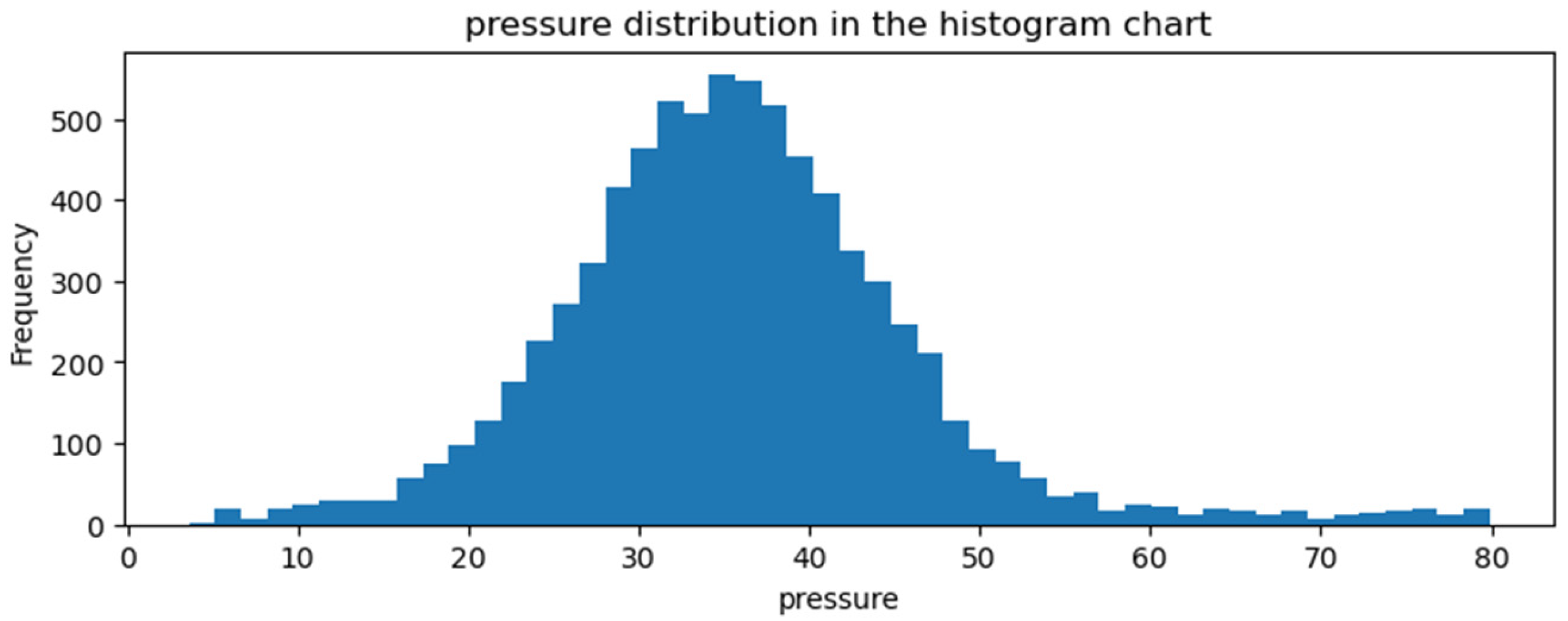
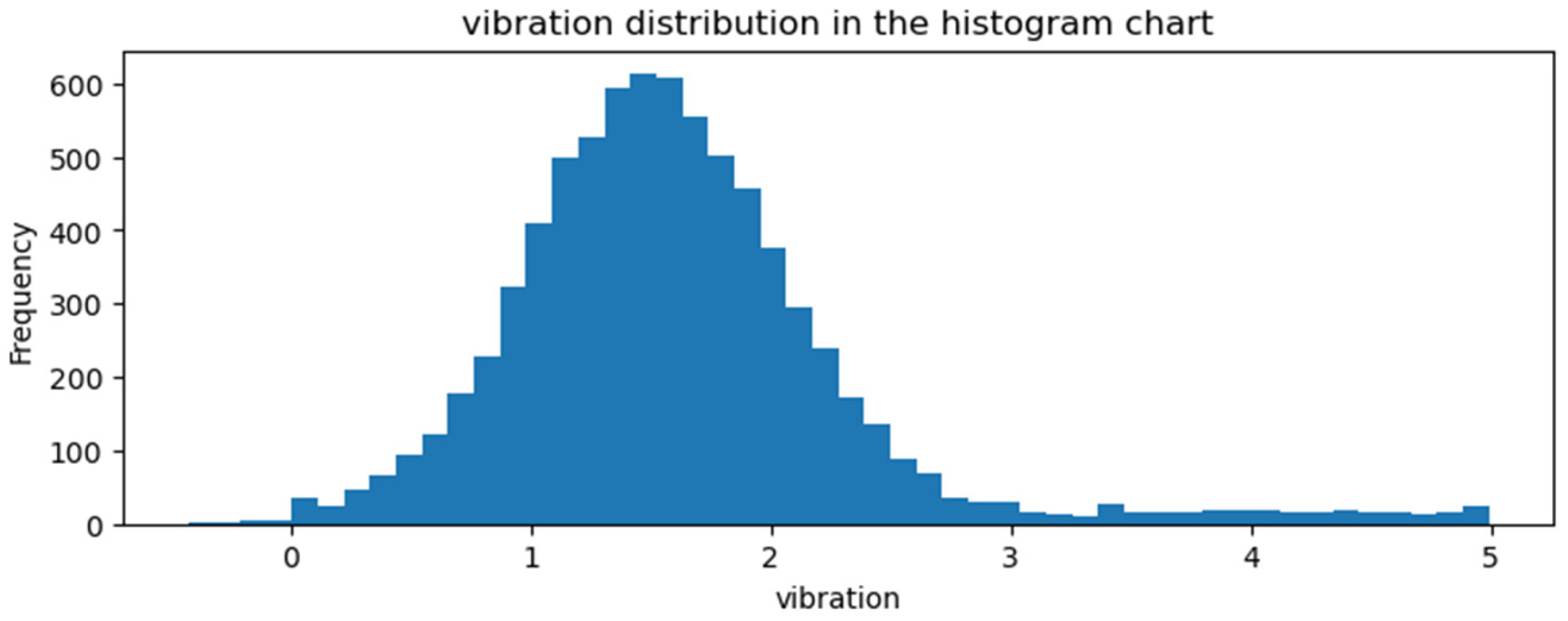
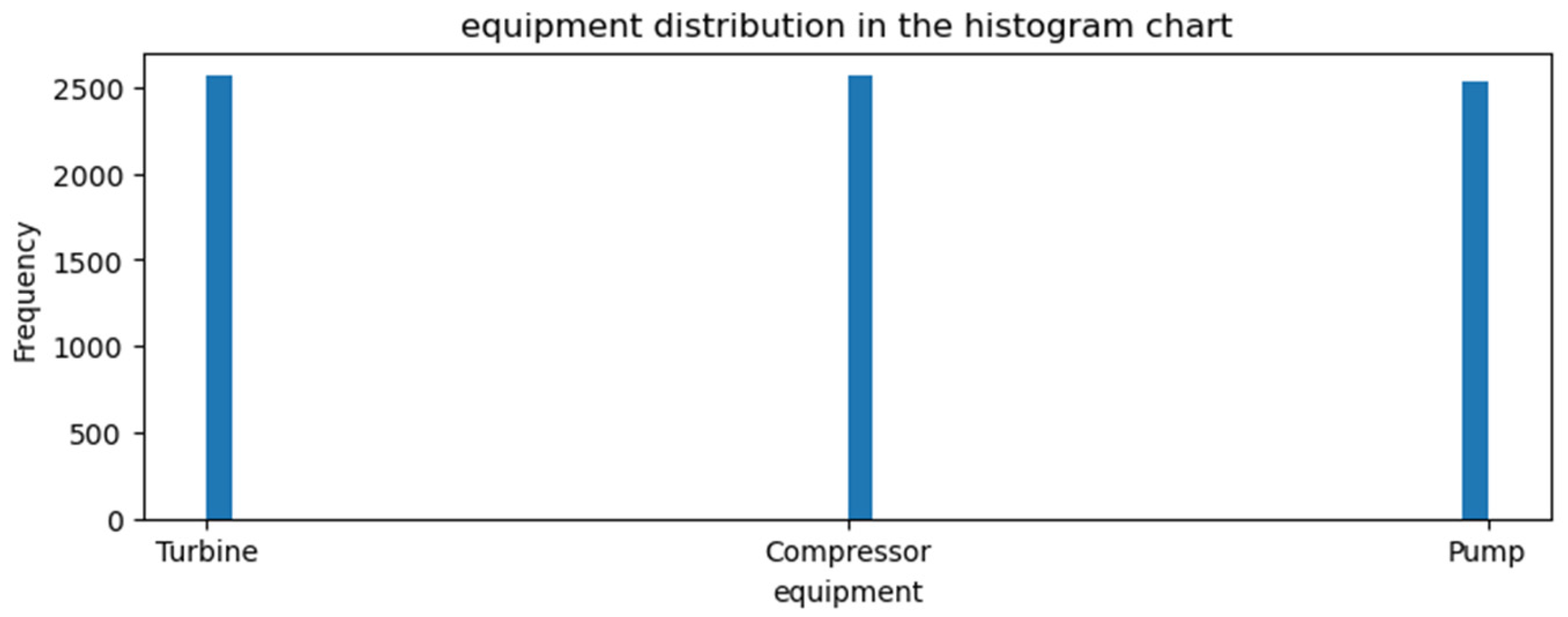
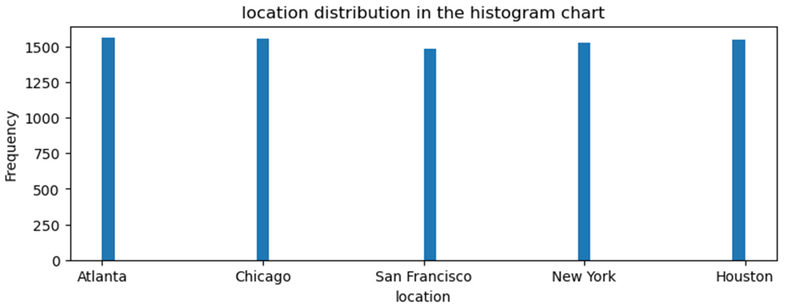
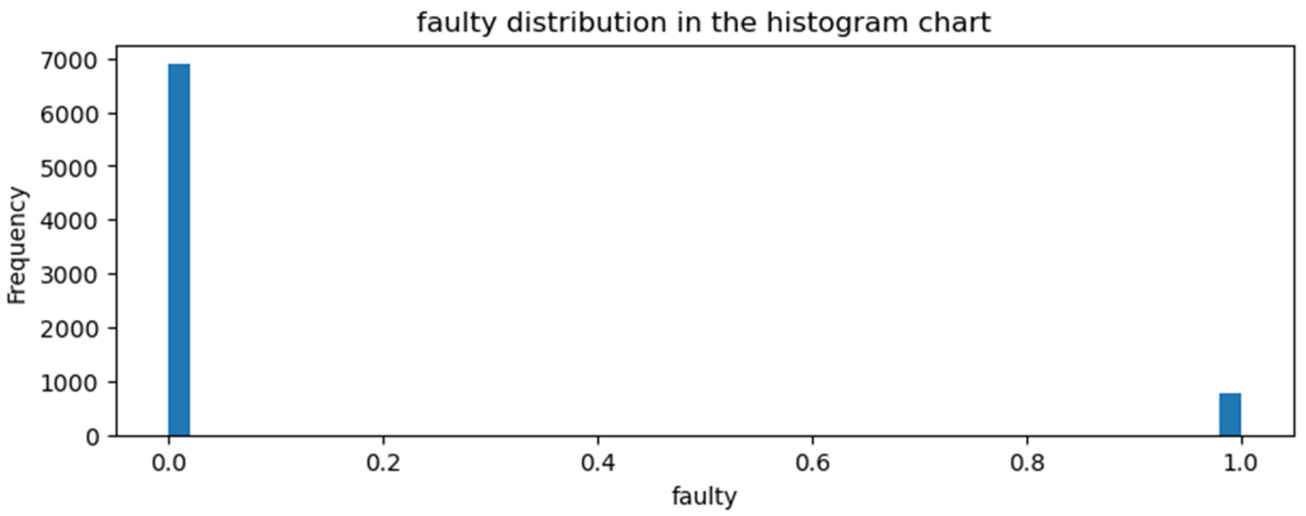
In this study, we used the Industrial Equipment Monitoring dataset provided by the Kaggle platform [18]. This dataset shared in the “https://www.kaggle.com/datasets/dnkumars/industrial-equipment-monitoring-dataset” link, released under the Apache 2.0 License (accessed on 1 August 2025). It consists of data that simulates real-time monitoring of various industrial equipment. Features of the dataset are temperature, pressure, vibration, humidity, equipment type, location, and equipment malfunction status. Temperature describes the temperature measurement in °C at the time of observation. Pressure defines the pressure measurement as bar at the moment of observation. Vibration is a measurement of vibration level. Humidity is the percentage of moisture. Equipment is the type of equipment. Location is the location of the equipment. Faulty describes the equipment’s operating status or the need for maintenance. Categories 0 and 1 define faultless and faulty states, respectively. The total number of data points is 7672. There is no missing data. A depiction of these features that create the dataset is provided in Figure 1, Figure 2, Figure 3, Figure 4, Figure 5, Figure 6 and Figure 7.

The temperature, pressure, vibration and humidity parameters given in Figure 1 are of float type and consist of 7672 unique values. Equipment and location parameters are object type. Data İn the equipment category includes compressor, turbine and pump features. The number of compressor data is 2573. The number of turbine data is 2565. The number of pump data is 2534. Data in the location category includes Atlanta, Chicago, Houston, New York, and San Francisco. The number of data points for Atlanta is 1564. The number of data points for Chicago is 1553. The number of data points for Houston is 1548. The number of data points for New York is 152. The number of data points for San Francisco is 1481. The number of 0.0 features in the Faulty category is 6905. The number of 1.0 features in the Faulty category is 767. These values show that the data distribution of the “faulty category”, data that defines the detection process is unbalanced. However, this dataset was selected because there is a need to develop new methods or improve existing methods to cope with unbalanced datasets in fault detection [4]. In total, 70% of the entire dataset is divided into training dataset and 30% is divided into testing data.

The industrial equipment monitoring dataset consists of simulated data for fault detection of various equipment. However, it is important to test the usability of the improved system in real-world scenarios. Therefore, the ReneWind dataset was used. This dataset shared in the “https://www.kaggle.com/datasets/mariyamalshatta/renewind” link is shared by the Kaggle platform under the CC0: Public Domain license (accessed on 20 August 2025). Its main focus is on renewable wind energy, which plays an important role in the global energy mix. It aims to improve machinery/processes in wind energy production. For this dataset, ReneWind company shared encrypted data on wind turbine generator failures obtained through sensors. The training and test datasets contain 20,000 and 5000 observations, respectively. Among the target variables, “1” is in the “fault present” category and “0” is in the “no fault present” category. There are 23,608 different observations in the “fault present” category. There are 1392 different data points in the “no fault present” category. Furthermore, this dataset consists of 40 predictor variables and 1 target variable. Predictor variables V1 and V2 contain 23 and 24 missing values, respectively, while the other predictor variables do not contain missing values. It is planned to build a strong model by sharing the dataset. The model to be improved aims to detect generator malfunctions before they break down. This will reduce costs. During the model improvement process, it is important to remove observations with missing data from the dataset. For this, a data cleaning process was implemented. With this process, missing values were deleted from the dataset.

In this study, the Iwo-Based Ann Algorithm that is initialized with fractal-based weights was applied to the ReneWind dataset. After data cleaning, 23,561 of the 24,953 remaining data points are in the “no fault” category, and 1392 were in the “fault” category. The ReneWind dataset and the Industrial Equipment Monitoring dataset are unbalanced. No balancing was performed between categories by synthetic data generation approach. Thus, it was planned to address the need to develop new methods or improve existing methods aimed at dealing with unbalanced datasets in fault detection.

2.2. Preprocessing

In recent years, deep learning-based studies have been actively used in fault detection because they make it possible to obtain complex relationships from machine-related data [17]. In this regard, exploratory data analysis, a data analysis procedure, is used to reveal critical features in the data [19]. This makes it possible to analyze the key parameters and failure rate and then make changes that will positively impact the performance of the dataset.

In this study, outlier values in the dataset were first deleted. This process reduced the number of datasets from 7672 to 7538. Secondly, a step-by-step column analysis was conducted. In this analysis, the “Fault Status” column is in binary format and therefore unchanged. The “Equipment” column is in categorical format. One-hot encoding was applied to the equipment feature to perform numerical operations. On the other hand, the “Temperature” column takes values between 10 and 149. These values can dominate the model because they offer a wide range. Therefore, a standard scaler was applied to temperature feature. The values in the pressure column range from 3 to 79. Because these values could mislead the model, the standard scaler was applied to the pressure feature. The “Humidity” column values range from 10 to 89. Because of the wide distribution, the values were normalized with a standard scaler. Vibration takes values between 0 and 4. Under normal conditions, the range of values is small. However, all data was compressed between 0 and 1. Therefore, the values in the “Vibrations” column were also normalized with a standard scaler. Thirdly, in the exploratory data analysis, the location feature, which does not have a potential positive impact on the results, was removed from the dataset. In the final case, the shape of the dataset is (7538,8).

2.3. Optimization

Optimization improves solution quality for complex problems [20]. It is evaluated within two different frameworks: stochastic and deterministic [21]. This study uses the IWO (Invasive Weed Optimization) metaheuristic optimization algorithm. IWO, which incorporates randomness, is a stochastic optimization algorithm [20]. It adopts a swarm intelligence-based approach.

3. Iwo-Based Ann Algorithm

In the real world, weeds are highly dispersive organisms. They exhibit high tolerance to environmental and climatic variations. Their rapid spread format causes damage to crops in agricultural fields. However, the combination of this invasive behavior of weeds with fitness and randomness parameters makes it possible to use the potential for spreading in optimization problems. This usage is presented within the framework of the Invasive Weed Optimization algorithm. The IWO algorithm includes population initiation, reproduction, identification of new locations, competitive elimination, and termination [20]. These situations related to the IWO algorithm will be explained with the variables VarMin, VarMax, nPop0, nPop, Smin, Smax, n, sigma_initial, sigma_final and MaxIt.

• The first stage is population initialization. In this stage, the seed assigned to nPop0 is randomly distributed in the solution space.
• The second stage is reproduction, which allows plants to produce seeds. The mathematical expression for this stage is given in Equations (1) and (2).

  $${\mathrm{r}\mathrm{a}\mathrm{t}\mathrm{i}\mathrm{o}}_{\mathrm{i}}={\displaystyle \frac{{\mathrm{f}(\mathrm{p}}_{\mathrm{i}})-\mathrm{ }{\mathrm{f}}_{\mathrm{w}\mathrm{o}\mathrm{r}\mathrm{s}\mathrm{t}}}{{\mathrm{f}}_{\mathrm{b}\mathrm{e}\mathrm{s}\mathrm{t}}-{\mathrm{f}}_{\mathrm{w}\mathrm{o}\mathrm{r}\mathrm{s}\mathrm{t}}+\mathrm{Ꜫ}}}$$

  (1)

  $${\mathrm{S}(\mathrm{p}}_{\mathrm{i}})={[\mathrm{S}}_{\mathrm{m}\mathrm{i}\mathrm{n}}+\left({\mathrm{S}}_{\mathrm{m}\mathrm{a}\mathrm{x}}-{\mathrm{S}}_{\min }\right).{\mathrm{r}\mathrm{a}\mathrm{t}\mathrm{i}\mathrm{o}}_{\mathrm{i}}$$

  (2)

  In Equation (1), f(p_i) is the fitness value of individual p_i. f_worst is the worst cost value in the population. f_best is the best cost value in the population. Ꜫ is the constant 1 × 10⁻¹² used to control the error of division by 0. S_min in Equation (2) is the minimum number of seeds. S_max is the maximum number of seeds.
• The third stage is the determination of new locations for the produced child seeds. In this section, the generated child seeds are placed by adding the random deviation value multiplied by the sigma value to the position of the parent. The sigma value for the ith iteration is calculated using the mathematical expression given in Equation (3).

  $${\mathsf{\sigma }}^{\left(\mathrm{i}\right)}={\left({\displaystyle \frac{\mathrm{M}\mathrm{a}\mathrm{x}\mathrm{I}\mathrm{t}-\mathrm{i}}{\mathrm{M}\mathrm{a}\mathrm{x}\mathrm{I}\mathrm{t}-1}}\right)}^{\mathrm{n}}.\left({\mathsf{\sigma }}_{\mathrm{i}\mathrm{n}\mathrm{i}\mathrm{t}\mathrm{i}\mathrm{a}\mathrm{l}}-{\mathsf{\sigma }}_{\mathrm{f}\mathrm{i}\mathrm{n}\mathrm{a}\mathrm{l}}\right)+{\mathsf{\sigma }}_{\mathrm{f}\mathrm{i}\mathrm{n}\mathrm{a}\mathrm{l}}$$

  (3)

  MaxIt, σ_initial and σ_final variables are used to calculate the sigma value within the scope of the i’th iteration in Equation (3). MaxIt is the total number of iterations. n is the rate of change in the sigma variable. sigma_initial and sigma_final are used to spread the seeds over a large space and then narrow down this space.
• The fourth stage is elimination. In this stage, the lowest-cost seeds are selected.
• The fifth stage is termination. Model training is completed when the MaxIt iteration count is reached.

The IWO mechanism operates for a specified number of iterations to optimize the bias and weight values of the artificial neural network model. The pseudocode of the ANN-based IWO optimization algorithm is given in Code 1.

Code 1.

1-The Industrial Equipment Monitoring dataset is given as input to the artificial neural network mechanism.  2-Predictions are obtained as a result of training using the feedforward process with the ANN mechanism.  3-The error value is calculated by comparing the actual and predicted values. This error value is then propagated back to the feedback layers.  4-The weight values are updated when the backpropagated gradient information is calculated. However, unlike the classical gradient descent method, IWO optimization is used for the update.  5-IWO optimization is an algorithm based on swarm intelligence. It focuses on finding the best combination of weight and bias parameters to be updated.

The 5 basic steps given in Code 1 ensure successful error detection. But it is possible to prevent getting stuck in local minima with a chaotic search. For this purpose, the metaheuristic optimization algorithm is designed to initialize with fractal-based weights. Thus, it aims to increase the power of global searches. For this, the initial population for the IWO algorithm is initialized with fractal-based values with different z values derived from the Julia set instead of random values. Detailed information about the Julia set is given below.

4. Julia Set

Dynamical systems are one-dimensional and two-dimensional. Two-dimensional systems have the potential to exhibit rich and complex behavior as a result of the differentiation of orbits that begin close together. In these dynamical systems, Julia sets of complex functions have been studied in the context of chaotic dynamics [22].

We consider the system F(z) = z². In this mathematical expression, z is a complex number. In this mathematical expression, z = x + iy. The i is the imaginary unit. The x and y are real numbers [22]. When the case given in Equation (4) is examined,

∣F(z₀)∣ = ∣z₀²∣ = ∣z₀∣² < ∣z₀∣

(4)

For ∣z0∣ < 1, the orbit of all valid points goes to 0. On the other hand, the orbit of points that provide the ∣z0∣ > 1 condition goes to infinity. These states are stable regions in the complex plane. On the other hand, there is also an unstable region. This region corresponds to the condition |z₀| = 1 on the unit circle. This region exhibiting chaotic behavior is called the Julia set. There are different methods for finding a Julia set. The first method is an inverse iteration method. At each step, as we move backward from the relevant point, the square root has either a positive or a negative root. This allows multiple paths to be generated. Any chosen path corresponds to a point in the Julia set. The second method is boundary scanning. Under the iteration of the F function, all points that do not go to infinity are drawn [22].

In this study, the code fragment [22] in BASIC programming language that draws the Julia set for functions in the form F(z) = z² + c using the reverse iteration method was translated into Python language. Then, the initial population for the IWO algorithm was initialized by fractal-based values with different z values derived from the Julia set, instead of random values. A chaotic and systematic distribution is structured with these values that constitute the initial population.

5. Results and Discussion

This study involves three main stages to maximize the final result. The first stage is preprocessing, which allows for the editing, addition, or removal of features that affect performance. The second stage is providing the prepared dataset as input to the IWO-based artificial neural network model. This stage optimizes the weight and bias values used in the artificial neural network approach using the IWO metaheuristic optimization algorithm. The third stage is initializing the initial weights with fractal-based weights instead of random initialization. But all of these stages have the potential to improve performance if appropriate parameters are selected. Therefore, 11 different experiments were conducted to test the artificial neural network model with different layer numbers. The layer numbers and the number of neurons used in these experiments were given in

Table 1. Parameter values for the experiments.

	Number of Layers	Number of Neurons Used in Each Layer
Experiment 1	1	5
Experiment 2	1	20
Experiment 3	1	40
Experiment 4	1	60
Experiment 5	2	10 20
Experiment 6	2	20 40
Experiment 7	3	10 30 50
Experiment 8	3	10 20 10
Experiment 9	3	20 40 20
Experiment 10	4	20 40 60 80
Experiment 11	5	10 20 30 40 50

. To determine the optimal number of layers for the planned target in the first stage, the parameters of the IWO optimization algorithm were not changed. These parameters were chosen as VarMin = −1, VarMax = 1, nPop0 = 10, nPop = 40, Smin = 0, Smax = 10, n = 1, sigma_initial = 1, sigma_final = 0.0001.

The experimental sets given in Table 1 were applied for 1000 iterations. Maximum success was achieved for Experiment 6, which had two hidden layers of 20 and 40 neurons on the training and test datasets, respectively. Fine tuning for the selection of the number of layers and the number of neurons increased the success. Therefore, the parameters of the IWO optimization algorithm will be modified along this layer hierarchy for subsequent architectures. Five different experiments were conducted for the fine tuning process of the parameters of the IWO optimization algorithm. These experiments are described below.

The 12th experiment is the retraining of the model in Experiment 6, which achieved the highest success with nPop0 = 10 and nPop = 40, for 1000 iterations with nPop0 = 10 and nPop = 60.

The 13th experiment is the retraining of the model in Experiment 6, which provided the highest success with Smin = 0 and Smax = 10, for 1000 iterations with Smin = 5 and Smax = 15 assignments.

The 14th experiment is a retraining of the model in Experiment 6, which achieved the highest success with n = 1 (n indicates that the number of seeds varies depending on the iterations) for 1000 iterations at n = 1.5. Another difference from the model hyperparameters trained in Experiment 6 is the assignment of Smin = 5 and Smax = 15, which optimized success in the thirteenth experiment.

Experiment 15 is the retraining of the model in Experiment 6, which achieved the highest success with sigma_initial = 1 and sigma_final = 0.0001, for 1000 iterations with sigma_initial = 1.5, sigma_final = 0.007.

The parameters related to the artificial neural network architecture of Experiment 6, which showed maximum performance, were kept constant for Experiment 12 - Experiment 15. However, the parameters related to the IWO optimization algorithm were adjusted. Accordingly, Experiment 16 was retrained for 1000 iterations with the hyperparameters VarMin = −1, VarMax = 1, nPop0 = 10, nPop = 50, Smin = 5, Smax = 15, n = 1.5, sigma_initial = 1.5, sigma_final = 0.0001. The achieved performance metrics are given in

Table 2. Performance metrics obtained over 1000 iterations for experiment 16.

	TP	FP	FN	TN	Accuracy	Weighted Precision	Weighted Recall	Weighted F1 Score
Training Dataset	4802	10	92	373	0.9807	0.9806	0.9807	0.9798
Testing Dataset	2087	6	36	132	0.9814	0.9811	0.9814	0.9806

.

The performance metrics given in Table 2 show the maximum performance achieved for experiment 16. The performance improvement in this experiment is explained by the fine-tuning of the neural network architecture and the IWO algorithm used to optimize the weights and biases of the neural network architecture. Compared to the architecture trained without tuning its parameters, performance improved by approximately 4%. This increase is significant because the model saturates at accuracies above 95%. Therefore, even a 1% increase represents a gain and indicates an increase in the model’s power by reducing the number of false positives.

All these experiments present a study to obtain appropriate values for the artificial neural network model and the IWO optimization algorithm. The summary of the selected values for Experiment 16, which shows maximum performance, is as follows. Two separate hidden layers were used in the artificial neural network architecture. The number of neurons in these hidden layers is 20 and 40, respectively. The hyperbolic tangent function was used in the hidden layers. In order to find appropriate weight and bias values during the training process of the artificial neural network architecture, the values of the integrated IWO optimization algorithm parameters VarMin, VarMax, MaxIt, nPop0, nPop, Smin, Smax, n, sigma_initial, sigma_final were determined as −1, 1, 1000, 10, 50, 5, 15, 1.5, 1.5, and 0.0001, respectively. Experiments ran for 1000 iterations. Under normal conditions, increasing the number of iterations indicates the model’s potential to obtain a better solution. But, if the solution does not improve, it is necessary to terminate the iteration. Therefore, Experiment 16, running 1000 iterations, was retrained for 2000, 3000, and 4000 iterations. A gradual performance increase was observed at 1000, 2000, and 3000 iterations. However, this increase was prevented by the 4000 iteration value. The model’s performance outputs for 3000 iterations are given in

Table 3. Performance metrics obtained for 3000 iterations within the scope of the fine-tuned model with maximum performance.

	TP	FP	FN	TN	Accuracy	Weighted Precision	Weighted Recall	Weighted F1 Score
Training Dataset	4806	6	72	393	0.9852	0.9852	0.9852	0.9847
Testing Dataset	2083	10	25	143	0.9845	0.9842	0.9845	0.9842

.

Table 3 shows the maximum performance with a 3000 iteration value. Therefore, 3000 iteration value was used in subsequent experiments.

The IWO-based ANN algorithm used in this study adopts a randomly assigned approach for the initial population. However, to improve solution quality, the IWO initial population was initialized with fractal-based values derived from the Julia Set. For functions of the form F(z) = z² + c, the different z values that constitute the Julie Set are the starting points.

In the IWO algorithm, weight assignment is initialized on z values for this study. The hyperparameters of experiment 16, which demonstrated maximum performance, were tested for 500 iterations at different z values. In this direction, the accuracy rates of 0.9748, 0.9699, 0.9766, 0.9783, 0.9726, 0.9779, 0.9752, 0.9713, 0.9730 were obtained in the test dataset for the values 0.1 + 0.1j, −2 − 2j, 2 − 2j, 2 + 2j, −0.8 + 0.156j, −0.4 + 0.6j, 0.285 + 0j, −0.70176 − 0.3842j, −0.1 + 0.651j, respectively. Accuracy rates of 0.9735, 0.9691, 0.9774, 0.9738, 0.9729, 0.9725, 0.9733, 0.9733, 0.9684 were obtained in the training datasets, respectively.

When examining the experiments, the value 2 − 2j assigned to z was chosen because the difference between the training and test datasets is small. This indicates the model’s stronger generalization ability. In addition to the balance in the training and test accuracy rates, the success rate for the training set is higher than for the test dataset. This indicates that the model is more reliable for real-world scenarios. The evaluation results achieved on the training and testing datasets by the 2 − 2j assignment for 3000 iterations are given in

Table 4. Performance metrics obtained by the 2 − 2j assignment for 3000 iterations.

2 − 2j	TP	FP	FN	TN	Accuracy	Weighted Precision	Weighted Recall	Weighted F1 Score
Training Dataset	4801	11	70	395	0.9847	0.9845	0.9847	0.9842
Testing Dataset	2083	10	21	147	0.9863	0.9860	0.9863	0.9861

.

When Table 4 is examined, the fractal evolution of z initialized with 2 − 2j exhibited a behavior that improved the true positive and true negative detection rate for the test dataset that the model has never seen.

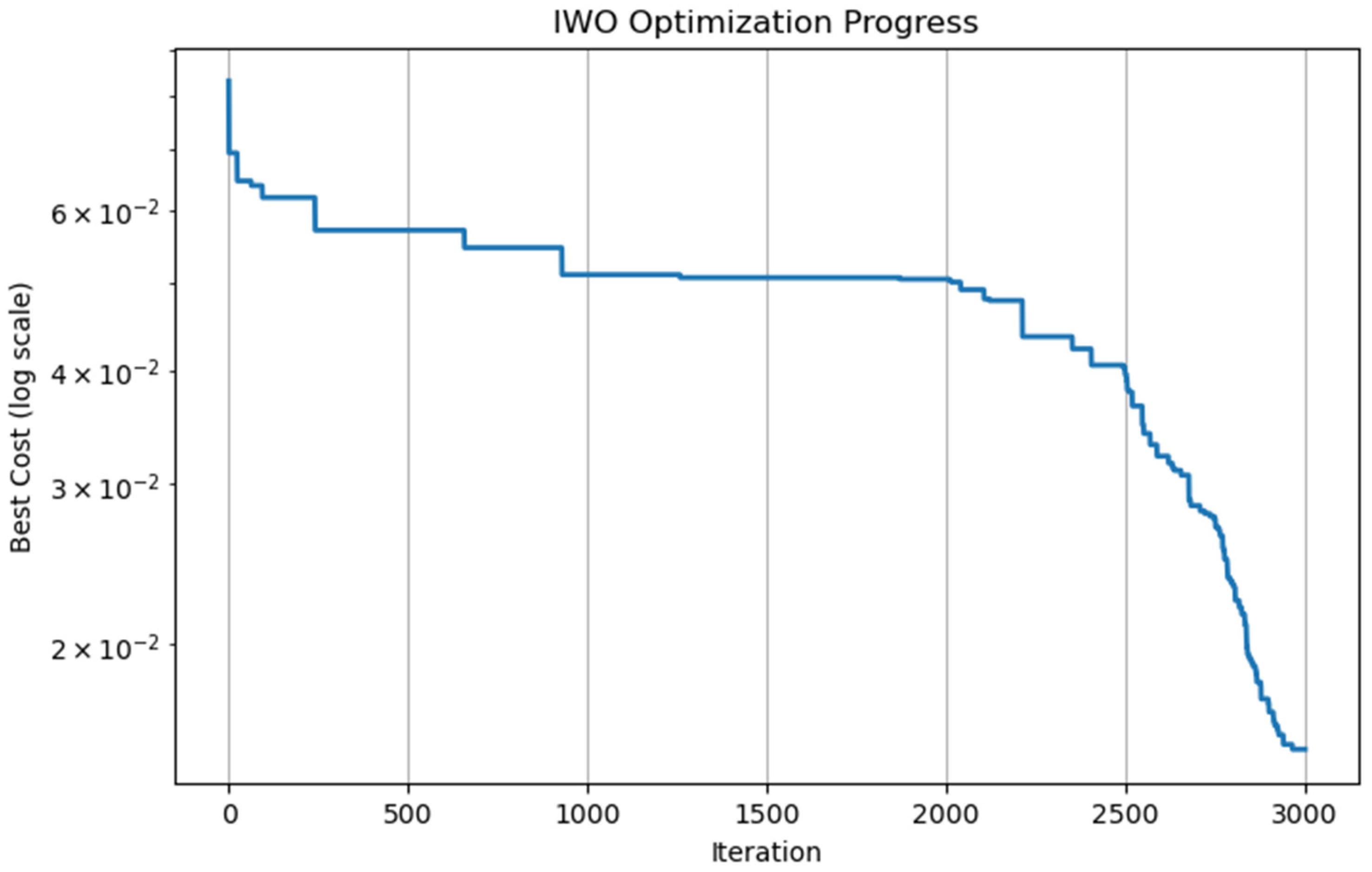
The cost related to the optimization process is given in Figure 8.

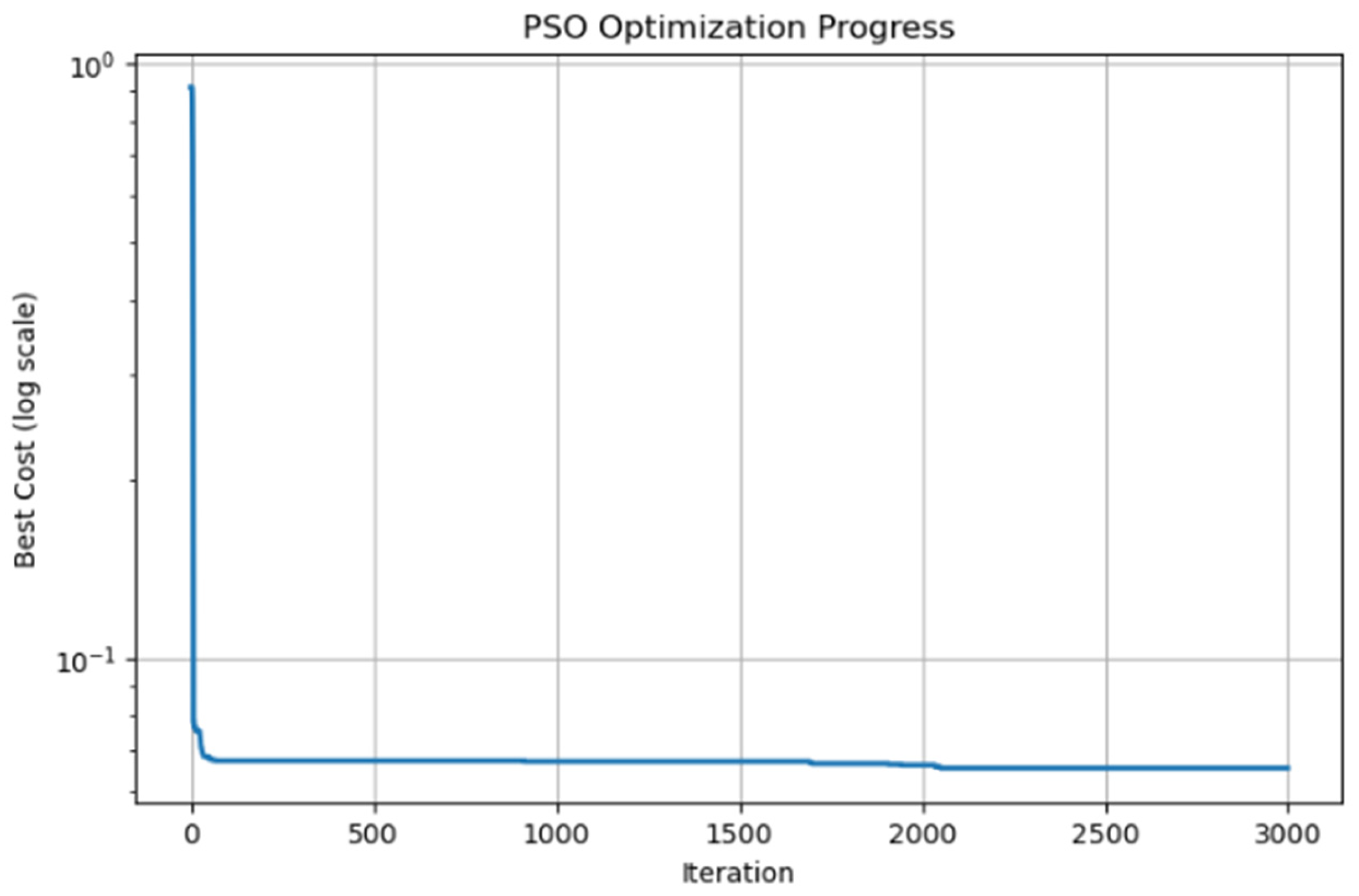
The IWO optimization algorithm whose cost analysis is performed in Figure 8 was initialized with fractal-based weights. But randomness was not removed in the new offspring generation. When the graph in Figure 8 is examined based on this information, it is seen that the rate of incorrect predictions in training gradually decreases throughout the iterations. Minimizing the cost as a result of this reduction indicates the success of the model. However, comparing the cost analysis of the improved model is another important issue. In this direction, the ANN based IWO optimization algorithm initialized with fractal-based weights was compared with the ANN based PSO algorithm initialized with fractal-based weights and the ANN based ABC algorithm initialized with fractal-based weights. The costs of the optimization process of these two hybrid structures are given in Figure 9 and Figure 10.

The PSO optimization algorithm, whose cost analysis is performed in Figure 9, was initialized with fractal-based weights. However, randomness was not eliminated in the r1 and r2 assignments used in the velocity update. On the other hand, the ABC optimization algorithm, whose cost analysis is performed in Figure 10, was initialized with fractal-based weights. However, randomness was not eliminated in the updates of the employed bees, onlooker bees, and scout bees. When the graphs given in Figure 9 and Figure 10 are examined based on this information, it is seen that the cost does not decrease gradually throughout the iterations. In addition, the minimum best cost point shown in Figure 8 was not reached. This indicates that the ANN-based IWO optimization algorithm initialized with fractal-based weights has a higher performance.

The concept of fractal used in this system is complex and unlimited forms. The field of study that examines these forms offers solutions to dynamic systems in the complex mathematical plane. Fractals are produced when even the simplest mathematical expressions are interpreted as dynamical systems. Furthermore, the fact that these fractals are generated by simple systems like z² + c makes them accessible and applicable to all disciplines [22].

In normal conditions, initializing the artificial neural network with random weights ensures that each neuron in the artificial neural network is unique. Thus learning and feature extraction capabilities improves. But this randomness lacks order. Performance fluctuates for repeated training. A poor start with the same architecture and hyperparameters can result in the model positioned directly in a shallow domain. It is possible that the model will get stuck in this area. This situation negatively affects the performance achieved throughout the training process. On the other hand, stability, consistency, and the ability to generalize are crucial for real-world scenarios. It prevents the process from being interrupted and ensures direct achievement of the goal, because it is important to combine the weights in an order. It eliminates the drawbacks of random initialization. Therefore, the fractal-based initialization used in this study is an important part of the optimization process, as it keeps the overall success and stability within a certain framework. The existence of real-life scenarios in a dynamic order confirms the necessity of this system. Also, the generalizability of the improved system is crucial. It should be tested on real-life observations as well as simulated data. For this reason, this approach, which proved its success on simulated data by the Industrial Equipment Monitoring dataset, was re-run on the ReneWind dataset consisting of real data under the same conditions. The evaluation results achieved on the training and testing datasets are given in

Table 5. Performance metrics obtained by the 2 − 2j assignment for 3000 iterations on ReneWind dataset.

2 − 2j	TP	FP	FN	TN	Accuracy	Weighted Precision	Weighted Recall	Weighted F1 Score
Training Dataset	7067	4	64	365	0.9909	0.9909	0.9909	0.9906
Testing Dataset	16,468	64	223	745	0.9836	0.9830	0.9836	0.9829

.

Table 5 shows the performance results generated by the IWO-based ANN model initialized with the fractal-based value of 2 − 2j z value of the dataset named ReneWind, which consists of real observations. The training outputs achieved on the training and test datasets show that the false alarm rate is low. Furthermore, the true positive and true negative detection rates are high. These explanations indicate the generalizability of the developed hybrid structure. Additionally, the datasets used in this study (the Industrial Equipment Monitoring dataset and the ReneWind dataset) are unbalanced. In fact, it is difficult to complete the detection process with high accuracy on imbalanced datasets. Especially in fault detection, new methods must be developed or existing methods must be improved to cope with this difficulty. The improved approach plays a complementary role in this respect. In particular, strengthening the detection process before a fault occurs improves net profit. It has applicability because it addresses the need in real-world scenarios.

This study successfully demonstrates how the optimization process is implemented to improve performance. Future analyses of the optimization process with different fractal clusters are planned.

6. Conclusions

Metaheuristic optimization algorithms are crucial for optimizing performance. They are valuable for selecting optimal parameters. However, randomly assigning the initial population carries the risk of getting stuck in a local minimum. Initializing the population space with fractal-based weights offers the potential to minimize this risk. In this study, the IWO optimization algorithm, whose parameters were fine-tuned, was integrated into the artificial neural network architecture to obtain appropriate weight and bias values. The initial population was then initialized with fractal-based values derived from the Julia Set. Thus, a chaotic and systematic distribution was constructed.

References

1. Singh, V.; Gangsar, P.; Porwal, R.; Atulkar, A. Artificial intelligence application in fault diagnostics of rotating industrial machines: A state-of-the-art review. J. Intell. Manuf. 2021, 34, 931–960. [Google Scholar] [CrossRef]
2. Das, M.K.; Rangarajan, K. Performance Monitoring and Failure Prediction of Industrial Equipments using Artificial Intelligence and Machine Learning Methods: A Survey. In Proceedings of the 4th International Conference on Computing Methodologies and Communication, ICCMC 2020, Erode, India, 11–13 March 2020; pp. 595–602. [Google Scholar] [CrossRef]
3. Gherghina, I.-S.; Bizon, N. Detection, Prevention, and Monitoring Techniques for Industrial Equipment—A brief review. In Proceedings of the 16th International Conference on Electronics, Computers and Artificial Intelligence, ECAI 2024, Iasi, Romania, 27–28 June 2024. [Google Scholar] [CrossRef]
4. Leite, D.; Andrade, E.; Rativa, D.; Maciel, A.M.A. Fault Detection and Diagnosis in Industry 4.0: A Review on Challenges and Opportunities. Sensors 2024, 25, 60. [Google Scholar] [CrossRef] [PubMed]
5. Akalin, F. Genetik Algoritma Temelli Yeni Bir Sentetik Veri Üretme Yaklaşımının Geliştirilmesi. Fırat Üniversitesi Mühendislik Bilim. Derg. 2023, 35, 753–760. [Google Scholar] [CrossRef]
6. Liu, R.; Yang, B.; Zio, E.; Chen, X. Artificial intelligence for fault diagnosis of rotating machinery: A review. Mech. Syst. Signal Process. 2018, 108, 33–47. [Google Scholar] [CrossRef]
7. Brito, L.C.; Susto, G.A.; Brito, J.N.; Duarte, M.A.V. An explainable artificial intelligence approach for unsupervised fault detection and diagnosis in rotating machinery. Mech. Syst. Signal Process. 2022, 163, 108105. [Google Scholar] [CrossRef]
8. Mazzoleni, M.; Sarda, K.; Acernese, A.; Russo, L.; Manfredi, L.; Glielmo, L.; Del Vecchio, C. A fuzzy logic-based approach for fault diagnosis and condition monitoring of industry 4.0 manufacturing processes. Eng. Appl. Artif. Intell. 2022, 115, 105317. [Google Scholar] [CrossRef]
9. Shao, X.; Cai, B.; Zou, Z.; Shao, H.; Yang, C.; Liu, Y. Artificial intelligence enhanced fault prediction with industrial incomplete information. Mech. Syst. Signal Process. 2025, 224, 112063. [Google Scholar] [CrossRef]
10. Brusa, E.; Cibrario, L.; Delprete, C.; Di Maggio, L.G. Explainable AI for Machine Fault Diagnosis: Understanding Features’ Contribution in Machine Learning Models for Industrial Condition Monitoring. Appl. Sci. 2023, 13, 2038. [Google Scholar] [CrossRef]
11. Gültekin, Ö.; Cinar, E.; Özkan, K.; Yazıcı, A. Real-Time Fault Detection and Condition Monitoring for Industrial Autonomous Transfer Vehicles Utilizing Edge Artificial Intelligence. Sensors 2022, 22, 3208. [Google Scholar] [CrossRef] [PubMed]
12. Nyanteh, Y.; Edrington, C.; Srivastava, S.; Cartes, D. Application of artificial intelligence to real-time fault detection in permanent-magnet synchronous machines. IEEE Trans. Ind. Appl. 2013, 49, 1205–1214. [Google Scholar] [CrossRef]
13. Li, Z.; Kristoffersen, E.; Li, J. Deep transfer learning for failure prediction across failure types. Comput. Ind. Eng. 2022, 172, 108521. [Google Scholar] [CrossRef]
14. Hosseinzadeh, A.; Chen, F.F.; Shahin, M.; Bouzary, H. A predictive maintenance approach in manufacturing systems via AI-based early failure detection. Manuf. Lett. 2023, 35, 1179–1186. [Google Scholar] [CrossRef]
15. Wahid, A.; Breslin, J.G.; Intizar, M.A. Prediction of Machine Failure in Industry 4.0: A Hybrid CNN-LSTM Framework. Appl. Sci. 2022, 12, 4221. [Google Scholar] [CrossRef]
16. Eang, C.; Lee, S. Predictive Maintenance and Fault Detection for Motor Drive Control Systems in Industrial Robots Using CNN-RNN-Based Observers. Sensors 2025, 25, 25. [Google Scholar] [CrossRef] [PubMed]
17. Eldele, E.; Ragab, M.; Qing, X.; Edward; Chen, Z.; Wu, M.; Li, X.; Lee, J. UniFault: A Fault Diagnosis Foundation Model from Bearing Data. arXiv 2025, arXiv:2504.01373. [Google Scholar] [CrossRef]
18. Kaggle Datasets. Available online: https://www.kaggle.com/datasets (accessed on 20 August 2025).
19. Shabbir, A.; Shabbir, M.; Javed, A.R.; Rizwan, M.; Iwendi, C.; Chakraborty, C. Exploratory data analysis, classification, comparative analysis, case severity detection, and internet of things in COVID-19 telemonitoring for smart hospitals. J. Exp. Theor. Artif. Intell. 2022, 35, 507–534. [Google Scholar] [CrossRef]
20. Huang, L.; Asteris, P.G.; Koopialipoor, M.; Armaghani, D.J.; Tahir, M.M. Invasive weed optimization technique-based ANN to the prediction of rock tensile strength. Appl. Sci. 2019, 9, 5372. [Google Scholar] [CrossRef]
21. Akalın, F. Survival Classification in Heart Failure Patients by Neural Network-Based Crocodile and Egyptian Plover (CEP) Optimization Algorithm. Arab. J. Sci. Eng. 2023, 49, 3897–3914. [Google Scholar] [CrossRef]
22. Michael, F.; Barnsley Robert, L.; Devaney Benoit, B. Mandelbrot Heinz-Otto Peitgen Dietmar Saupe Richard F. Voss With Contributions by Yuval Fisher Michael McGuire. In The Science of Fractal Images; Springer: Berlin/Heidelberg, Germany, 1988. [Google Scholar]
Figure 1. Distribution of temperature values in the histogram chart.
Electronics 14 03403 g001
Figure 2. Distribution of pressure values in the histogram chart.
Electronics 14 03403 g002
Figure 3. Distribution of vibration values in the histogram chart.
Electronics 14 03403 g003
Figure 4. Distribution of humidity values in the histogram chart.
Electronics 14 03403 g004
Figure 5. Distribution of equipment categories in the histogram chart.
Electronics 14 03403 g005
Figure 6. Distribution of location categories in the histogram chart.
Electronics 14 03403 g006
Figure 7. Distribution of faulty categories in the histogram chart.
Electronics 14 03403 g007
Figure 8. Cost analysis of the ANN-based IWO optimization algorithm initialized with fractal-based weights over iterations.
Electronics 14 03403 g008
Figure 9. Cost analysis of the ANN-based PSO optimization algorithm initialized with fractal-based weights over iterations.
Electronics 14 03403 g009
Figure 10. Cost analysis of the ANN-based ABC optimization algorithm initialized with fractal-based weights over iterations.
Electronics 14 03403 g010