Figure 1.
Structural diagram of the WTCMC network: (a) data preprocessing, (b) SFE, (c) wavelet processing, (d) LFSM and HFMC, (e) SCF, and (f) classification head. The workflow involves initially reducing the dimensionality of the raw input image using principal component analysis (PCA), followed by partitioning the resultant image into multiple patches. These image patches first pass through the shallow feature extraction module and are subsequently upsampled via bilinear interpolation. Next, a wavelet transform is applied to decompose the upsampled patches into low-frequency and high-frequency subbands. The low-frequency subbands are processed by the low-frequency spectral Mamba module, while the high-frequency subbands are handled by the high-frequency multi-scale convolution module. Finally, features extracted from both modules are integrated through the spectral–spatial complementary fusion module. The resulting fused features are then classified by the classification head, which consists of average pooling and a normalized linear layer.
![Electronics 14 03301 g001 Electronics 14 03301 g001]()
Figure 2.
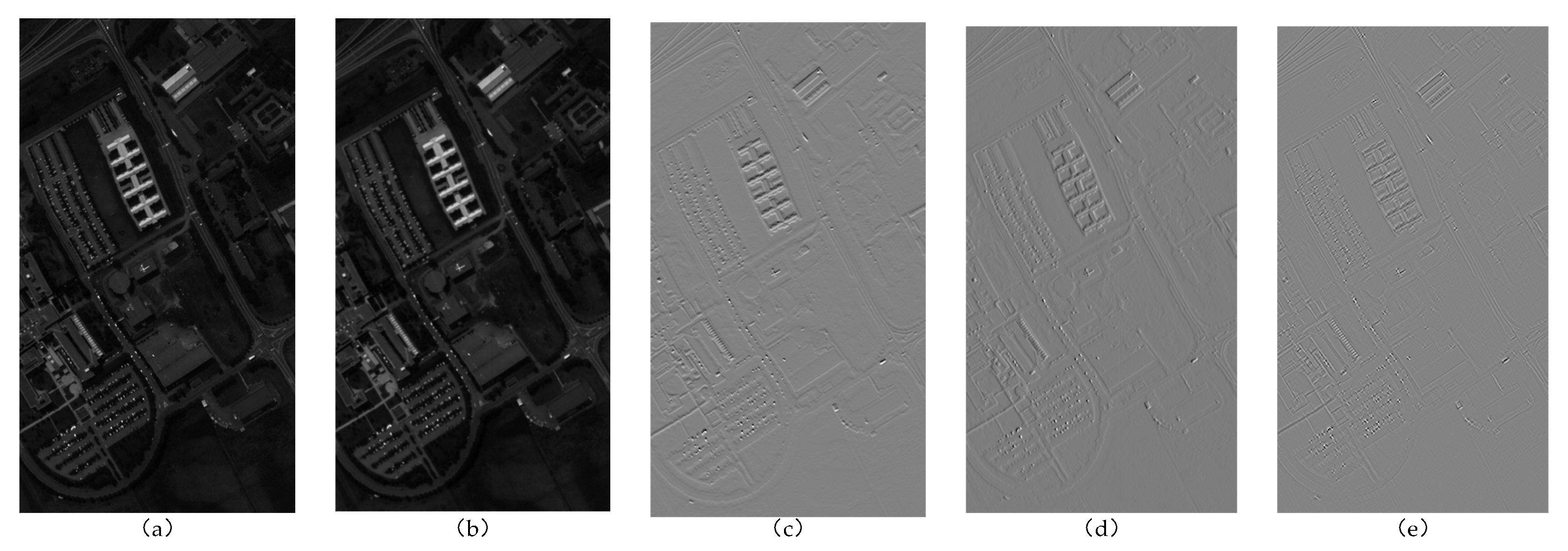
Schematic diagram of a band of the PU dataset before and after wavelet transform: (a) original image, (b) low-frequency subband , (c) high-frequency subband , (d) high-frequency subband , and (e) high-frequency subband .
Figure 2.
Schematic diagram of a band of the PU dataset before and after wavelet transform: (a) original image, (b) low-frequency subband , (c) high-frequency subband , (d) high-frequency subband , and (e) high-frequency subband .
Figure 3.
Structural diagram of the shallow feature extraction module.
Figure 3.
Structural diagram of the shallow feature extraction module.
Figure 4.
Structural diagram of the low-frequency spectral Mamba module.
Figure 4.
Structural diagram of the low-frequency spectral Mamba module.
Figure 5.
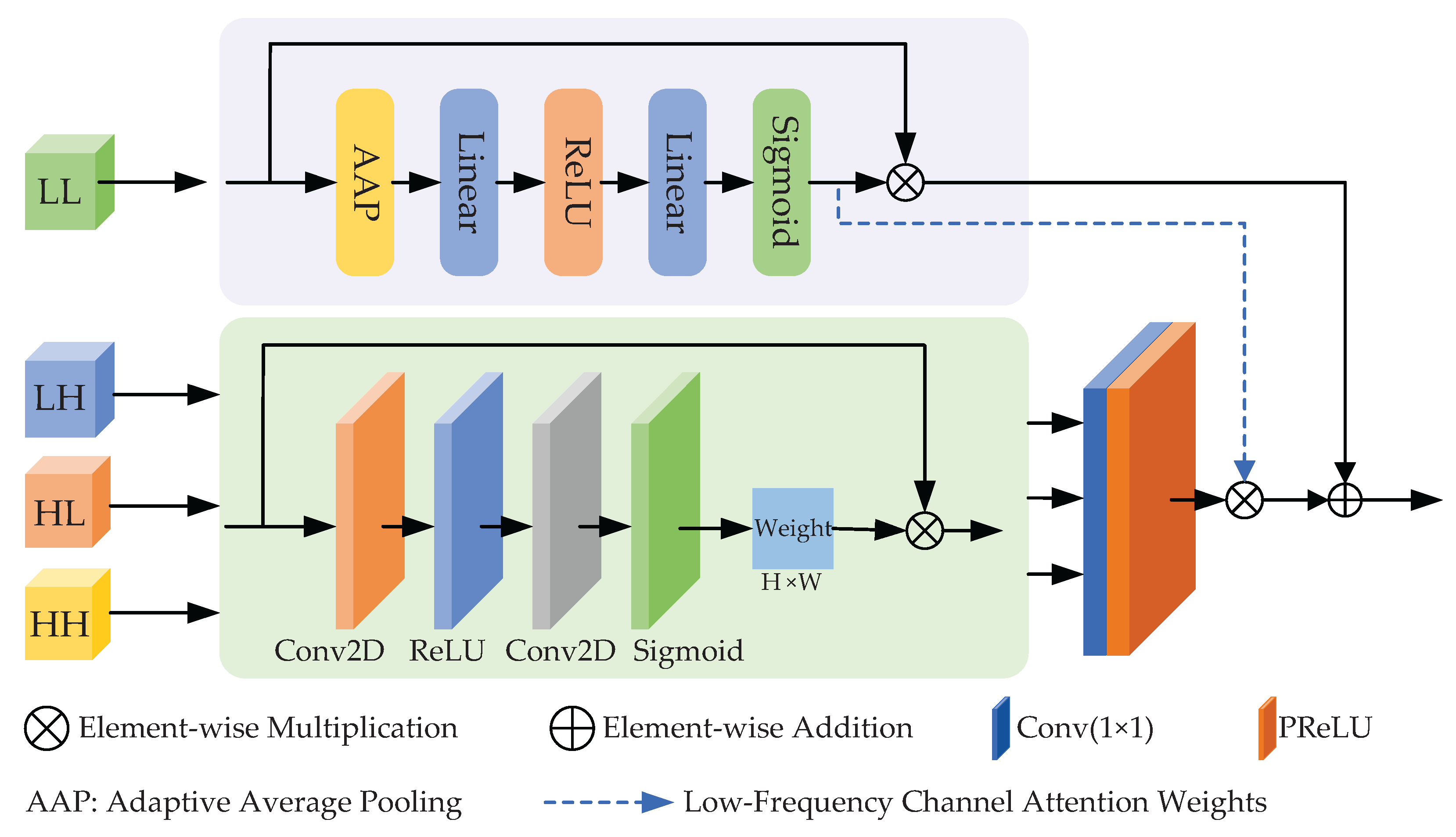
Structural diagram of the high-frequency multi-scale convolution module.
Figure 5.
Structural diagram of the high-frequency multi-scale convolution module.
Figure 6.
Structural diagram of the spectral–spatial complementary fusion module.
Figure 6.
Structural diagram of the spectral–spatial complementary fusion module.
Figure 7.
Pavia University dataset: (a) false color map and (b) ground truth.
Figure 7.
Pavia University dataset: (a) false color map and (b) ground truth.
Figure 8.
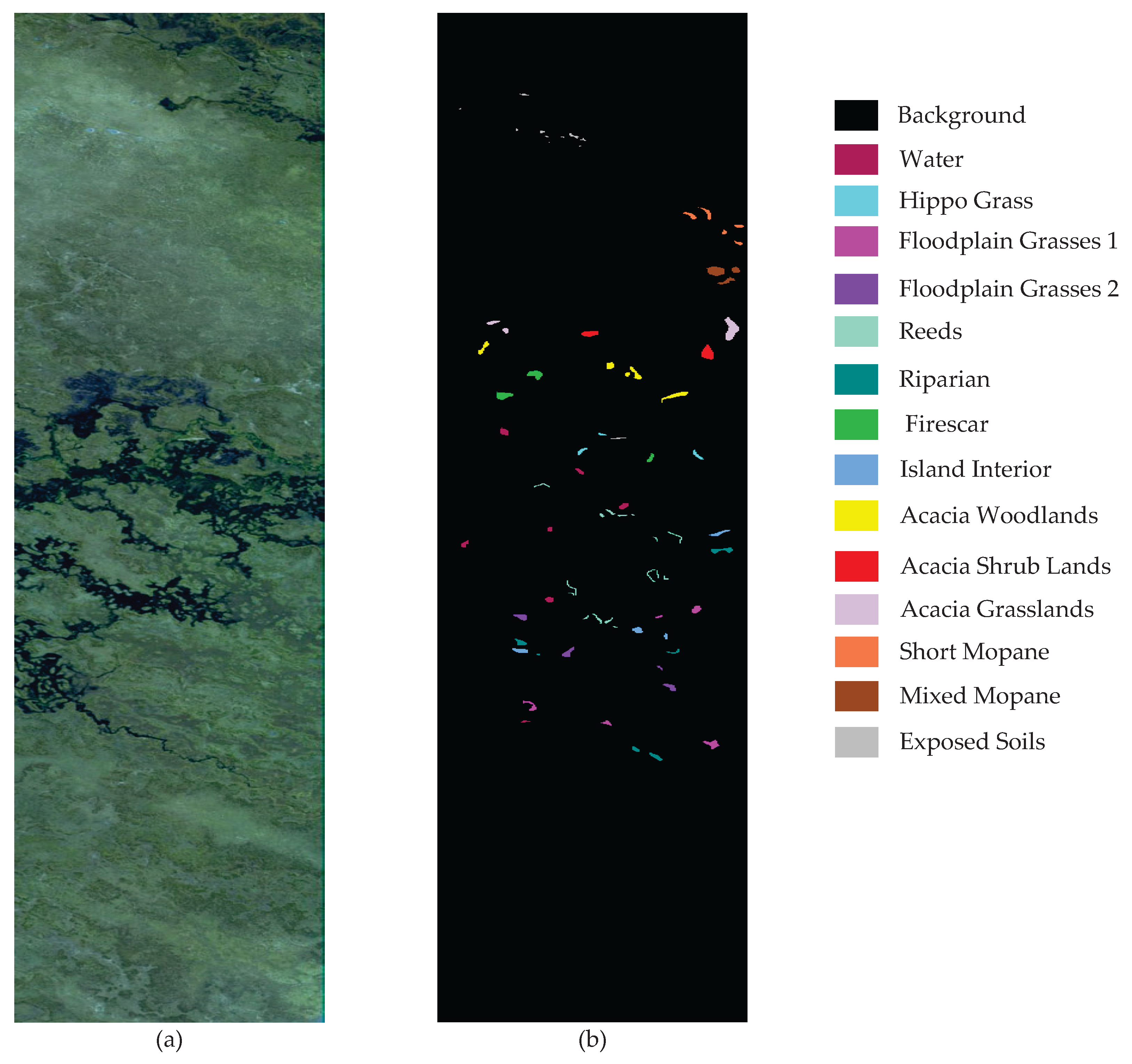
Botswana dataset: (a) false color map and (b) ground truth.
Figure 8.
Botswana dataset: (a) false color map and (b) ground truth.
Figure 9.
Indian Pines dataset: (a) false color map and (b) ground truth.
Figure 9.
Indian Pines dataset: (a) false color map and (b) ground truth.
Figure 10.
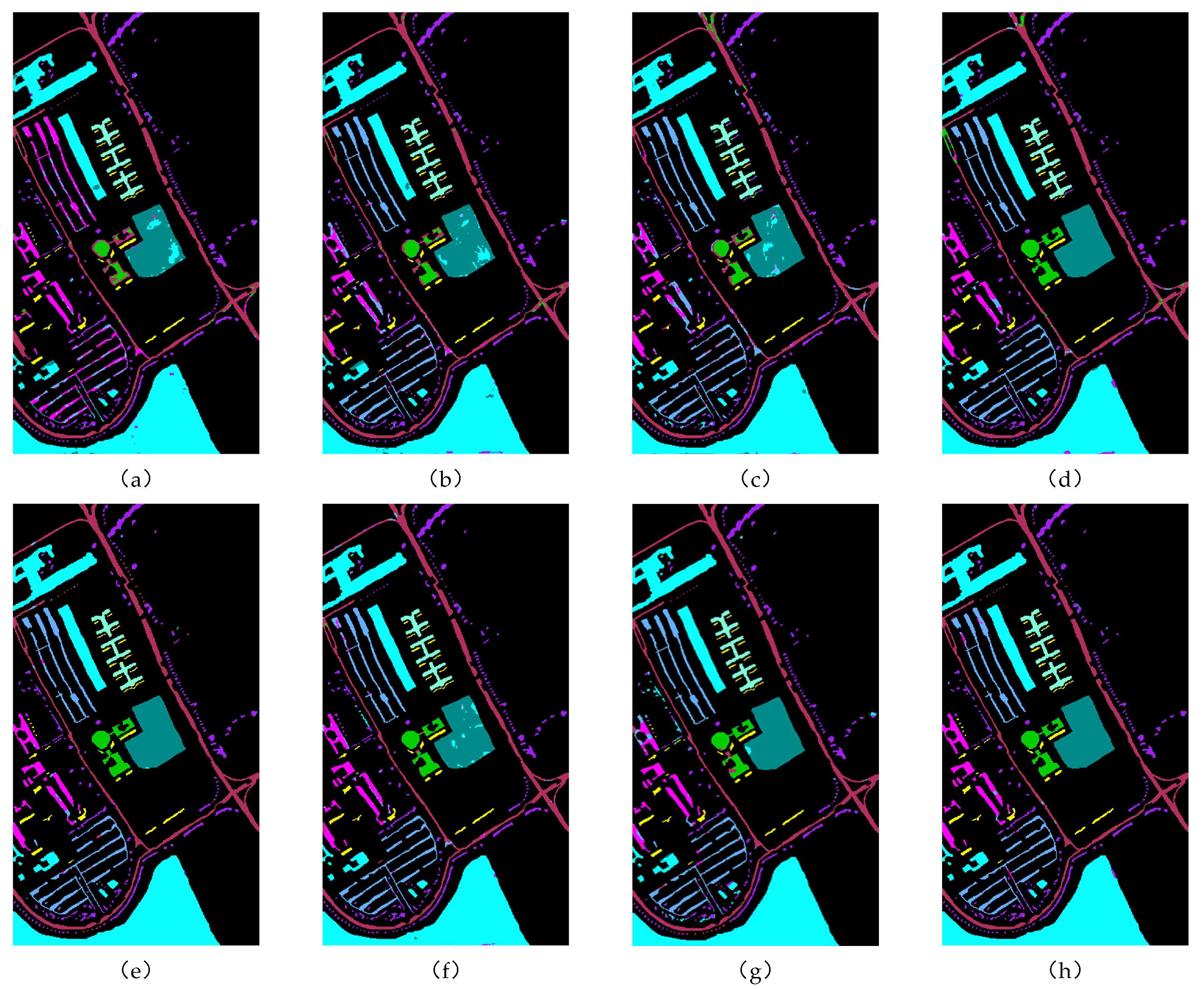
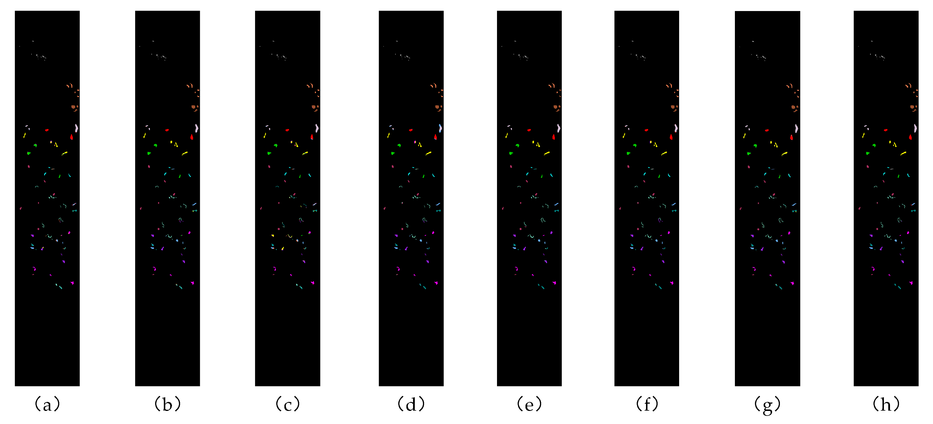
Classification effect diagram of all methods on the PU dataset: (a) 2DCNN, (b) 3DCNN, (c) SpectralFormer, (d) SSFTT, (e) MassFormer, (f) GSCVIT, (g) MambaHSI, and (h) WTCMC.
Figure 10.
Classification effect diagram of all methods on the PU dataset: (a) 2DCNN, (b) 3DCNN, (c) SpectralFormer, (d) SSFTT, (e) MassFormer, (f) GSCVIT, (g) MambaHSI, and (h) WTCMC.
Figure 11.
Classification effect diagram of all methods on the Botswana dataset: (a) 2DCNN, (b) 3DCNN, (c) SpectralFormer, (d) SSFTT, (e) MassFormer, (f) GSCVIT, (g) MambaHSI, and (h) WTCMC.
Figure 11.
Classification effect diagram of all methods on the Botswana dataset: (a) 2DCNN, (b) 3DCNN, (c) SpectralFormer, (d) SSFTT, (e) MassFormer, (f) GSCVIT, (g) MambaHSI, and (h) WTCMC.
Figure 12.
Classification effect diagram of all methods on the Indian Pines dataset: (a) 2DCNN, (b) 3DCNN, (c) SpectralFormer, (d) SSFTT, (e) MassFormer, (f) GSCVIT, (g) MambaHSI, and (h) WTCMC.
Figure 12.
Classification effect diagram of all methods on the Indian Pines dataset: (a) 2DCNN, (b) 3DCNN, (c) SpectralFormer, (d) SSFTT, (e) MassFormer, (f) GSCVIT, (g) MambaHSI, and (h) WTCMC.
Figure 13.
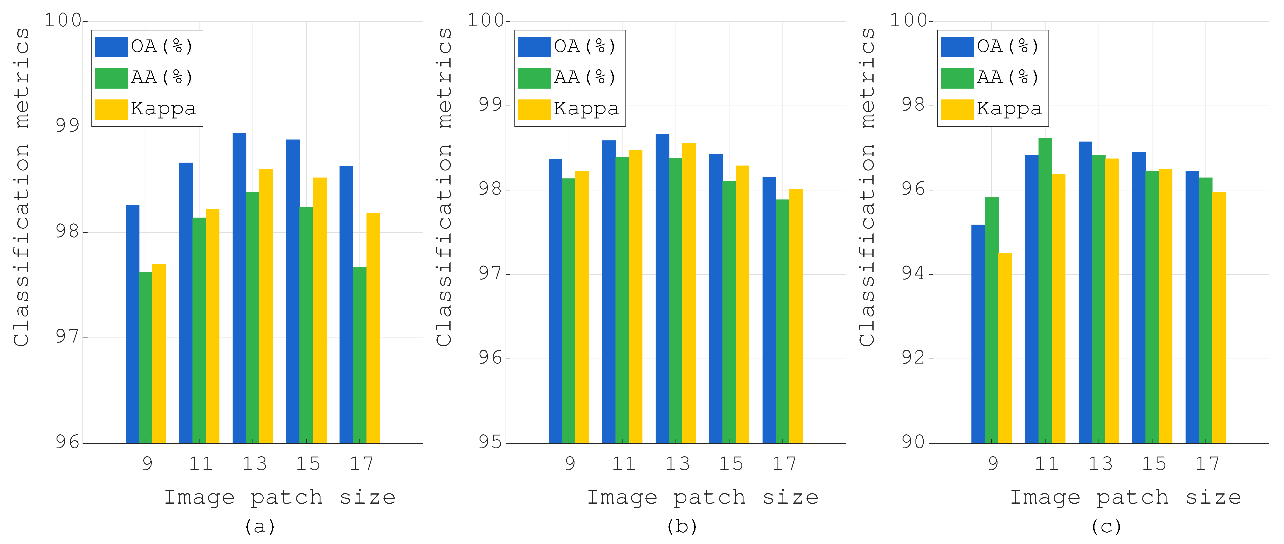
Effect of the image patch size on PU, Botswana, and IP datasets: (a) PU, (b) Botswana, and (c) IP.
Figure 13.
Effect of the image patch size on PU, Botswana, and IP datasets: (a) PU, (b) Botswana, and (c) IP.
Figure 14.
Effect of the number of bands after PCA on PU, Botswana, and IP datasets: (a) PU, (b) Botswana, and (c) IP.
Figure 14.
Effect of the number of bands after PCA on PU, Botswana, and IP datasets: (a) PU, (b) Botswana, and (c) IP.
Figure 15.
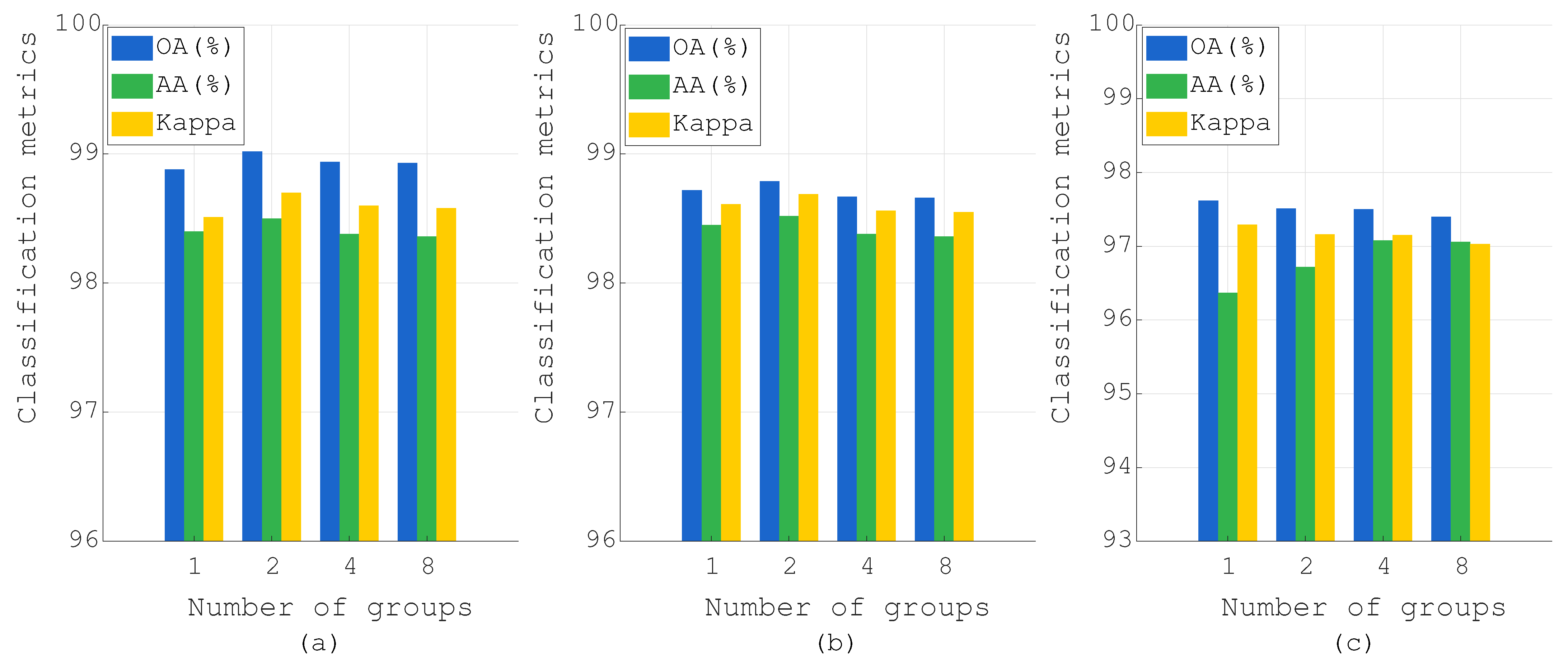
Effect of the number of groups in LFSM on PU, Botswana, and IP datasets: (a) PU, (b) Botswana, and (c) IP.
Figure 15.
Effect of the number of groups in LFSM on PU, Botswana, and IP datasets: (a) PU, (b) Botswana, and (c) IP.
Table 1.
Concise comparison of CNN-, transformer-, Mamba-, and wavelet-based methods versus WTCMC.
Table 1.
Concise comparison of CNN-, transformer-, Mamba-, and wavelet-based methods versus WTCMC.
| Methods | Structure | Frequency Domain | Multi-Scale Strategy | Attention Mechanism |
|---|
| [31,32,33] | CNN-based | Not supported | Partially supported | Partially supported |
| [21,22] | Transformer-based | Not supported | Partially supported | Supported |
| [34,35,36,37,38,39] | Mamba-based | Partially supported | Partially supported | Partially supported |
| [28,29,30] | Wavelet-based | Supported | supported | Partially supported |
| \ | WTCMC | Supported | Supported | Supported |
Table 2.
The number of samples in the training set, validation set, and test set of the Pavia University dataset.
Table 2.
The number of samples in the training set, validation set, and test set of the Pavia University dataset.
| No. | Class Name | Train | Val | Test | Total |
|---|
| 1 | Asphalt | 66 | 66 | 6499 | 6631 |
| 2 | Meadows | 186 | 186 | 18,277 | 18,649 |
| 3 | Gravel | 21 | 21 | 2057 | 2099 |
| 4 | Trees | 31 | 31 | 3002 | 3064 |
| 5 | Painted Metal Sheets | 13 | 13 | 1319 | 1345 |
| 6 | Bare Soil | 50 | 50 | 4929 | 5029 |
| 7 | Bitumen | 13 | 13 | 1304 | 1330 |
| 8 | Self-Blocking Bricks | 37 | 37 | 3608 | 3682 |
| 9 | Shadows | 10 | 10 | 927 | 947 |
| Total | 427 | 427 | 41,922 | 42,776 |
Table 3.
The number of samples in the training set, validation set, and test set of the Botswana dataset.
Table 3.
The number of samples in the training set, validation set, and test set of the Botswana dataset.
| No. | Class Name | Train | Val | Test | Total |
|---|
| 1 | Water | 8 | 8 | 254 | 270 |
| 2 | Hippo Grass | 3 | 3 | 95 | 101 |
| 3 | Floodplain Grasses 1 | 8 | 8 | 235 | 251 |
| 4 | Floodplain Grasses 2 | 7 | 6 | 202 | 215 |
| 5 | Reeds | 8 | 8 | 253 | 269 |
| 6 | Riparian | 8 | 8 | 253 | 269 |
| 7 | Firescar | 8 | 8 | 243 | 259 |
| 8 | Island Interior | 6 | 6 | 191 | 203 |
| 9 | Acacia Woodlands | 9 | 9 | 296 | 314 |
| 10 | Acacia Shrub Lands | 7 | 8 | 233 | 248 |
| 11 | Acacia Grasslands | 9 | 9 | 287 | 305 |
| 12 | Short Mopane | 5 | 5 | 171 | 181 |
| 13 | Mixed Mopane | 8 | 8 | 252 | 268 |
| 14 | Exposed Soils | 3 | 3 | 89 | 95 |
| Total | 97 | 97 | 3054 | 3248 |
Table 4.
The number of samples in the training set, validation set, and test set of the Indian Pines dataset (partial class name abbreviation).
Table 4.
The number of samples in the training set, validation set, and test set of the Indian Pines dataset (partial class name abbreviation).
| No. | Class Name | Train | Val | Test | Total |
|---|
| 1 | Alfalfa | 2 | 2 | 42 | 46 |
| 2 | Corn-notill | 71 | 71 | 1286 | 1428 |
| 3 | Corn-mintill | 41 | 42 | 747 | 830 |
| 4 | Corn | 12 | 12 | 213 | 237 |
| 5 | Grass-pasture | 24 | 24 | 435 | 483 |
| 6 | Grass-trees | 37 | 36 | 657 | 730 |
| 7 | Pasture-mowed | 1 | 1 | 26 | 28 |
| 8 | Hay-windrowed | 24 | 24 | 430 | 478 |
| 9 | Oats | 1 | 1 | 18 | 20 |
| 10 | Soybean-notill | 49 | 49 | 874 | 972 |
| 11 | Soybean-mintill | 123 | 123 | 2209 | 2455 |
| 12 | Soybean-clean | 30 | 30 | 533 | 593 |
| 13 | Wheat | 10 | 10 | 185 | 205 |
| 14 | Woods | 63 | 63 | 1139 | 1265 |
| 15 | Building-grass | 19 | 19 | 348 | 386 |
| 16 | Stone-steel-towers | 5 | 5 | 83 | 93 |
| Total | 512 | 512 | 9225 | 10,249 |
Table 5.
Classification results of different methods on Pavia University dataset (SpectralFormer is abbreviated as SpeFormer).
Table 5.
Classification results of different methods on Pavia University dataset (SpectralFormer is abbreviated as SpeFormer).
| Class | 2DCNN | 3DCNN | SpeFormer | SSFTT | MassFormer | GSCVIT | MambaHSI | WTCMC |
|---|
| 1 | 91.05 | 94.53 | 91.36 | 96.73 | 98.97 | 97.82 | 97.92 | 98.82 |
| 2 | 97.07 | 98.76 | 98.73 | 99.70 | 99.79 | 99.34 | 99.52 | 99.85 |
| 3 | 68.58 | 73.94 | 75.99 | 94.32 | 93.93 | 91.34 | 75.96 | 95.44 |
| 4 | 97.16 | 98.00 | 93.24 | 97.69 | 91.97 | 96.62 | 87.23 | 97.59 |
| 5 | 99.61 | 99.23 | 99.87 | 98.95 | 98.26 | 99.34 | 98.22 | 99.86 |
| 6 | 92.81 | 87.89 | 92.12 | 99.10 | 99.55 | 97.38 | 98.98 | 99.87 |
| 7 | 64.21 | 74.95 | 70.68 | 94.47 | 99.85 | 94.19 | 86.97 | 99.84 |
| 8 | 79.66 | 90.25 | 87.02 | 96.05 | 94.95 | 94.99 | 99.43 | 95.92 |
| 9 | 97.62 | 97.22 | 93.06 | 96.61 | 95.35 | 98.41 | 96.52 | 98.26 |
| OA (%) | 91.82 ± 3.04 | 94.06 ± 0.62 | 93.33 ± 0.58 | 98.19 ± 0.47 | 98.23 ± 0.20 | 97.78 ± 0.37 | 96.26 ± 0.68 | 98.94 ± 0.15 |
| AA (%) | 87.53 ± 5.40 | 90.53 ± 1.06 | 89.12 ± 1.37 | 97.07 ± 0.79 | 96.96 ± 0.29 | 96.65 ± 0.75 | 92.75 ± 1.25 | 98.38 ± 0.22 |
| Kappa | 89.17 ± 4.02 | 92.09 ± 0.85 | 91.13 ± 0.78 | 97.60 ± 0.62 | 97.65 ± 0.26 | 97.06 ± 0.49 | 95.26 ± 1.26 | 98.60 ± 0.20 |
Table 6.
Classification results of different methods on Botswana dataset (SpectralFormer is abbreviated as SpeFormer).
Table 6.
Classification results of different methods on Botswana dataset (SpectralFormer is abbreviated as SpeFormer).
| Class | 2DCNN | 3DCNN | SpeFormer | SSFTT | MassFormer | GSCVIT | MambaHSI | WTCMC |
|---|
| 1 | 99.09 | 100 | 100 | 97.40 | 100 | 98.07 | 98.94 | 99.45 |
| 2 | 88.00 | 94.74 | 97.16 | 98.21 | 99.49 | 99.89 | 99.63 | 100 |
| 3 | 87.03 | 97.75 | 87.37 | 96.44 | 86.83 | 98.69 | 96.24 | 100 |
| 4 | 89.75 | 99.50 | 64.55 | 92.97 | 91.73 | 99.95 | 100 | 99.80 |
| 5 | 81.26 | 86.60 | 28.06 | 91.38 | 93.72 | 94.90 | 82.69 | 94.70 |
| 6 | 74.94 | 79.45 | 73.24 | 90.36 | 94.10 | 93.48 | 94.35 | 96.96 |
| 7 | 94.02 | 99.84 | 97.95 | 99.22 | 100 | 100 | 100 | 100 |
| 8 | 72.88 | 90.89 | 68.12 | 90.52 | 100 | 95.24 | 94.35 | 97.80 |
| 9 | 82.88 | 94.20 | 74.78 | 98.37 | 99.97 | 97.49 | 97.33 | 99.93 |
| 10 | 96.22 | 98.24 | 95.88 | 96.61 | 100 | 99.66 | 98.16 | 100 |
| 11 | 97.80 | 97.74 | 97.98 | 89.58 | 98.58 | 98.36 | 99.20 | 99.72 |
| 12 | 95.24 | 97.82 | 97.06 | 98.06 | 78.81 | 99.53 | 99.94 | 99.47 |
| 13 | 96.79 | 96.90 | 96.87 | 98.97 | 89.00 | 99.92 | 99.88 | 98.69 |
| 14 | 84.94 | 87.30 | 82.36 | 89.89 | 83.04 | 92.81 | 83.44 | 90.79 |
| OA (%) | 88.95 ± 1.36 | 94.58 ± 1.60 | 82.38 ± 2.31 | 94.94 ± 2.33 | 94.69 ± 0.87 | 97.81 ± 1.33 | 96.35 ± 0.88 | 98.67 ± 0.79 |
| AA (%) | 88.63 ± 1.53 | 94.36 ± 1.52 | 82.96 ± 2.29 | 94.86 ± 2.34 | 93.95 ± 0.87 | 97.71 ± 1.19 | 95.94 ± 0.86 | 98.38 ± 1.11 |
| Kappa | 88.03 ± 1.47 | 94.13 ± 1.73 | 80.90 ± 2.51 | 94.51 ± 2.52 | 94.24 ± 0.95 | 97.62 ± 1.44 | 96.74 ± 2.01 | 98.56 ± 0.86 |
Table 7.
Classification results of different methods on Indian Pines dataset (SpectralFormer is abbreviated as SpeFormer).
Table 7.
Classification results of different methods on Indian Pines dataset (SpectralFormer is abbreviated as SpeFormer).
| Class | 2DCNN | 3DCNN | SpeFormer | SSFTT | MassFormer | GSCVIT | MambaHSI | WTCMC |
|---|
| 1 | 69.76 | 48.54 | 14.39 | 86.59 | 55.23 | 59.76 | 92.20 | 98.10 |
| 2 | 83.77 | 79.84 | 73.85 | 94.79 | 95.07 | 93.00 | 91.08 | 96.56 |
| 3 | 86.99 | 76.20 | 76.45 | 95.13 | 97.40 | 97.34 | 91.58 | 95.80 |
| 4 | 86.95 | 72.54 | 65.40 | 93.15 | 91.47 | 90.56 | 85.35 | 96.15 |
| 5 | 91.79 | 89.72 | 84.32 | 94.11 | 98.04 | 95.38 | 94.14 | 96.41 |
| 6 | 97.98 | 97.91 | 96.83 | 97.64 | 96.80 | 99.35 | 97.37 | 99.38 |
| 7 | 89.60 | 72.40 | 25.60 | 91.60 | 98.52 | 93.20 | 97.50 | 93.85 |
| 8 | 98.42 | 99.30 | 98.44 | 99.95 | 99.71 | 99.98 | 99.63 | 99.84 |
| 9 | 71.67 | 48.33 | 17.78 | 68.89 | 63.68 | 78.33 | 95.63 | 91.67 |
| 10 | 88.70 | 79.49 | 75.12 | 93.43 | 97.79 | 93.68 | 93.30 | 95.72 |
| 11 | 93.54 | 90.09 | 85.45 | 97.81 | 98.77 | 97.07 | 97.88 | 97.50 |
| 12 | 80.86 | 75.67 | 56.18 | 92.77 | 93.76 | 93.09 | 86.84 | 95.93 |
| 13 | 100 | 99.46 | 96.43 | 99.84 | 98.62 | 99.51 | 98.32 | 99.78 |
| 14 | 96.58 | 96.24 | 94.25 | 99.28 | 99.11 | 98.32 | 98.49 | 99.68 |
| 15 | 87.75 | 87.29 | 74.41 | 97.03 | 91.88 | 94.84 | 94.48 | 99.45 |
| 16 | 97.50 | 93.93 | 92.74 | 93.45 | 73.98 | 92.50 | 90.24 | 97.47 |
| OA (%) | 90.93 ± 0.78 | 86.82 ± 1.38 | 81.68 ± 0.65 | 96.30 ± 0.50 | 96.75 ± 0.77 | 95.91 ± 0.55 | 94.78 ± 0.36 | 97.50 ± 0.30 |
| AA (%) | 88.86 ± 2.16 | 81.69 ± 2.87 | 70.48 ± 2.12 | 93.47 ± 1.85 | 90.62 ± 1.69 | 92.24 ± 1.42 | 94.00 ± 1.00 | 97.08 ± 0.93 |
| Kappa | 89.65 ± 0.89 | 84.93 ± 1.58 | 79.11 ± 0.74 | 95.78 ± 0.57 | 96.29 ± 0.87 | 95.33 ± 0.62 | 93.39 ± 0.75 | 97.15 ± 0.34 |
Table 8.
Ablation study results (SFE, LFSM, HFMC, and SCF) on three datasets (× indicates removed, ✓ indicates included).
Table 8.
Ablation study results (SFE, LFSM, HFMC, and SCF) on three datasets (× indicates removed, ✓ indicates included).
| Pavia University |
| No. | SFE | LFSM | HFMC | SCF | OA (%) | AA (%) | Kappa |
| 1 | × | ✓ | ✓ | ✓ | 88.48 ± 1.94 | 84.09 ± 2.07 | 84.81 ± 2.50 |
| 2 | ✓ | × | × | × | 98.74 ± 0.17 | 98.11 ± 0.31 | 98.34 ± 0.22 |
| 3 | ✓ | ✓ | × | × | 98.79 ± 0.16 | 98.26 ± 0.32 | 98.40 ± 0.21 |
| 4 | ✓ | ✓ | ✓ | × | 98.68 ± 0.25 | 98.10 ± 0.37 | 98.25 ± 0.33 |
| 5 | ✓ | ✓ | ✓ | ✓ | 98.94 ± 0.15 | 98.38 ± 0.22 | 98.60 ± 0.20 |
| Botswana |
| No. | SFE | LFSM | HFMC | SCF | OA (%) | AA (%) | Kappa |
| 1 | × | ✓ | ✓ | ✓ | 89.76 ± 2.31 | 89.84 ± 2.22 | 88.92 ± 2.49 |
| 2 | ✓ | × | × | × | 98.55 ± 0.57 | 98.37 ± 0.75 | 98.43 ± 0.62 |
| 3 | ✓ | ✓ | × | × | 98.56 ± 0.50 | 98.16 ± 1.09 | 98.44 ± 0.54 |
| 4 | ✓ | ✓ | ✓ | × | 98.58 ± 0.74 | 98.19 ± 1.02 | 98.46 ± 0.81 |
| 5 | ✓ | ✓ | ✓ | ✓ | 98.67 ± 0.79 | 98.38 ± 1.11 | 98.56 ± 0.86 |
| Indian Pines |
| No. | SFE | LFSM | HFMC | SCF | OA (%) | AA (%) | Kappa |
| 1 | × | ✓ | ✓ | ✓ | 92.48 ± 1.33 | 89.77 ± 1.76 | 91.45 ± 1.51 |
| 2 | ✓ | × | × | × | 97.32 ± 0.31 | 96.51 ± 1.15 | 96.95 ± 0.35 |
| 3 | ✓ | ✓ | × | × | 97.26 ± 0.44 | 96.72 ± 1.31 | 96.88 ± 0.50 |
| 4 | ✓ | ✓ | ✓ | × | 97.21 ± 0.55 | 96.88 ± 1.27 | 96.82 ± 0.63 |
| 5 | ✓ | ✓ | ✓ | ✓ | 97.50 ± 0.30 | 97.08 ± 0.93 | 97.15 ± 0.34 |
Table 9.
Ablation study results (wavelet transform) on three datasets (× indicates removed, ✓ indicates included).
Table 9.
Ablation study results (wavelet transform) on three datasets (× indicates removed, ✓ indicates included).
| Wavelet Transform | Metrics | PU | Botswana | IP |
|---|
| × | OA (%) | 98.89 ± 0.19 | 98.51 ± 0.57 | 97.58 ± 0.30 |
| AA (%) | 98.33 ± 0.31 | 98.38 ± 0.76 | 96.71 ± 1.30 |
| Kappa | 98.52 ± 0.26 | 98.39 ± 0.62 | 97.25 ± 0.35 |
| ✓ | OA (%) | 98.94 ± 0.15 | 98.67 ± 0.79 | 97.50 ± 0.30 |
| AA (%) | 98.38 ± 0.22 | 98.38 ± 1.11 | 97.08 ± 0.93 |
| Kappa | 98.60 ± 0.20 | 98.56 ± 0.86 | 97.15 ± 0.34 |
Table 10.
Comparison of running times among different groups.
Table 10.
Comparison of running times among different groups.
| Dataset | Time (s) | Group = 1 | Group = 2 | Group = 4 | Group = 8 |
|---|
| Pavia University | Train | 35 | 21 | 16 | 14 |
| Test | 6.67 | 5.22 | 2.78 | 2.23 |
| Botswana | Train | 21 | 13 | 11 | 10 |
| Test | 0.49 | 0.31 | 0.22 | 0.18 |
| Indian Pines | Train | 51 | 35 | 28 | 25 |
| Test | 1.93 | 1.12 | 0.76 | 0.67 |

