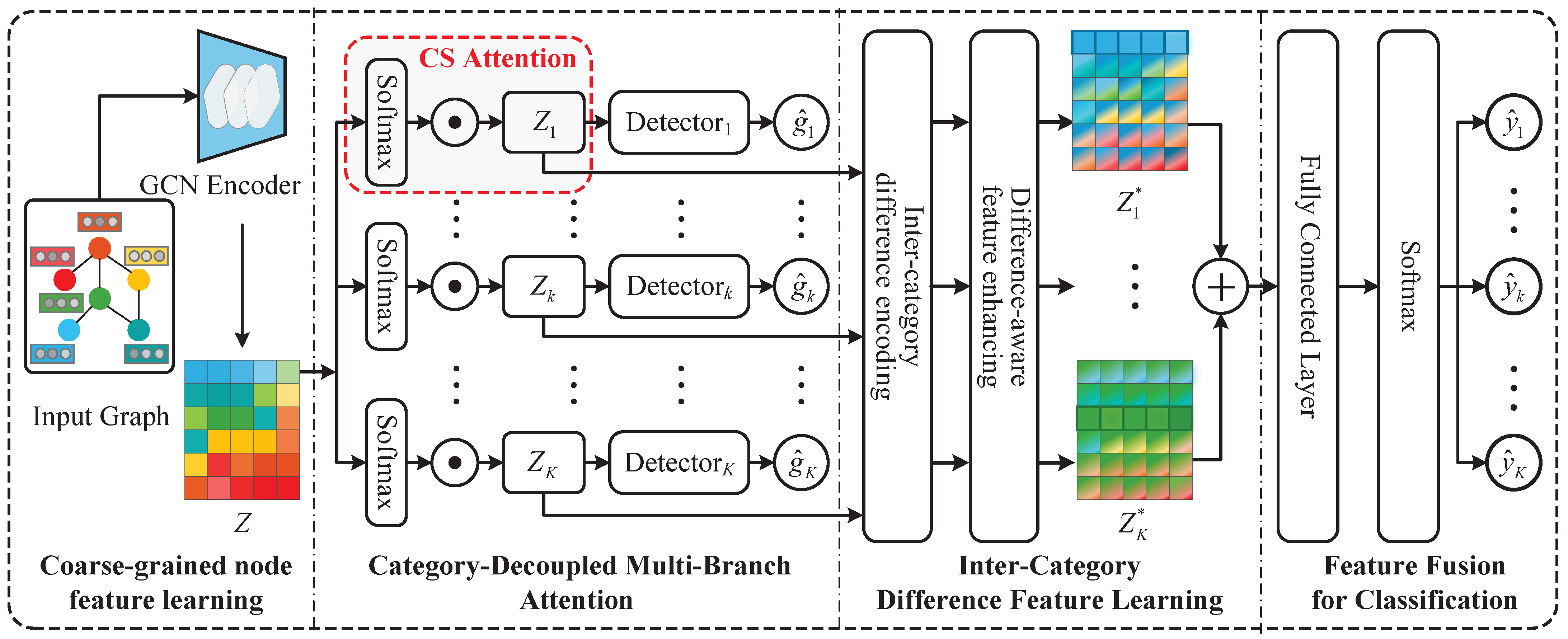
In this section, we present CA-NodeNet, a novel framework designed for node classification tasks. The overall architecture of CA-NodeNet is illustrated in
Figure 1. The proposed framework consists of three principal components: (1) a coarse-grained node feature learning module, (2) a category-decoupled multi-branch attention module, and (3) an inter-category difference feature learning module. The mathematical notations referenced throughout
Section 3 are summarized in
Table 1 for ease of reference.
3.1. Coarse-Grained Node Feature Learning Module
For simplicity and effectiveness, we employ the widely adopted GCN proposed in [
6] as the fundamental graph encoder within our framework. As illustrated in
Figure 1, the model utilizes a GCN-based encoder to generate coarse-grained node feature, defined as
, with
N being the number of nodes and
F the dimension of input node features. Specifically, a GCN leverages spectral graph theory to perform convolutional operations by propagating information between nodes and their respective neighbors. Given a graph
, where
V is the set of nodes and
E is the set of edges, the core operation of GCN involves aggregating and updating node features based on a symmetrically normalized adjacency matrix [
6]. This process enables efficient extraction of topological and feature information for effective node representation learning. For each layer, the update rule for node features is as follows:
Here, represents the node feature matrix at layer l; is the symmetrically normalized adjacency matrix; , where I is the identity matrix; is the degree matrix with self-loops. represents the weight matrix of the network at layer l, with F being the dimension of input node features and the dimension of output features. denotes . This process propagates the information of a node to its neighbors and achieves feature aggregation among nodes. Eventually, after multiple layers of GCNs, the output node’s representation can effectively capture the structural information and node features of the graph. In this paper, we employ a two-layer GCN encoder to obtain the coarse-grained node representation .
3.2. Category-Decoupled Multi-Branch Attention Module
As described in
Section 3.1, feature aggregation for each node is accomplished using a GCN-based encoder, which integrates information from a node and its neighbors according to the underlying graph topology. Building upon this encoder, we propose a category-decoupled multi-branch attention module to extract salient and category-specific discriminative features. The architecture and operation of this module are depicted in
Figure 1. The module is designed to enhance node representations by emphasizing informative features relevant to each category, thereby improving the discriminative capacity of the model.
The coarse-grained node representations, Z, are generated by utilizing a GCN-based encoder that processes the node feature matrix from the training set. With a coarse-grained node representation Z, our category-decoupled multi-branch attention module aims to learn salient and specific discriminative feature sets , where K is the number of categories. Inside the category-decoupled multi-branch attention module, we design K sub-branches for Z, in which the kth branch learns one category-specific feature for Z with respect to the kth category. Each sub-branch is composed of a category-specific attention (CS Attention) unit, a category-specific detector, and detection loss. CS Attention focuses on extracting the weights for Z with respect to category, the category-specific detector aligning with , and intermediate supervision loss, which constrains each category-specific feature over all sub-branches and is averaged from K detection losses.
Category-Specific Attention: In the context of the attention mechanism, the softmax function [
30] ensures that the computed weights are normalized to sum to one. This normalization not only facilitates focusing on task-relevant dimensions with higher attention values but also suppresses the influence of less important feature dimensions [
30], thereby enhancing the model’s discriminative capacity. We employ an attention mechanism to extract category-specific features, enhancing classification accuracy while reducing irrelevant information. Firstly, the input features are processed by a fully connected layer. Then, attention weights are computed via a softmax function and used to perform a weighted sum over the input features, forming category-specific features. Finally, these features are passed through fully connected layers and a sigmoid function for classification, enabling more precise detection. In our work, the attention mechanism provides flexibility in our model to learn
K category-specific features
from the feature
Z. As shown in
Figure 1,
K CS Attention units are used. The details of each CS Attention unit are depicted in
Figure 2. Specifically, the feature
Z is separately connected to
K fully connected layers. After activation by softmax, the attention weight of
Z is obtained for each specific category:
where
is a matrix that has the same dimensions as
Z,
is the dimension of
Z, and
. Then, the representation
for each specific category is given by the following:
where ⊙ denotes element-wise multiplication.
Category-Specific Detector: Each category-specific detector comprises two fully connected layers followed by a sigmoid layer as the output. The fully connected layers serve as classifiers, while the sigmoid layer functions as the activation mechanism, enabling the mapping of outputs to probabilities. Note that the sigmoid layer is not the only option for the detector. The
kth category-specific detector is shown in
Figure 2. For the training samples, the sub-branch for the
kth category is trained by optimizing the following detection loss:
where
and
denote the ground truth (either 1 or 0) and the probability of samples belonging to the
kth category, respectively. For example, if the category of samples is the
kth category, then the ground truth of samples in the
kth detector is 1 and that of the other detectors is 0.
allows the network to generate category-specific features for every sample.
Intermediate Supervision Loss: The category-decoupled multi-branch attention module is regulated by intermediate supervision loss, which is computed as the mean of
K detection losses derived from the sub-branches. Specifically, for each sub-branch, a distinct detection loss is calculated, and the intermediate supervision loss is defined as the average of these
K individual detection losses:
By restraining the intermediate supervision loss of and the attention mechanism, the category-decoupled multi-branch attention module obtains salient and discriminative category-aware features for node classification.
3.3. Inter-Category Difference Feature Learning Module
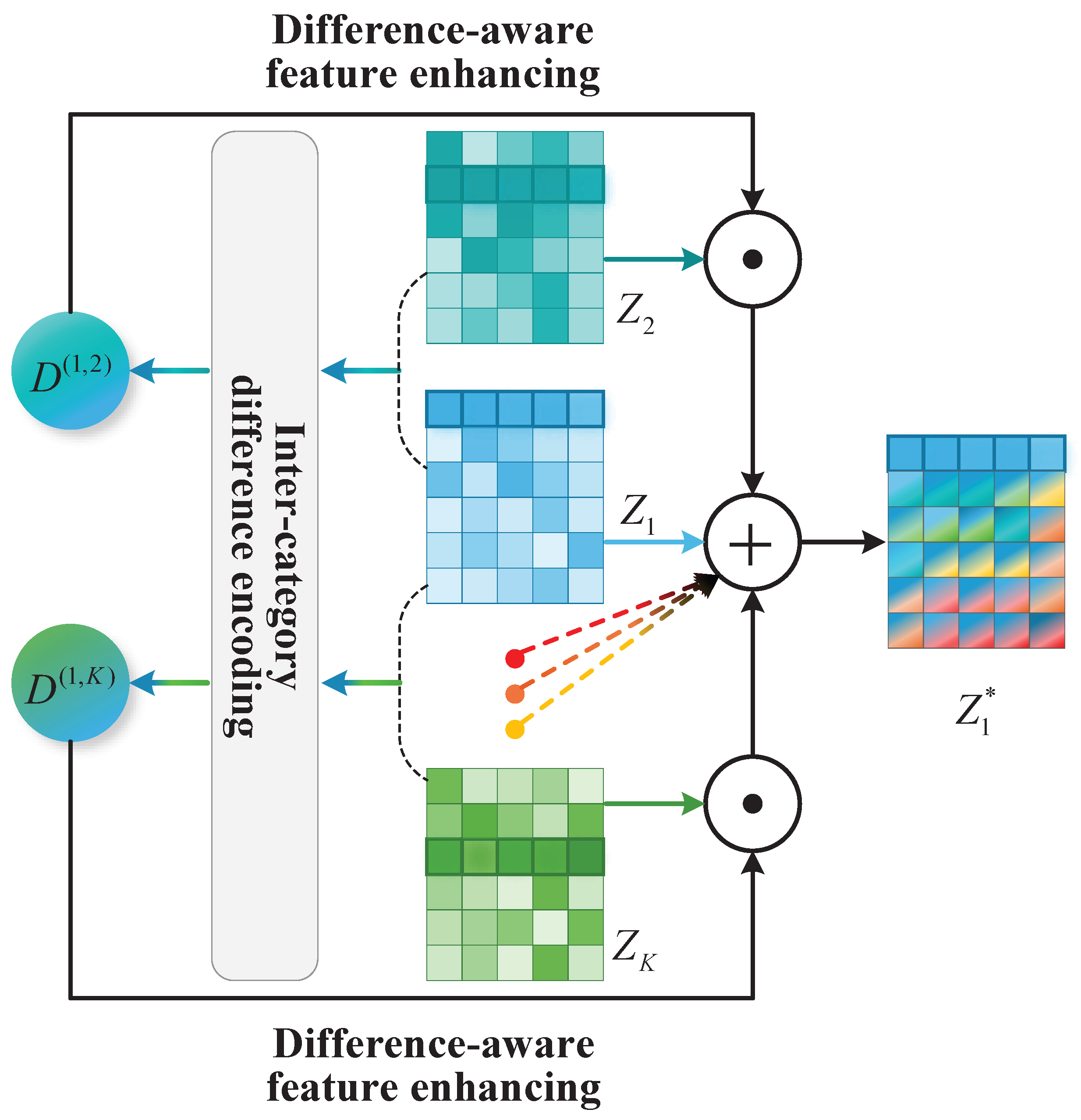
The inter-category difference feature learning module is illustrated in
Figure 3. The module computes feature differences to enhance category-specific features and strengthen the model’s capability to distinguish between different categories. This module comprises two sub-components: inter-category difference encoding and difference-aware feature enhancement. The inter-category difference encoding sub-module is responsible for quantifying pairwise differences between previously category-specific features, while the difference-aware feature enhancement sub-module further refines node representations.
Inter-Category Difference Encoding: To capture feature differences across categories, we first quantify pairwise differences between previously obtained category-specific features
. These quantified difference values are then encoded to capture the discriminative information divergence across different categories. Specifically, this scheme calculates the distances between pairwise features using the Euclidean distance and encodes these distances as metrics to quantitatively assess inter-category differences. Then, we focus on pairs of features with significant differences to extract their complementary information and use it to enhance the feature representations of the target category:
where
represents the distance between the
vth and
wth categories.
and
are the category-specific features, and tr(·) represents the trace of matrix. To precisely distinguish the differences between pairwise features, the most significant inconsistencies within each pairwise feature set are utilized to constrain the receptive field during feature enhancement, ensuring a more targeted and effective improvement of feature representations. Thus, the process of difference encoding can be defined as follows:
where
represents the difference coefficient between the
vth and
wth categories.
extracts the diagonal elements of the matrix as a vector, and
is a learnable difference weight matrix.
is a difference encoder that retains the top-
k largest distances in
and sets the rest to zero.
Difference-Aware Feature Enhancing: To ensure that each category-specific feature captures comprehensive and discriminative information, a difference-aware feature enhancement mechanism is employed. This mechanism is designed to learn and integrate complementary information from multiple pairs of feature representations. Specifically, the process of category-specific feature enhancing can be formally expressed as follows:
where
is the
vth updated feature after considering inter-category differences. By leveraging the differences across multiple categories, we effectively compensate for the complementary information within inter-category features, enhancing their representational capacity.
3.4. Feature Fusion for Classification
Following the inter-category difference feature learning module, the fusion of
K enhanced feature representations remains a significant challenge. To address this, we adopt element-wise summation to integrate all enhanced features, ensuring an efficient and unified representation. Consequently, the fuse feature representation
is defined as follows:
where
is the updated enhanced feature after considering inter-category differences.
Then, the fused feature
is fed into the final classification module, which consists of two fully connected layers. The first fully connected layer is followed by a dropout layer (with a dropout probability of 0.5). Lastly, the output of the last fully connected layer is activated by a softmax unit. Here, the cross-entropy loss for node classification over all training nodes in
X is represented as
:
where
is the set of node indices that have labels,
is the associated ground truth label vector (same as the one-hot vector),
denotes the associated prediction probabilities for the every sample,
, and
K is the number of categories.
A Dual-Component Optimization Function: The intermediate supervision loss
in Equation (5) and classification loss of
in Equation (10) are combined to construct a novel loss for all training samples:
where the hyperparameter
balances the contributions of intermediate supervision and category classification.
Finally, the model’s parameters are optimized with respect to the objective function using stochastic gradient descent. To ensure general applicability, the detailed algorithm of the proposed model is outlined in Algorithm 1.
| Algorithm 1 CA-NodeNet |
- Require:
Graph , Feature Matrix , Adjacency Matrix . - Ensure:
Node classification predictions . - 1:
Initialize model parameters . - 2:
Encode node features using a GCN-based encoder through Equation (1) to obtain Z. - 3:
for each category do - 4:
Compute CS attention weights via Equation (2) - 5:
Compute category-specific feature through Equation (3) - 6:
Train category-specific detectors using Equation (4) - 7:
end for - 8:
Calculated intermediate supervision loss via Equation (5) - 9:
for each pair of categories do - 10:
Compute difference using Equations (6) and (7) - 11:
Encode difference with top-k largest values. - 12:
Enhance features with complementary information via Equation (8) - 13:
end for - 14:
Fuse all enhanced features via Equation (9) to obtain - 15:
Feed into a classifier and compute cross-entropy loss with Equation (10) - 16:
Evaluate the loss with Equation (11) - 17:
Update the parameter set via back propagation - 18:
Return predictions .
|


