Abstract
The rapid development of wireless communication technology is leading to increasingly scarce spectrum resources, making efficient utilization a critical challenge. This paper proposes a Convolutional Neural Network–Long Short-Term Memory-Integrated Gradient-Weighted Class Activation Mapping (GC-CNN-LSTM) model, aimed at enhancing the accuracy of long-term spectrum prediction across multiple frequency bands and improving model interpretability. First, we achieve multi-frequency long-term spectrum prediction using a CNN-LSTM and compare its performance against models including LSTM, GRU, CNN, Transformer, and CNN-LSTM-Attention. Next, we use an improved Grad-CAM method to explain the model and obtain global heatmaps in the time–frequency domain. Finally, based on these interpretable results, we optimize the input data by selecting high-importance frequency points and removing low-importance time segments, thereby enhancing prediction accuracy. The simulation results show that the Grad-CAM-based approach achieves good interpretability, reducing RMSE and MAPE by 6.22% and 4.25%, respectively, compared to CNN-LSTM, while a similar optimization using SHapley Additive exPlanations (SHAP) achieves reductions of 0.86% and 3.55%.
1. Introduction
The rapid development of wireless communication technology has driven a significant increase in demand for spectrum resources, highlighting the issues of spectrum scarcity and low utilization [1]. Cognitive Radio (CR) technology is an effective solution to address this problem, allowing secondary users (SUs) to opportunistically access the licensed bands of primary users (PUs) when they are not being used [2]. Accurate detection of PU signals is crucial for SUs to efficiently utilize the spectrum [3]. However, frequent signal detection incurs additional system overhead. Given constrained sensing resources, spectrum prediction emerges as a key method for reducing channel detection costs. By analyzing historical spectrum data, this approach enables long-term joint prediction of spectral states across multiple frequency bands, allowing for rapid identification of spectrum holes. These predictions subsequently guide spectrum-sensing and decision-making processes, thereby minimizing spectrum handovers and improving utilization efficiency [4].
Spectrum prediction represents a classic time series forecasting problem, with methodological evolution progressing from traditional statistical models to contemporary deep learning techniques. Early research primarily employed regression models: Hidden Markov Models (HMM), Support Vector Machines (SVMs), Random Forest (RF), and Kalman Filter (KF) [5]. Although computationally efficient, these approaches have demonstrated limited capability in capturing complex spatiotemporal correlations when processing multi-frequency point data [1]. The emergence of neural networks has led to substantial progress, particularly in the area of spectrum prediction. Long Short-Term Memory (LSTM) networks have proven to be highly effective for this task, thanks to their excellent capabilities in modeling temporal dependencies. LSTM-based approaches substantially improve short-term prediction accuracy for individual frequency points [6]. However, conventional LSTM architectures face inherent limitations in integrating spatial dimension information, whereas multi-frequency prediction requires simultaneous capture of spatial (frequency) correlations among frequency points. Convolutional Neural Networks (CNNs) are neural networks specifically developed for two-dimensional image data. They can effectively extract spatial information from data and can also be applied to one-dimensional data, such as text sequences and time series predictions [7]. Reference [8] proposed a CNN-LSTM neural network combining CNN with LSTM that can effectively extract spatial and temporal features of residential energy consumption prediction. CNN-LSTM can adeptly discern and predict jamming behaviors, which can enhance the anti-jamming performance of communication systems [9]. Reference [10] combined CNN and LSTM to enhance the accuracy of spectrum prediction in multi-channel spectrum sharing. CNN is used for feature extraction of spectrum data, while LSTM is responsible for predicting spectrum occupancy status. Reference [11] combined seasonal decomposition (SD), ensemble empirical mode decomposition (EEMD), and CNN-LSTM to predict the temperature, wind speed, relative humidity, and precipitation in three regions of Rio de Janeiro State, Brazil. This approach significantly improved the accuracy of weather variable predictions. Reference [12] proposed a parallel CNN-LSTM-Attention model. The model makes predictions through CNN-LSTM and uses the attention mechanism to focus on learning important features, thereby improving the efficiency and accuracy of predictions. Reference [13] proposed a spectrum-sensing method based on CNN-LSTM and combined with the attention mechanism. The CNN is used to extract the relevant features in the covariance matrix, the LSTM is used to extract the temporal features from the samples, and the attention mechanism is used to enhance the focus on the channel state features, effectively improving the accuracy of spectrum sensing, especially performing well in low signal-to-noise ratio environments.
The data of spectrum prediction across different time periods and frequencies can be regarded as different characteristics when viewed in the multi-dimensional time–frequency space. Datasets with a large number of features usually contain irrelevant features, which may include unnecessary features that have a negative impact on the model’s performance. Feature selection effectively enhances the model’s accuracy, improves computational efficiency, and tends to make the model more interpretable [14]. Time series data possess chronological order and numerous interacting variables. Explaining prediction models through eXplainable Artificial Intelligence (XAI) will help identify which periods and variables in the dataset have the greatest influence, thereby assisting in feature selection. Beyond interpretability, XAI-derived explanations are increasingly applied to refine model architectures and improve training efficiency in time series prediction tasks such as spectrum forecasting. This reflects a growing trend where explanations are not merely tools for understanding model behavior but are actively used to enhance prediction accuracy and model optimization [15,16]. Reference [17] provides a detailed account of the current application status of XAI in time series prediction, offering a comprehensive overview and guidance for research. Reference [18] employed LSTM to predict energy consumption. They introduced XAI methods to provide a more transparent underlying mechanism and decision-making process, identified the parameters that significantly influence the model output, and supported energy allocation decisions. Gradient-weighted class activation mapping (Grad-CAM) was originally designed to explain the output of the image spectrum repository [19]. It uses gradients to analyze how the features from the final convolution layer affect the classification. It has now been applied to time series prediction [20]. Research has employed multi-head CNN for time series energy prediction and utilized Grad-CAM and SHAP for interpretation. Both XAI methods are able to enhance prediction accuracy and model efficiency by identifying and eliminating irrelevant features. Reference [21] employed occlusion sensitivity, Local Interpretable Model-Agnostic Explanations (LIMEs), and Grad-CAM to interpret a power quality disturbance classifier. The results demonstrate that the combination of CNN and Grad-CAM achieves good predictive performance and interpretability. Similarly, a recent study on laser powder bed fusion (LPBF) [22] employed frequency analysis and Grad-CAM to track the movement and location of the acoustic emission source. This indicates that XAI can clarify the relationship between process parameters and acoustic signals, thereby enhancing the real-time monitoring capability. Another study [23] combined machine learning (ML) and XAI for real-time cavity profile prediction in electrochemical machining (ECM). The research proved that XAI can make ML models more accurate and more physically understandable, which is crucial for optimizing parameters and identifying problems in complex processes. These examples demonstrate that XAI is very powerful in many complex engineering fields, helping to improve performance and quality assurance.
After investigation, research on the interpretability of the CNN-LSTM composite network time series prediction model has not been reported yet. Therefore, a GC-CNN-LSTM model based on improved Grad-CAM is proposed to enhance model interpretability and improve prediction accuracy. The main contributions of this study are as follows:
- Multi-frequency long-term spectrum prediction was achieved using CNN-LSTM, and it was compared with LSTM, GRU, CNN, Transformer, and CNN-LSTM-Attention. The advantages and disadvantages of the current prediction method were tested.
- The GC-CNN-LSTM method was used to conduct a time–frequency global interpretation of the model, where model inputs were selectively based on the feature importance obtained through Grad-CAM’s interpretation in both the time and frequency domains.
- The performance of the proposed scheme was evaluated through extensive simulations. The simulation results show that the GC-CNN-LSTM algorithm can effectively improve the accuracy of spectrum prediction and provide superior interpretability compared to SHAP.
2. Problem Modeling
The objective of multi-frequency long-term spectrum prediction is to forecast the future spectrum occupancy status based on historical data, with the input data being the historical time–frequency data matrix:
where represents the input matrix of the model, represents the input step size, and represents the input spectral width.
The time–frequency data prediction output for the future frequency band is
where represents the output matrix of the model, represents the prediction step size, and represents the prediction spectral width.
The spectrum data perceived through sensing are uniformly distributed in the frequency domain. Selecting the appropriate spectrum data for prediction is a key issue. Traditional feature selection methods rely on calculating the correlations between features and the prediction targets, such as computing the Pearson correlation coefficients using principal component analysis [24]. However, these methods have limited effectiveness and are not suitable for multi-frequency prediction. Meanwhile, neural network models are typically black-box models, which introduce uncertainties and reduce the credibility of prediction results. Since the input data were generated sequentially using time windows, the feature importance values calculated by SHAP were mainly based on the information within individual windows and may not fully reflect the overall temporal feature importance in the entire dataset. To address the interpretability challenges in time–frequency prediction models, we have improved the Grad-CAM method to enable global interpretation of multi-frequency long-term prediction models.
3. Model Construction
3.1. CNN-LSTM
CNN-LSTM is a powerful hybrid neural network architecture that combines CNN and LSTM networks to handle spatial and temporal features in data. The CNN-LSTM model primarily consists of a signal input layer, convolutional layers, pooling layers, LSTM layers, and fully connected layers. CNN-LSTM can extract the complex features from time–frequency spectral data through the convolutional layers in the CNN and is good at capturing complex spatiotemporal patterns in datasets with nonlinear characteristics, making it highly suitable for applications involving the analysis of spatiotemporal data [25]. Figure 1 shows the model architecture.
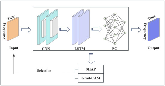
Figure 1.
Model framework diagram.
The multi-frequency long-term prediction process based on CNN-LSTM is as follows. Firstly, the input time–frequency signal matrix is normalized and input into the CNN convolutional layer, where features are adaptively extracted using convolution kernels as
The equation denotes the convolution operation of the filter on the input, where represents the input time–frequency matrix, represents the filter, represents the bias, and ReLU (Rectified Linear Unit) represents the linear rectification function, which is a non-linear activation function:
Then, we perform pooling operations through the max-pooling layer on the extracted features to reduce data dimensionality while retaining the main feature information.
where MaxPool represents maximum pooling, which is used to extract the maximum feature data within a specified window.
Using the data after dimensionality reduction with the CNN as the feature input for the LSTM layer, the neural network is trained to automatically learn sequence features. The training error is back-propagated using the Adam algorithm, and the model parameters are updated layer by layer. Finally, the ReLU activation function is used to classify the signal features, completing the multi-frequency long-term prediction task.
The core of LSTM is the memory cell, which includes three gating mechanisms.
The forget gate decides which information to discard from the memory unit:
The input gate determines which new information is stored in the memory unit:
The state of the candidate memory unit is
The output gate determines which information is output from the memory unit:
The state of the memory unit is updated as
The hidden state is
In the above formula, represents the input at the current time step, represents the hidden state of the previous time step, represents the memory unit state of the previous time step, and represent the learnable weights and biases, represents the Sigmoid activation function, and represents the hyperbolic tangent activation function.
3.2. Improved Grad-CAM
Grad-CAM leverages the gradient signals flowing into the final convolutional layer of a CNN to judge the contribution of each neuron toward a target decision [19]. It is widely applied in tasks such as image classification [19], image captioning [26], and visual question answering [27]. In contrast to the conventional Grad-CAM framework, designed for classification, our study addresses a regression problem. Furthermore, the objective function is formulated as the mean value because the predicted quantity is a time–frequency data matrix rather than a scalar.
The objective function, , is the average value of all elements in the prediction output matrix, , where the dimension of is . Specifically, represents the size of the time dimension, and represents the size of the frequency dimension. The formula calculates the sum of all elements in the matrix through a double loop for summation. Finally, the sum is divided by the total number of elements in the matrix to obtain the objective value.
Grad-CAM selects the last convolutional layer of the CNN as the target and calculates the gradient of the objective function with respect to the output of the convolutional layer as
where represents the output feature matrix of the second convolutional layer, represents the number of time steps after multiple pooling operations, and represents the number of channels of the convolutional layer.
Next, we calculate the gradient of the objective function with respect to the output A2 of the convolutional layer as
where [1, is the time step index, and [1, is the channel index.
For each channel , its average gradient across the time dimension is calculated as the importance weight of that channel:
The feature maps, , of each channel are summed according to the weights, ; then, the ReLU activation function is applied to obtain the class activation map:
The Grad-CAM results are up-sampled back to the original temporal resolution as
The above steps calculate the importance of a single input of the model for the output using the Grad-CAM method. The original Grad-CAM provides local explanations for single predictions. In the context of our time series prediction model, which uses a fixed-length window of data for each prediction step, the original Grad-CAM can only explain the activations related to that single step. In contrast, our improved Grad-CAM method is designed to provide global explanations for the entire dataset. To obtain the global class activation mapping image, this method needs to be improved. The method we adopted performs cyclically stacking and averaging. The total duration of the training data is , and the training set, , is generated through the window sliding method. Each training session produces a prediction result, and at the same time, a class activation mapping image is generated:
where is the class activation map generated by the th training sample.
For the initial time point, a single class activation mapping image is incorporated. At the subsequent time point, two such images are included. This pattern progresses such that, from the -th time point onward, class activation mapping images are encompassed. By averaging the values of corresponding time points across these images, a global class activation mapping image is derived:
where is the average of the CAM values of all the windows covering that time point, is the set of all window indices covering time , represents the number of windows covering time point t, and represents the value at time point in the -th CAM graph.
The final global class activation map, , can be represented as
3.3. Evaluation Metrics
The evaluation metrics adopted are the Root Mean Squared Error (RMSE) and the Mean Absolute Percentage Error (MAPE) [28]. The RMSE is defined as the square root of the average of the squared differences between the predicted and actual values, making it more sensitive to larger errors. The MAPE is the average of the relative percentage differences between the predicted and actual values. The formulas for these metrics are calculated as
where represents the true value, represents the predicted value, and represents the number of samples.
3.4. Simulation Setup
The simulation dataset was obtained from the Electrosense open spectrum repository [29], encompassing a frequency range of 1300–1764 MHz with a 2 MHz resolution. This dataset comprises 2661 time series samples, each collected at 1 min intervals, with their time–frequency attributes depicted in Figure 2. The spectral data was gathered by outdoor sensors stationed in Madrid, Spain. The sensors were configured to capture data within the 1300–1764 MHz frequency range, with a frequency resolution of 2000 kHz (or 2 MHz) and a time interval of 1 min. The dataset consists of 2661 time slots across 232 frequency points, each representing the signal-to-noise ratio (SNR) of the signal in decibels (dB).
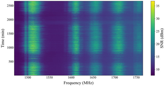
Figure 2.
Time–frequency spectrum heatmap.
As shown in Figure 2, the spectral data is organized in a band pattern with distinct intervals. Areas colored in blue indicate a lower SNR, which is favorable for communication purposes within this frequency band due to less interference. In contrast, the red areas denote a higher SNR, implying that these frequency bands are potentially more congested with signals.
The computer configuration includes an Intel Core i7-13650 CPU, 16 GB of memory, and an RTX 4060 GPU. The comparative models include LSTM [30], GRU [31], CNN [7], Transformer [32], CNN-LSTM [10], and CNN-LSTM-Attention [33]. The hyperparameters for all models are listed in the Appendix A. The input time steps are set to 24, with the full frequency range used as the input. There are 12 prediction time steps, and the prediction frequency bandwidth is 15 (covering 15 frequency points). The training and testing datasets are split in an 8:2 ratio. The training period is 70 epochs, with each epoch consisting of 50 iterations, and the results are averaged over these iterations.
4. Simulation Results and Analysis
4.1. CNN-LSTM Model Prediction Results
The simulation results of prediction based on the measured spectrum data are shown in the following figure, where Figure 3 and Figure 4 compare the models in the temporal dimension, and Figure 5 and Figure 6 compare them in the frequency dimension. As can be seen from the figures, the prediction performance of CNN-LSTM is superior to that of LSTM, GRU, and CNN. The Transformer model has a performance close to CNN-LSTM in terms of MAPE, with values of 8.49% and 8.46%, respectively. However, the RMSE of CNN-LSTM is lower than that of the Transformer model, indicating that the prediction errors of CNN-LSTM are more evenly distributed. The CNN-LSTM-Attention model shows slightly better prediction performance than CNN-LSTM. However, since the frequency has not been filtered, the model is more complex. Although the attention mechanism does improve the performance to some extent, the improvement is not significant. Reference [34] attributed attention’s efficacy to introducing high-order non-linearity for regularization. In our case, the powerful CNN-LSTM model already captures the necessary complexities, and the LSTM’s non-linear dynamics inherently fulfill this role, leaving little room for improvement from an additional attention mechanism.
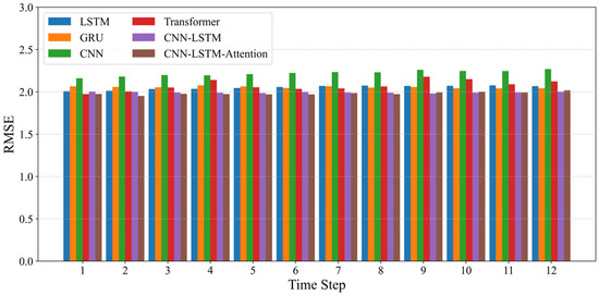
Figure 3.
Prediction performance in the temporal dimension (RMSE).
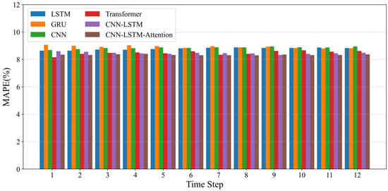
Figure 4.
Prediction performance in the temporal dimension (MAPE).
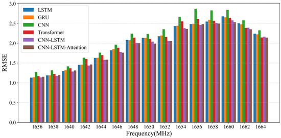
Figure 5.
Prediction performance in the frequency dimension (RMSE).
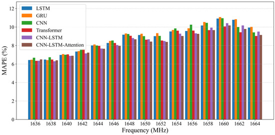
Figure 6.
Prediction performance in the frequency dimension (MAPE).
Table 1 shows the average of the results for all time–frequency points in the prediction matrix. It can be seen that the CNN has a higher RMSE than the comparative models, which indicates that it is more sensitive to larger errors. Although CNN-LSTM and CNN-LSTM-Attention show a significant decrease in MAPE, there is no significant improvement in RMSE.

Table 1.
Comparison of results from different prediction models.
4.2. Explainability Analysis
4.2.1. SHAP Explanation Results
First, we conducted an interpretable analysis of the CNN-LSTM model using SHAP. SHAP is a versatile model interpretability method that constructs an additive explanation model to calculate the contribution of all input frequencies to the prediction results. In the simulation, we utilized the GradientExplainer as the SHAP explainer. Specifically, we employed the entire training dataset as the background dataset to ensure that the model’s explanations are widely representative. Additionally, we calculated the SHAP values using the entire testing dataset to ensure accuracy and reliability.
Figure 7 shows the top 30 frequencies in terms of prediction importance for the CNN-LSTM model. Since the input data were generated sequentially using time windows, the SHAP analysis was performed locally within each window and did not incorporate global temporal dynamics across windows.
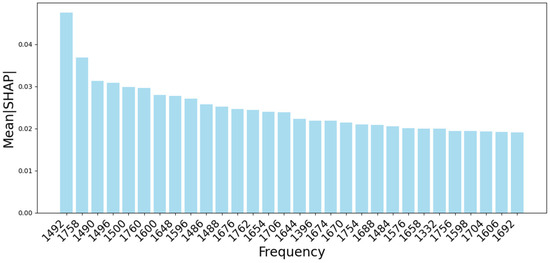
Figure 7.
SHAP interpretation results.
Table 2 shows the results of optimizing model inputs by selecting certain frequencies using SHAP. It can be seen that SHAP has improved the prediction performance of the model. The overall performance is best when retaining 75 frequency values. In this case, the RMSE and MAPE are, respectively, reduced by 0.86% and 3.55% compared to CNN-LSTM. Although the model’s MAPE is improved after frequency selection by SHAP, the improvement in RMSE is not obvious, and there are even negative effects in certain cases. The results indicate that SHAP has limited interpretability for this complex multi-frequency long-term prediction and cannot effectively reduce model fluctuations.

Table 2.
Model performance comparison under the guidance of SHAP values, retaining different numbers of frequencies. (The symbol “↓” represents a decrease.)
4.2.2. GC-CNN-LSTM Explanation Results
Figure 8, generated by the improved Grad-CAM method, serves as a visual representation of the significance of various data points for the CNN-LSTM model’s prediction. The heatmap’s horizontal axis denotes time in minutes, and the vertical axis represents frequency in MHz. The color intensity, with red indicating higher influence and blue indicating lower influence, allows for the identification of key frequency and time areas that significantly impact predictions.
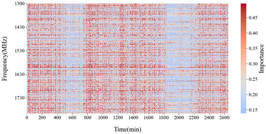
Figure 8.
Global heatmap.
By focusing on these aspects, the interpretability and transparency of the model have been enhanced. Specifically, the improved Grad-CAM calculates a global heatmap, directly visualizing which specific time–frequency regions are most influential on the model’s predictions. This visual tool is crucial for model optimization, enabling targeted adjustments to the model’s input data. The presence of periodic red areas suggests that certain frequencies have a regular impact on predictions, which could inform the refinement of the model’s temporal window settings. In summary, the heatmap enables the selection of the optimal time intervals and frequency bands for spectrum sensing, thereby enhancing the efficiency and prediction performance of the model.
Figure 9 and Figure 10 show the simulation results of the GC-CNN-LSTM model. On the one hand, frequencies with higher importance were selected as inputs from the frequency domain perspective, and the simulation retained 15, 30, 45, 60, 75, 90, 105, and 120 frequency points. On the other hand, the entire time period was divided into 48 segments, and their importance was ranked using improved Grad-CAM. Some unimportant time segments were then removed. The simulation removed 0, 1, 2, 3, 4, 5, 6, 7, 8, 9, and 10 segments. Removing zero segments means that no adjustments were made to the input data in the temporal dimension. As can be seen from the figures, its prediction performance is worse than that of the other cases where some time segments were removed, especially in terms of RMSE. This result demonstrates the effectiveness of the approach of removing some time segments.
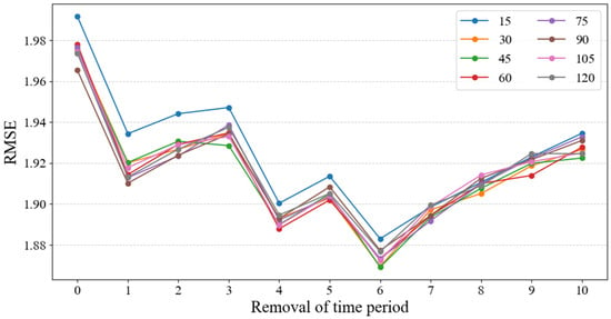
Figure 9.
Simulation results of GC-CNN-LSTM model prediction (RMSE).
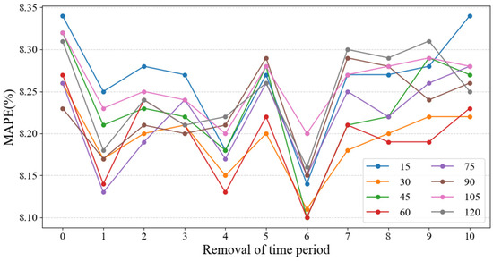
Figure 10.
Simulation results of GC-CNN-LSTM model prediction (MAPE).
By carefully selecting frequencies and removing some time segments, the model performance can be significantly improved. Overall, the optimal prediction performance was achieved by retaining forty-five input frequencies while removing the six least important time segments. Under these circumstances, the RMSE was 1.8692, and the MAPE was 8.1%, achieving improvements of 6.22% and 4.25% compared with the baseline CNN-LSTM model, respectively. The results show that the approach provides better model interpretation and optimization than SHAP, especially in terms of reducing the RMSE significantly and minimizing prediction anomalies.
The completed simulations were based on the 1650 MHz frequency band. To verify the robustness of the model, we also conducted predictions for two other frequency bands (1550 MHz and 1750 MHz), as shown in Table 3.

Table 3.
Model performance across frequency bands. (The symbol “↓” represents a decrease.)
In the scenario where forty-five input frequencies are retained and the six least significant time segments are excluded, a detailed statistical comparison was conducted between the GC-CNN-LSTM and CNN-LSTM models using Welch’s unequal variances t-test [35]. The analysis, as presented in Table 4, reveals the GC-CNN-LSTM model’s superior predictive performance. The RMSE results for the GC-CNN-LSTM model show a notable decrease, with a t-statistic of 6.247 and a p-value less than 0.001. Correspondingly, the MAPE also indicates a substantial reduction, with a t-statistic of 3.760 and a p-value of 0.00018.

Table 4.
t-test analysis of CNN-LSTM and GC-CNN-LSTM.
Figure 11 offers a graphical comparison of the RMSE and MAPE between the two models. The GC-CNN-LSTM model displays a lower median error and a tighter spread in both metrics, implying more reliable and accurate forecasting. The 95% confidence intervals for RMSE ([4.26%, 8.18%]) and MAPE ([2.03%, 6.48%]) reinforce the statistical significance of these improvements. These findings collectively demonstrate that the GC-CNN-LSTM model significantly enhances predictive accuracy in comparison to the CNN-LSTM model.
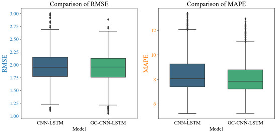
Figure 11.
Box plots of RMSE and MAPE for CNN-LSTM vs. GC-CNN-LSTM.
4.3. Efficiency Analysis
In addition to predictive performance, the efficiency of models in terms of computational time is crucial for practical applications. This section presents an analysis of the time consumption for each model listed in our study. To ensure a fair comparison, all models were trained for 70 epochs. From Table 5, we can see that the training time for the SHAP-CNN-LSTM and GC-CNN-LSTM models is shorter than that of CNN-LSTM because they filter the input features in the frequency domain. Particularly, the GC-CNN-LSTM model filters inputs both in the time and frequency domains, which not only enhances the predictive accuracy but also decreases the time consumption for predictions.

Table 5.
Time consumption of different models.
4.4. Discussion
Using the improved Grad-CAM method, the time periods and frequency bands were successfully identified and sorted. This enhancement allows for more efficient allocation of sensing resources, as the system can now focus on the most critical time–frequency regions. Specifically, the improved GC-CNN-LSTM model has higher interpretability and prediction accuracy, which enables the spectral sensing decision to be more precise and timelier. For instance, in the context of Dynamic Spectrum Access (DSA) and CR networks, this means that secondary users can more effectively identify and utilize the unused spectrum bands, thereby improving overall spectral efficiency [1,6].
The demonstrated reductions in RMSE by 6.22% and MAPE by 4.25% relative to the baseline CNN-LSTM model, along with superior performance compared to SHAP-based optimization, substantiate the efficacy of XAI not only as a tool for model interpretation but also as a robust methodology for active feature selection and input optimization. These findings resonate with applications in energy forecasting [18,20] and financial time series [7], where XAI has improved both transparency and predictive outcomes.
A key limitation of the proposed model is its reliance on purely data-driven learning, which may compromise its generalizability to environments featuring unseen propagation conditions or user dynamics. This limitation aligns with challenges documented in domains such as power quality analysis [24] and medical forecasting [32]. This highlights a common problem in applied AI, in that data-based models often do not match the behavior of real-world physical systems. Future research could focus on developing hybrid models that combine data-driven approaches with the physical principles of signal propagation. This integration could enhance the robustness and reliability of AI models in spectrum prediction, particularly in environments with varying signal characteristics.
From a practical standpoint, this study enhances CR efficiency by reducing sensing costs and unnecessary interference. Moreover, the proposed feature selection strategy, guided by Grad-CAM, holds substantial promise for other domains involving multi-dimensional time series data, including energy demand forecasting [8,20], algorithmic trading [7], and industrial Internet of Things (IoT) [24]. The transparency afforded by Grad-CAM also helps overcome trust-related barriers to AI adoption in critical applications, facilitating clearer operational insights for engineers and stakeholders [14,17].
To address data limitations, future work could explore data augmentation strategies such as virtual sample generation (VSG). As shown in [36], VSG can effectively enlarge training sets and improve prediction accuracy for ML-based data-driven models in engineering domains with limited experimental data. This approach could be adapted to spectrum prediction to mitigate data scarcity issues and enhance model performance and generalizability.
5. Conclusions
This paper mainly focused on the accuracy and interpretability of multi-frequency long-term spectrum prediction. We developed the GC-CNN-LSTM model, incorporating a novel Grad-CAM architecture to explain the CNN-LSTM mechanism. The improved Grad-CAM technique can generate global heatmaps that visually reveal the influence of different time segments and frequency bands on predictions, offering comprehensive explanations. Simulations with the GC-CNN-LSTM model demonstrated that selectively retaining key frequencies and pruning insignificant time segments reduced RMSE and MAPE by 6.22% and 4.25%, respectively, which was superior to that of SHAP. The results validated the effectiveness of the proposed approach in model interpretation and optimization. It provided a practical and explainable method for multi-frequency long-term spectrum prediction and facilitated spectrum sensing applications.
Author Contributions
Conceptualization, J.Z.; Formal analysis, W.X. and Z.S.; Funding acquisition, J.Z.; Investigation, W.X.; Methodology, W.X., J.Z. and Z.S.; Project administration, J.Z.; Supervision, J.Z.; Writing—original draft, W.X.; Writing—review and editing, J.Z., Z.S. and L.J. All authors have read and agreed to the published version of the manuscript.
Funding
This work was supported by the National Natural Science Foundation of China under Grant 62231012.
Data Availability Statement
The dataset was obtained from the Electrosense open spectrum repository [29]. The source code of the experiments presented in this paper is available upon request from the corresponding author.
Conflicts of Interest
The authors declare no conflicts of interest.
Appendix A. Model Architectures
Appendix A.1. LSTM, GRU, CNN, CNN-LSTM, and CNN-LSTM-Attention
The following table shows the architecture of the CNN-LSTM model. The CNN model is a simplified version of this, excluding the LSTM layers, and the LSTM model excludes the convolutional layers. The GRU model has the same structure as the LSTM model, with the only difference being the replacement of Layer Type with GRU. The CNN-LSTM-Attention model is an extension of the table provided, where an additional TimeDistributed Self-Attention (num_heads = 4, key_dim = 8) layer is added after the second LSTM layer.

Table A1.
CNN-LSTM model architecture.
Table A1.
CNN-LSTM model architecture.
| Module | Layer Type | Parameters | Activation Function |
|---|---|---|---|
| Input | Input | input_shape = (seq_len, freqs) | |
| 1st Conv Block | Conv1D | filters = 64, kernel_size = 3 | ReLU |
| MaxPooling1D | pool_size = 2 | ||
| Dropout | rate = 0.2 | ||
| 2nd Conv Block | Conv1D | filters = 32, kernel_size = 3 | ReLU |
| MaxPooling1D | pool_size = 2 | ||
| Dropout | rate = 0.2 | ||
| 1st LSTM | LSTM | units = 64, return_sequences = True | Tanh |
| Dropout | rate = 0.2 | ||
| 2st LSTM | LSTM | units = 32, return_sequences = False | Tanh |
| Dropout | rate = 0.2 | ||
| Fully Connected | Dense | units = 64 | ReLU |
| Output | Dense | output_size = pred_steps × pred_freqs | Linear |
| Compile | Optimizer | Adam(learning_rate = 0.001) | |
| Loss | MSE | ||
| Training Settings | Epochs | 70 | |
| Batch Size | 32 | ||
| Validation Split | 0.2 |
Appendix A.2. Transformer

Table A2.
Transformer model architecture.
Table A2.
Transformer model architecture.
| Module | Layer Type | Parameters | Activation Function |
|---|---|---|---|
| Input | Input | input_shape = (seq_len, freqs) | |
| Preprocessing | Positional Encoding | Custom function | |
| Dropout | rate = 0.2 | ||
| Core Block | Transformer Encoder | head_size = 128, num_heads = 4, ff_dim = 8 | ReLU |
| Sequence Pooling | GlobalAverage-Pooling1D | -- | |
| Dropout | rate = 0.2 | ||
| Fully Connected | Dense | units = 64 | |
| Output | Dense | output_size = pred_steps × pred_freqs | Linear |
| Compile | Optimizer | Adam(learning_rate = 0.001) | |
| Loss | MSE | ||
| Training Settings | Epochs | 70 | |
| Batch Size | 32 | ||
| Validation Split | 0.2 |
References
- Shawel, B.S.; Woldegebreal, D.H.; Pollin, S. Convolutional LSTM-based long-term spectrum prediction for dynamic spectrum access. In Proceedings of the 2019 27th European Signal Processing Conference (EUSIPCO), A Coruna, Spain, 2–6 September 2019; pp. 1–5. [Google Scholar]
- Haykin, S. Cognitive radio: Brain-empowered wireless communications. IEEE J. Sel. Areas Commun. 2005, 23, 201–220. [Google Scholar] [CrossRef]
- Solanki, S.; Dehalwar, V.; Choudhary, J. Deep learning for spectrum sensing in cognitive radio. Symmetry 2021, 13, 147. [Google Scholar] [CrossRef]
- Wang, L.; Hu, J.; Jiang, R.; Chen, Z. A deep long-term joint temporal–spectral network for spectrum prediction. Sensors 2024, 24, 1498. [Google Scholar] [CrossRef] [PubMed]
- Wang, L.; Hu, J.; Jiang, D.; Zhang, C.; Jiang, R.; Chen, Z. Deep Learning Models for Spectrum Prediction: A Review. IEEE Sens. J. 2024, 24, 28553–28575. [Google Scholar] [CrossRef]
- Pan, G.; Yau, D.K.Y.; Zhou, B.; Wu, Q. Deep Learning for Spectrum Prediction in Cognitive Radio Networks: State-of-the-Art, New Opportunities, and Challenges. IEEE Netw. 2025, early access. [Google Scholar] [CrossRef]
- Durairaj, D.M.; Mohan, B.H.K. A convolutional neural network based approach to financial time series prediction. Neural Comput. Appl. 2022, 34, 13319–13337. [Google Scholar] [CrossRef] [PubMed]
- Kim, T.Y.; Cho, S.B. Predicting residential energy consumption using CNN-LSTM neural networks. Energy 2019, 182, 72–81. [Google Scholar] [CrossRef]
- Jia, L.; Qi, N.; Su, Z.; Chu, F.; Fang, S.; Wong, K.-K.; Chae, C.-B. Game theory and reinforcement learning for anti-jamming defense in wireless communications: Current research, challenges, and solutions. IEEE Commun. Surv. Tutor. 2024, 27, 1798–1838. [Google Scholar] [CrossRef]
- Zhang, L.; Jia, M. Accurate spectrum prediction based on joint LSTM with CNN toward spectrum sharing. In Proceedings of the 2021 IEEE Global Communications Conference (GLOBECOM), Madrid, Spain, 7–11 December 2021; pp. 1–6. [Google Scholar]
- Coutinho, E.R.; Madeira, J.G.F.; Borges, D.G.F.; Springer, M.V.; de Oliveira, E.M.; Coutinho, A.L.G.A. Multi-step forecasting of meteorological time series using CNN-LSTM with decomposition methods. Water Resour. Manag. 2025, 39, 3173–3198. [Google Scholar] [CrossRef]
- Chung, W.H.; Gu, Y.H.; Yoo, S.J. District heater load forecasting based on machine learning and parallel CNN-LSTM attention. Energy 2022, 246, 123350. [Google Scholar] [CrossRef]
- Pan, X.; Cao, K. Spectrum sensing based on CNN-LSTM with attention for cognitive radio networks. In Proceedings of the 2023 8th International Conference on Intelligent Informatics and Biomedical Sciences (ICIIBMS), Okinawa, Japan, 23–25 November 2023; Volume 8, pp. 63–67. [Google Scholar]
- Saeys, Y.; Inza, I.; Larranaga, P. A review of feature selection techniques in bioinformatics. Bioinformatics 2007, 23, 2507–2517. [Google Scholar] [CrossRef]
- Schwalbe, G.; Finzel, B. A comprehensive taxonomy for explainable artificial intelligence: A systematic survey of surveys on methods and concepts. Data Min. Knowl. Discov. 2024, 38, 3043–3101. [Google Scholar] [CrossRef]
- Vilone, G.; Longo, L. Explainable artificial intelligence: A systematic review. arXiv 2020, arXiv:2006.00093. [Google Scholar] [CrossRef]
- Theissler, A.; Spinnato, F.; Schlegel, U.; Guidotti, R. Explainable AI for time series classification: A review, taxonomy and research directions. IEEE Access 2022, 10, 100700–100724. [Google Scholar] [CrossRef]
- Maarif, M.R.; Saleh, A.R.; Habibi, M.; Fitriyani, N.L.; Syafrudin, M. Energy usage forecasting model based on long short-term memory (LSTM) and eXplainable artificial intelligence (XAI). Information 2023, 14, 265. [Google Scholar]
- Selvaraju, R.R.; Cogswell, M.; Das, A.; Vedantam, R.; Parikh, D.; Batra, D. Grad-cam: Visual explanations from deep networks via gradient-based localization. In Proceedings of the IEEE International Conference on Computer Vision, Venice, Italy, 22–29 October 2017; pp. 618–626. [Google Scholar]
- Van Zyl, C.; Ye, X.; Naidoo, R. Harnessing eXplainable artificial intelligence for feature selection in time series energy forecasting: A comparative analysis of Grad-CAM and SHAP. Appl. Energy 2024, 353, 122079. [Google Scholar] [CrossRef]
- Machlev, R.; Perl, M.; Belikov, J.; Levy, K.Y.; Levron, Y. Measuring explainability and trustworthiness of power quality disturbances classifiers using XAI—Explainable artificial intelligence. IEEE Trans. Ind. Inform. 2021, 18, 5127–5137. [Google Scholar] [CrossRef]
- Wu, M.; Shukla, S.; Vrancken, B.; Verbeke, M.; Karsmakers, P. Data-Driven Approach to Identify Acoustic Emission Source Motion and Positioning Effects in Laser Powder Bed Fusion with Frequency Analysis. Procedia CIRP 2025, 133, 531–536. [Google Scholar] [CrossRef]
- Wu, M.; Yao, Z.; Verbeke, M.; Karsmakers, P.; Gorissen, B.; Reynaerts, D. Data-driven models with physical interpretability for real-time cavity profile prediction in electrochemical machining processes. Eng. Appl. Artif. Intell. 2025, 160, 111807. [Google Scholar] [CrossRef]
- Xie, W.; Zhu, Y.; Cao, W.; Pan, J.; Wu, B.; Liu, S.; Ji, Y. PCA-LSTM anomaly detection and prediction method based on time series power data. In Proceedings of the 2022 China Automation Congress (CAC), Xiamen, China, 25–27 November 2022; pp. 5537–5542. [Google Scholar]
- Lee, S.W.; Kim, H.Y. Stock market forecasting with super-high dimensional time-series data using ConvLSTM, trend sampling, and specialized data augmentation. Expert Syst. Appl. 2020, 161, 113704. [Google Scholar]
- Sun, J.; Lapuschkin, S.; Samek, W.; Binder, A. Understanding image captioning models beyond visualizing attention. arXiv 2020, arXiv:2001.01037. [Google Scholar]
- Sarkar, A.; Rahnemoonfar, M. Grad-Cam aware supervised attention for visual question answering for post-disaster damage assessment. In Proceedings of the 2022 IEEE International Conference on Image Processing (ICIP), Bordeaux, France, 16–19 December 2022; pp. 3783–3787. [Google Scholar]
- Zhou, Y.; He, X.; Montillet, J.P.; Wang, S.; Hu, S.; Sun, X.; Huang, J.; Ma, X. An improved ICEEMDAN-MPAGRU model for GNSS height time series prediction with weighted quality evaluation index. GPS Solut. 2025, 29, 113. [Google Scholar] [CrossRef]
- Rajendran, S.; Calvo-Palomino, R.; Fuchs, M.; van den Bergh, B.; Cordobes, H.; Giustiniano, D.; Pollin, S.; Lenders, V. Electrosense: Open and big spectrum data. IEEE Commun. Mag. 2017, 56, 210–217. [Google Scholar] [CrossRef]
- Zuo, P.L.; Wang, X.; Linghu, W.; Sun, R.; Peng, T.; Wang, W. Prediction-based spectrum access optimization in cognitive radio networks. In Proceedings of the 2018 IEEE 29th Annual International Symposium on Personal, Indoor and Mobile Radio Communications (PIMRC), Bologna, Italy, 9–12 September 2018; pp. 1–7. [Google Scholar]
- Yu, L.; Guo, Y.; Wang, Q.; Luo, C.; Li, M.; Liao, W.; Li, P. Spectrum availability prediction for cognitive radio communications: A DCG approach. IEEE Trans. Cogn. Commun. Netw. 2020, 6, 476–485. [Google Scholar] [CrossRef]
- Tang, Y.; Zhang, Y.; Li, J. A time series driven model for early sepsis prediction based on transformer module. BMC Med. Res. Methodol. 2024, 24, 23. [Google Scholar] [CrossRef]
- Cui, B.; Liu, M.; Li, S.; Jin, Z.; Zeng, Y.; Lin, X. Deep learning methods for atmospheric PM2. 5 prediction: A comparative study of transformer and CNN-LSTM-attention. Atmos. Pollut. Res. 2023, 14, 101833. [Google Scholar] [CrossRef]
- Ye, X.; He, Z.; Heng, W.; Li, Y. Toward understanding the effectiveness of attention mechanism. AIP Adv. 2023, 13, 035019. [Google Scholar] [CrossRef]
- Lu, Z.; Yuan, K.-H. Welch’s t-Test; Sage: Thousand Oaks, CA, USA, 2010. [Google Scholar] [CrossRef]
- Ge, J.; Yao, Z.; Wu, M.; Almeida, J.H.S., Jr.; Jin, Y.; Sun, D. Tackling data scarcity in machine learning-based CFRP drilling performance prediction through a Broad Learning System with Virtual Sample Generation (BLS-VSG). Compos. Part B Eng. 2025, 305, 112701. [Google Scholar] [CrossRef]
Disclaimer/Publisher’s Note: The statements, opinions and data contained in all publications are solely those of the individual author(s) and contributor(s) and not of MDPI and/or the editor(s). MDPI and/or the editor(s) disclaim responsibility for any injury to people or property resulting from any ideas, methods, instructions or products referred to in the content. |
© 2025 by the authors. Licensee MDPI, Basel, Switzerland. This article is an open access article distributed under the terms and conditions of the Creative Commons Attribution (CC BY) license (https://creativecommons.org/licenses/by/4.0/).