Article

Prediction Model of Offshore Wind Power Based on Multi-Level Attention Mechanism and Multi-Source Data Fusion

College of Information Science and Engineering, Huaqiao University, Xiamen 361021, China
*
Author to whom correspondence should be addressed.
Electronics 2025, 14(16), 3183; https://doi.org/10.3390/electronics14163183
Submission received: 23 June 2025 / Revised: 27 July 2025 / Accepted: 8 August 2025 / Published: 10 August 2025

Abstract

In response to the strong coupling and nonlinear interactions among complex meteorological and marine variables in offshore wind power generation—and given the implicit, topologically intricate nature of multi-source data—this paper introduces a novel multi-source data fusion model that combines a multi-layer attention mechanism (AM) with a bidirectional gated recurrent unit (BiGRU) network. For the spatio-temporal forecasting of offshore wind power, we embed the AM within a deep BiGRU framework to construct a hierarchical attention architecture that jointly learns spatial and temporal dependencies. This architecture dynamically uncovers latent correlations between wind farm outputs and diverse input features, yielding adaptive importance weights across both dimensions. The empirical validation on an offshore wind farm dataset demonstrates that the proposed model achieves superior predictive accuracy and stability compared with benchmark methods.

1. Introduction

The rapid expansion of the global economy and the concomitant surge in the energy demand have precipitated a dramatic increase in greenhouse gas emissions. In this context, wind energy—characterized by its cleanliness, renewability, and broad geographic availability—has assumed an increasingly prominent role within the worldwide energy portfolio [1]. According to projections by the Global Wind Energy Council, wind power is expected to supply one fifth of the global electricity by 2030 and to grow by an additional two-thirds by 2050 [2]. Offshore wind resources, which exceed those available on land, have driven the migration of new wind farm developments to marine environments. The proximity to major load centers facilitates more efficient power delivery, rendering offshore installations a strategic focus for future expansion [3]. Moreover, offshore farms occupy no terrestrial acreage, exhibit higher mean wind speeds, and operate with zero on-site emissions; their capacity factors are typically 20–40% greater than those of comparable onshore projects [4]. Despite the rapidly growing global offshore wind market, the inherent variability of wind generation continues to challenge grid integration [5]. In particular, the offshore wind farm output is commonly collected at sea and transmitted to coastal distribution networks—areas that often already bear a substantial local load—which exacerbates the impact of generation fluctuations on system stability [6]. Consequently, enhancing the precision of wind power forecasting is vital for maximizing farm utilization and ensuring reliable grid operation [7].
Forecasting methods for offshore wind power can be broadly categorized into physical, statistical, intelligent, and hybrid approaches [8]. Physical models leverage meteorological and physical variables—such as Numerical Weather Prediction (NWP) outputs and the ambient temperature—to simulate the underlying aerodynamics and convert them into power estimates [9]. Although physically grounded, these models often entail substantial computational overhead due to the need to solve complex mathematical formulations [10]. In contrast, statistical approaches—exemplified by autoregressive (AR) models—rely solely on historical power measurements to extrapolate future outputs; while simpler to implement, they frequently exhibit limited predictive accuracy and poor stability under volatile conditions [11,12].
In recent years, artificial intelligence (AI) techniques have been increasingly adopted to capture the nonlinear dependencies inherent in wind power time series. Notable examples include artificial neural networks (ANNs) [13], backpropagation neural networks (BPNNs) [14], and extreme learning machines (ELMs) [15]. Hybrid models, which combine these learning algorithms with signal processing, feature selection, or optimization methods, aim to exploit the complementary strengths of individual techniques and have demonstrated an enhanced accuracy and robustness relative to standalone models [16]. Recognizing that wind power generation is ultimately driven by atmospheric kinetic energy—and is thus influenced not only by turbine parameters but also by meteorological and geographic factors [17,18]—researchers have begun incorporating multimodal data streams into these hybrid frameworks. For instance, Hanifi et al. developed a hybrid scheme integrating wavelet packet decomposition (WPD), long short-term memory networks (LSTMs), and convolutional neural networks (CNNs) to boost the forecasting precision [19,20]. Additionally, Qin et al. proposed a dual-stage attention-based recurrent neural network (DA-RNN) that adaptively extracts relevant driving series through an input attention mechanism and selects key encoder hidden states via a temporal attention mechanism, providing an effective approach for modeling dependencies in multivariate time series [21]. Meng et al. proposed a hybrid EEMD-BA-RGRU-CSO model that integrates Ensemble Empirical Mode Decomposition (EEMD), a bi-attention mechanism (BA), a residual gated recurrent unit (RGRU), and the crisscross optimization algorithm (CSO), demonstrating an excellent performance in multi-step wind power prediction [22].
Existing approaches to offshore wind power forecasting excel at uncovering local feature correlations but often fail to capture broader, global dependencies. They typically employ static weighting schemes for inputs, thereby overlooking how feature–target relationships evolve over time [23]. Addressing this shortcoming requires a modeling framework capable of simultaneously learning long-range spatial and temporal dependencies across multiple data modalities. Recent breakthroughs in deep learning—most notably the attention mechanism (AM)—provide just such a framework [24]. Drawing inspiration from the brain’s selective allocation of cognitive resources, attention dynamically highlights the most informative components of the input, yielding significant gains in accuracy. Consequently, the AM has been successfully applied across computer vision, natural language processing, and time series forecasting domains.
To this end, this paper is inspired by the introduction of the attention mechanism for multimodal fusion based on the deep learning BiGRU network and constructs a multimodal fusion short-term wind power prediction model based on the multi-layer attention mechanism.
The novel contributions of this study are as follows:
  • A short-term wind power prediction model, MAM-BiGRU, with the multimodal fusion of the multi-layer attention mechanism (MAM) and the bidirectional gating unit (BiGRU) is proposed.
  • A dual spatial attention mechanism (DSAM) module is constructed to realize the effective fusion of complex multidimensional data.
  • A BiGRU module based on the temporal attention mechanism (TAM) is constructed to capture the significant features of multivariate wind power time series changes.
  • Multiple wind meteorological features, such as the power, wind speed, temperature, wind direction, humidity, and barometric pressure, are considered in the modeling.
The rest of this paper is organized as follows:
In Section 2, we describe the algorithmic basis of the attention mechanism. In Section 3, we describe the proposed multimodal fusion wind power prediction problem and detail our multi-layer attention prediction model. In Section 4, we present a comprehensive case study and discussion. Finally, in Section 5 we summarize the paper.

2. Attention Mechanism Algorithmic Foundations

Multi-step wind speed forecasting—where a historical sequence of wind speed measurements is used to predict a sequence of future values—is a canonical sequence-to-sequence learning task. The attention mechanism, first introduced by Bahdanau et al. at ICLR 2015, enables a model to learn which elements of the input sequence are most relevant when generating each output step.
In the context of multimodal fusion for wind power prediction, a standalone recurrent neural network (RNN) may struggle to discern the relative importance of each input variable. By incorporating an attention module, the model can assign adaptive weights to different features, thereby enhancing the forecasting accuracy. Since the attention mechanism was originally designed for time series modeling and RNNs excel at capturing temporal dependencies, most implementations couple the attention mechanism directly with RNN architectures [25].
Researchers generally agree that the attention mechanism evolved from the original encoder–decoder model. In that model, the encoder compresses all inputs X into a single fixed-length context vector C, which the decoder then uses to generate the output. This approach forces the model to treat every part of the input equally, since it must distill all information into one uniform representation.
The attention mechanism overcomes this limitation by replacing the lone context vector C with a set of context vectors C 1 , C 2 , , C T , each corresponding to a different part of the input sequence. During decoding, the model computes a weight for each C i that reflects its relevance to the current decoding step. In effect, the decoder attends more to certain parts of the input and less to others, producing a weighted combination of the C i vectors rather than relying on a single summary.
With this modification, the encoder–decoder framework becomes what is shown in Figure 1:
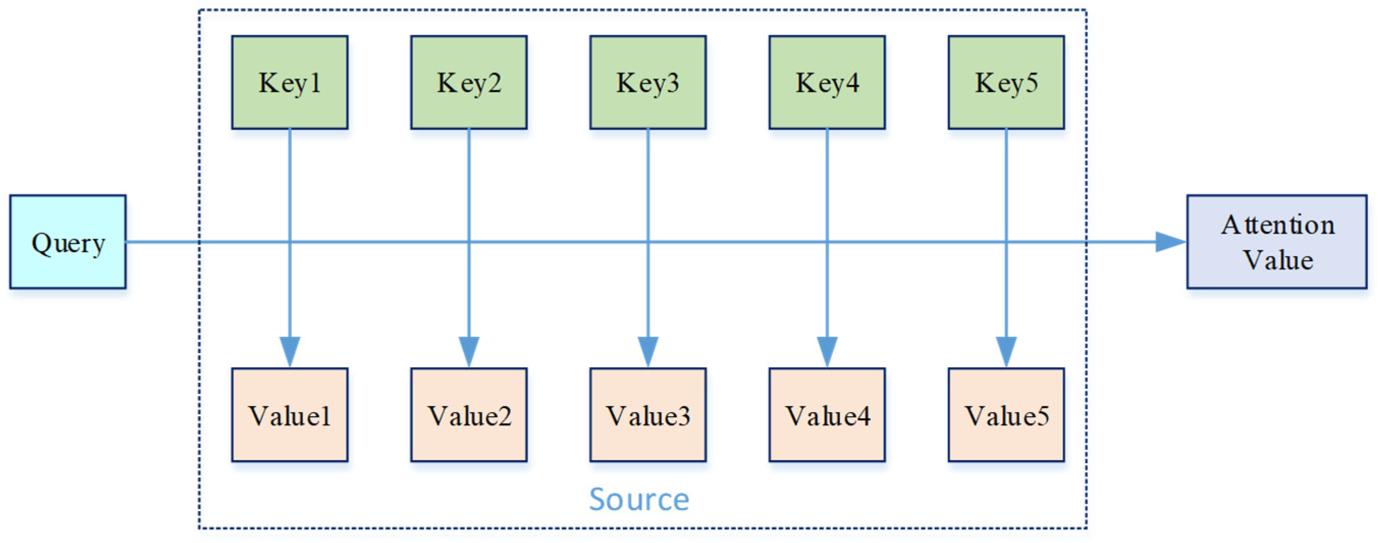
To better understand the attention mechanism, AM, it is extracted from the “encoder–decoding” framework, as shown in Figure 2:
As illustrated in Figure 2, when the input information is represented as key–value pairs, the entire source can be written as ( K 1 , V 1 ) , ( K 2 , V 2 ) , , ( K N , V N ) , where each “key” K i governs how much attention that piece of input should receive, and each “value” V i carries the actual content to be aggregated.
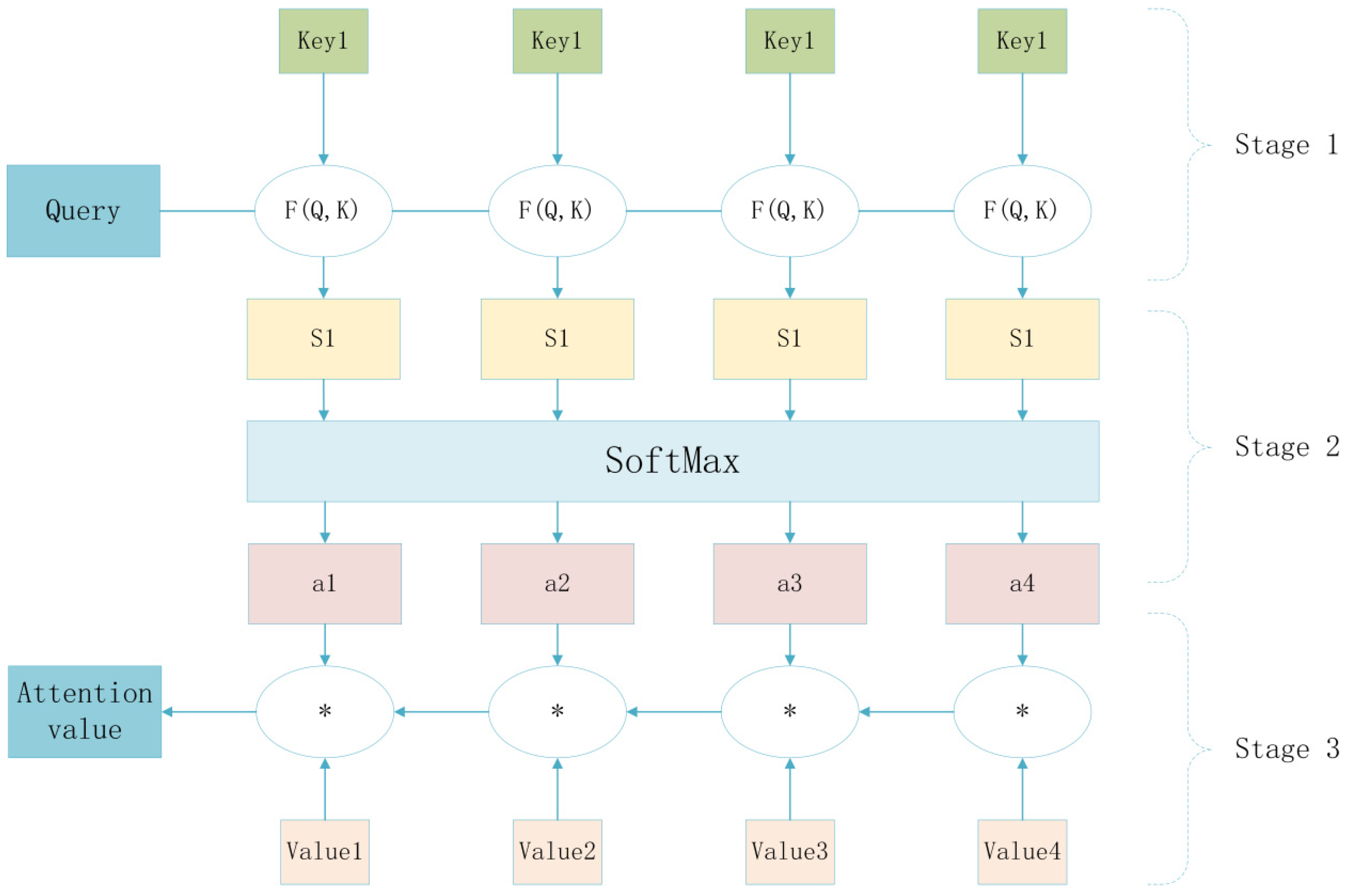
The calculation process of the AM can be summarized into three stages, as shown in Figure 3.
Stage 1: Calculate the relevance of the query and the key to get the attention score.
S i = F ( Q , K i )
The computational methods include dot product modeling, finding the cosine similarity, and additive modeling, as shown in Formulas (2)–(4).
S i ( Q , K i ) = Q K i
S i ( Q , K i ) = Q K i Q K i
S i ( Q , K i ) = V T tanh ( W Q + U K i )
where W, U, and V are learnable network parameters.
Stage 2: The correlations obtained in the first step are numerically transformed by SoftMax, as shown in Formula (5).
a i = s o f t max ( S i ) = e s i j = 1 N e s j
where a i is the corresponding weight coefficient of v a l u e i , and s is the similarity at the previous stage of the computation.
Stage 3: For a i and v a l u e i performing a weighted summation yields the attention value, as shown in Formula (6):
A t t e n t i o n ( ( K , V ) , Q ) = i = 1 N a i V a l u e i

3. Short-Term Wind Power Prediction Model with Multi-Layer Attention

3.1. A Description of the Multimodal Fusion Wind Power Prediction Problem

A subset of multimodal measurements from an offshore wind farm is used to illustrate six concurrent time series variables—the power output, wind speed, temperature, humidity, wind direction, and barometric pressure—collected over a specified interval.
The proposed network architecture incorporates a two-stage attention mechanism. In the first stage, a spatial attention module learns pairwise correlations among the input features at each time step, thereby highlighting the most informative sensors or variables. In the second stage, a temporal attention module selectively weights the spatially attended hidden representations across time to capture long-range dependencies. These temporally filtered states are then aggregated into context vectors that jointly encode spatial and temporal relationships. By alternating the spatial and temporal attention, the model effectively learns both inter-variable interactions at each instant and their evolution over extended horizons [26].
This article describes the prediction model problem of the multimodal fusion as follows:
We formulate the multimodal fusion prediction problem as follows. Given n ( n > 1 ) external time series X (including wind direction, temperature, etc.) and a target series Y (wind power), we denote these sequences and their variables as follows:
x ( k ) = ( x 1 k , x 2 k , , x T k ) T R T
The expression here represents the k -th external series over a window of length T, for k = 1 ,   2 , ,   5 . In our multimodal input, we take k = 1 to be the wind speed, k = 2 as the wind direction, k = 3 as the air pressure, k = 4 as the temperature, and k = 5 as the humidity so that
x = ( x 1 , x 2 , x 3 , x 4 , x ( 5 ) ) T
X = ( x 1 , x 2 , , x T ) T R 5 T
collects all five external series over the same window.
Y = ( y 1 , y 2 , , y T ) T R T
denotes the observed wind power output over the window.
Y ^ = ( y ^ T + 1 , y ^ T + 2 , , y ^ T + τ ) T R T
denotes the predicted values of the target series, where τ is the forecasting horizon.
Hence, given the historical external sequence x 1 , x 2 , , x T , x t R 5 , and the wind power history y 1 , y 2 , , y T , y t R , the τ -step-ahead wind power predictions Y ^ = ( y ^ T + 1 , y ^ T + 2 , , y ^ T + τ ) T are modeled by
y ^ T + 1 , y ^ T + 2 , , y ^ T + τ = F ( y 1 , y 2 , , y T , x 1 , x 2 , , x T )
where F(⋅) is the nonlinear mapping function to be learned.

3.2. Aerodynamic Characteristics and Mechanical Performance Analysis of Inflatable Savonius Wind Turbines

Today wind turbines are the primary equipment for harnessing wind energy. This article analyzes them from two perspectives: their aerodynamic characteristics and their mechanical performance. Starting from the aerodynamic characteristics of wind turbines, their output power can be written based on their characteristics [27]:
P o u t = 1 2 C p ( λ ) ρ D H V 3
λ = ω R V
where P o u t indicates the output power; C p ( λ ) represents the power factor, with typical peaks ranging from 0.15 to 0.25, the corresponding λ is between 0.8 and 1.2; ρ refers to the density of air; D stands for the diameter; H is the leaf height, V represents the incoming wind speed, λ represents the tip-speed ratio (TSR), ω is the angular velocity, and R is the radius.
The key factors influencing the wind turbine power output are the overlap ratio and the tip-speed ratio. The overlap ratio, defined as the horizontal overlap distance e between the two semi-cylindrical blades divided by the rotor diameter D, governs the startup torque: a larger e/D yields a higher initial torque at low wind speeds and lowers the cut-in speed. However, an excessive overlap also increases airflow leakage, reducing effective pressure during steady operation. Meanwhile, by adjusting the generator’s load—either electrically or mechanically—and maintaining the operation around the optimal tip-speed ratio, the electrical energy production can be maximized.
From the analysis of its mechanical performance, the equivalent inertia of its impeller J can be listed as follows:
J = m b l a d e R 2 2
E k = 1 2 J ω 2
where m b l a d e represents the mass of the impeller, and E k represents the kinetic energy of the rotating machinery. A larger moment of inertia requires greater wind force or more time to reach the operating speed, while a smaller moment of inertia allows the turbine to respond, accelerate, or decelerate more quickly to sudden wind speed changes (e.g., gusts). When wind speeds fluctuate, higher inertia stores more kinetic energy, smoothing out output variations. However, too much inertia compromises the system agility and adds structural weight. Thus, to maximize the power generation efficiency, these factors must be carefully balanced.

3.3. The General Framework of the Model

In this paper, we combine and reconfigure the attention mechanism and propose a short-term wind power prediction model based on the multi-layered attention mechanism and the bidirectional gating unit, BiGRU, with the multimodal fusion of the MAM-BiGRU, which adequately extracts the predicted power and the external sequences with the spatial and temporal factors. The overall framework of the MAM-BiGRU prediction model is shown in Figure 4.
The prediction model in this paper contains three stages:
Spatial modeling: We introduce a dual-stage spatial attention mechanism (DSAM) built upon a BiGRU backbone. The first layer of the DSAM captures local feature correlations among auxiliary time series inputs, while the second layer models their global relationships with the wind power output. By learning adaptive weights for each variable, the DSAM explicitly quantifies the contribution of every external measurement to the power generation.
Temporal modeling: A BiGRU-based temporal attention mechanism (TAM) is applied to the spatially attended representations. The TAM selectively emphasizes past hidden states that exhibit strong long-term dependencies and periodic patterns, enabling the network to learn both trend and seasonality effects inherent in multivariate wind power series.
Prediction output: The context vectors produced by the DSAM and TAM are concatenated with recent wind power observations and passed through a final BiGRU layer. This module generates the multi-step power output sequence, leveraging the fused spatio-temporal embeddings to enhance the prediction accuracy over extended horizons.

3.3.1. Hierarchical Struacture

To capture the spatial dependencies between auxiliary input sequences and the target power series, we propose a BiGRU-based, two-layer spatial attention mechanism (DSAM). The first sub-module (SAM1) attends exclusively to the external variables, extracting local inter-feature correlations and producing fine-grained attention weights. The second sub-module (SAM2) concatenates the wind power sequence with the SAM1-filtered representations, thereby learning their global spatial relationships and generating aggregated response weights. By stacking these two attention layers, the DSAM ensures a robust, comprehensive, and effective extraction of multivariate spatial features.
(1)
First layer of spatial attention mechanism SAM1
This layer of the attention module is used to extract the local spatial correlation between the external sequence data, and its model structure is shown in Figure 5:
Typically, given the k attribute vector of the external sequence ( x k ), attention weights can be calculated using α :
e t k = v f T Relu ( W f h t 1 f + U f x k + b f )
α t k = exp ( e t k ) j = 1 n exp ( e t j )
where Relu is the selected activation function, and v f ,   b f R T ,   W f R T × m ,   U f R T × T is the parameter to be learned. h t 1 f R m is the hidden state of the previous BiGRU unit, and m is the number of hidden cells in the BiGRU cell, the weighting of attention α determined by the historical hidden state and the current input, which represents the impact of each attribute on the prediction.
Since at each moment in time the individual sequence data have corresponding weights, the output of the first-stage spatial attention SAM1 can be expressed as follows:
x ~ t = ( α t 1 x t 1 , α t 2 x t 2 , , α t n x t n ) T
(2)
Second-level spatial attention mechanism SAM2
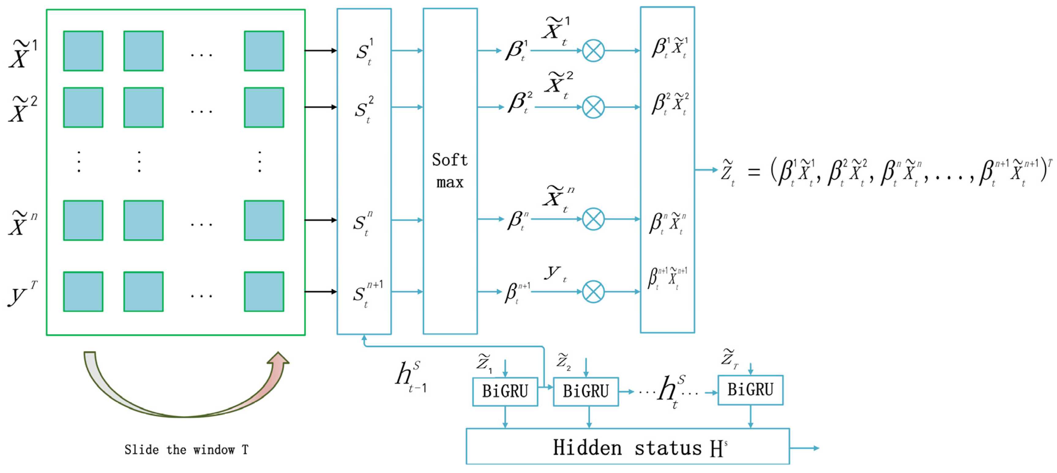
In this stage, the attention module is used to extract the global spatial correlation between the target sequence Y and the external sequence features, and its model structure is shown in Figure 6.
In this module, the y of the target sequence is spliced with the external sequence features x ~ t at the corresponding time to construct the vector z , z = [ x ~ ; y ] R ( n + 1 ) × T as the input data for this module. Then, the attention weight is calculated as follows:
s t k = v S T Relu ( W S h t 1 S + U S z + b S )
β t k = exp ( s t k ) j = 1 n + 1 exp ( s t j )
where Relu is the selected activation function, and v S ,   b S R T ,   W S R T × q ,   U S R T × T is the parameter to be learned. b t 1 S R q is the hidden state of the previous BiGRU cell, and q is the number of hidden cells in the BiGRU cell.
The output of the second level of the spatial attention SAM2 can be represented as follows:
z ~ t = ( β t 1 x t 1 , β t 2 x t 2 , , β t n + 1 x t n + 1 ) T

3.3.2. Time Attention TAM-BiGRU

Within the two-layer DSAM framework, spatial attention modules capture both inter-variable correlations among auxiliary inputs and their relationships with the power series over a fixed time window TTT, thereby learning some short-range temporal patterns. However, these limited temporal contexts may be insufficient for modeling longer-term dependencies. To remedy this, we introduce a BiGRU-based temporal attention module (TAM-BiGRU), whose architecture is illustrated in Figure 7.
For the i hidden state of the temporal attention, the attention weight of its temporal relation can be obtained through the attention mechanism γ :
d t i = v d T Relu ( W d h t 1 o + U d h i s + b d )
γ t k = exp ( d t i ) j = 1 T exp ( d t i )
where Relu is the selected activation function, and v d ,   b d R p ,   W d R p × p ,   U d R p × q is the parameter to be learned. h t 1 o R p is the hidden state of the previous BiGRU cell, and p is the number of hidden cells in the BiGRU cell. h i s H s denotes the i hidden state of the second layer of the spatial attention module SAM2.
Finally, the context vector c t at moment t represents the weighted summation of all hidden states, and the formula can be expressed as follows:
c t = k = 1 T γ t k h t o
Finally, the context vector c t and the hidden layer state of the BiGRU are used as the new hidden layer state, which is added to the fully connected layer and linearly transformed, and the final multi-step prediction result of the model is
y ^ T , y ^ T + 1 , , y ^ T + τ = ν y T ( W y [ o t ; c t ] + b y ) + b y
where W y R p 2 p and b y R τ reflect [ o t ; c t ] R 2 p to the hidden state of the decoder, v y R τ p is the model weight, and b y R τ p is the model bias.

4. Experimental Tests and Analysis of Results

The multimodal datasets for this study were drawn from two offshore wind farms on China’s southeastern coast, situated more than 100 km apart to minimize the overlap in regional environmental characteristics. Each dataset comprises six sensor streams—the power output, wind speed, wind direction, atmospheric pressure, ambient temperature, and humidity—recorded at 15 min intervals. The first dataset was used for the model training and validation, while the second, geographically independent dataset was employed to further assess the proposed model’s generalization capability across different offshore wind farm environments.

4.1. Experimental Design

Four different models, such as the GRU, BiGRU, TAM-BiGRU, and STAM-BiGRU, were used in the experiments to compare the MAM-BiGRU model proposed in this paper. Meanwhile, this experiment adopts the strategy of the recursive multi-step prediction for the multimodal wind power time series and establishes a sliding window for multivariate data to overshoot the short-term wind power prediction by 1–6 steps.
In this paper, the bidirectional function in the deep learning framework Keras 2.0.2 is chosen to create the BiGRU neural network layer. The specific setup of the MAM-BiGRU model proposed in this paper is shown in Table 1.

4.2. Experimental Results

In order to verify the effectiveness of the model proposed in this paper, four different models such as the GRU, BiGRU, TAM-BiGRU, and STAM-BiGRU are set up to compare the MAM-BiGRU model proposed in this paper, respectively. The experimental results, including LOSS training iteration plots, multi-step prediction result plots, and multi-step predictions, for each of the above five models are as follows.

4.2.1. Loss Function Training Iteration Plot

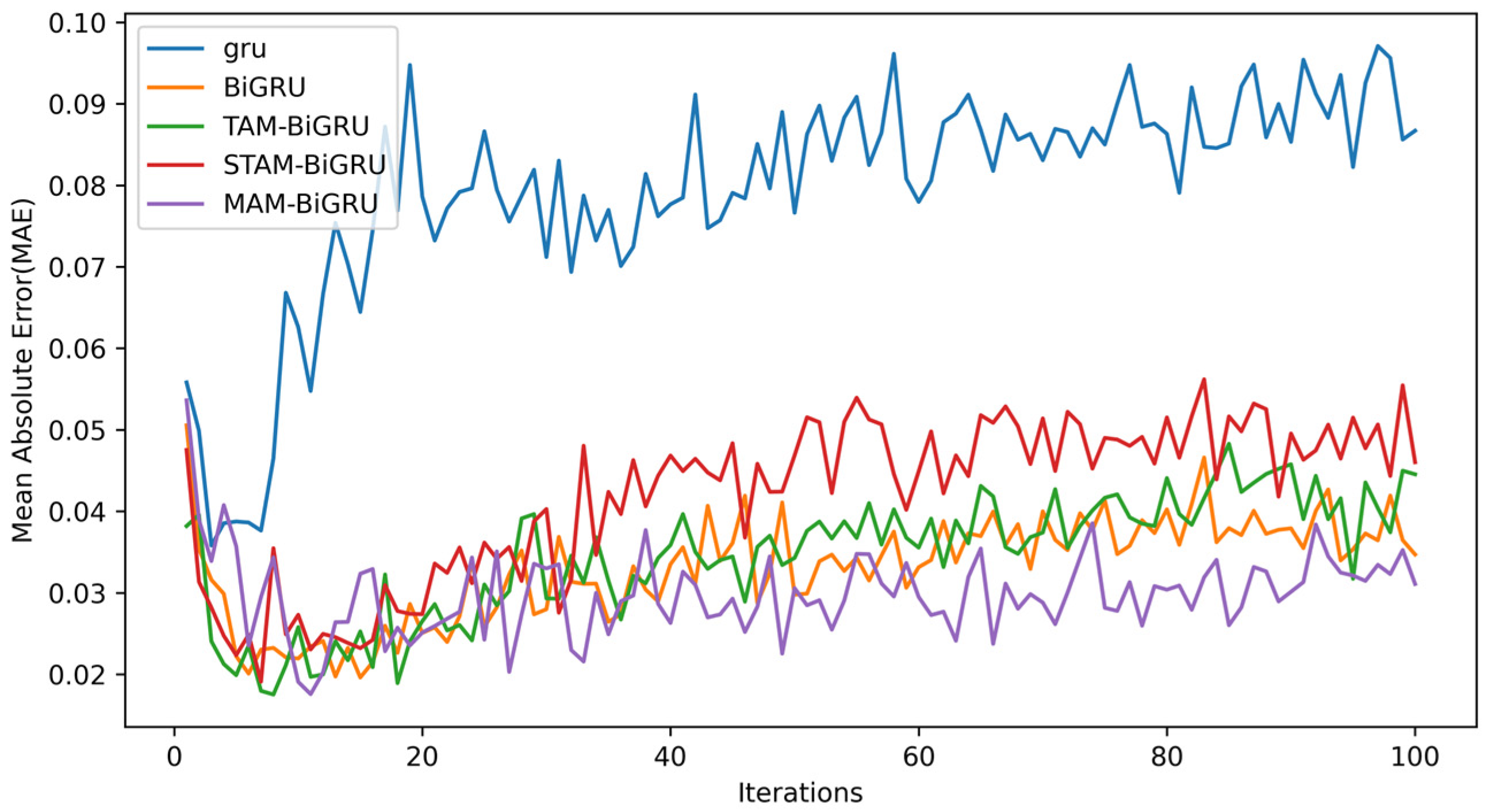
The loss function of each model is plotted using MAE training iterations as follows (Figure 8).
From Figure 8, it can be seen that the MAM-BiGRU model has a significant advantage in both the convergence speed and convergence accuracy, indicating that the model can learn the data well.

4.2.2. Plots of the Results of the Over-the-Top Multi-Step Prediction

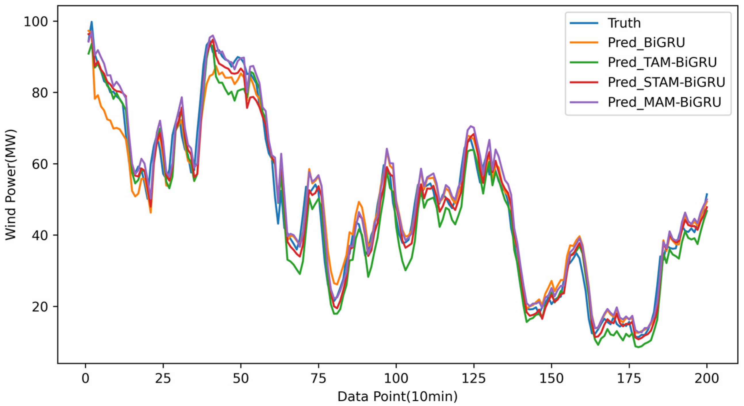
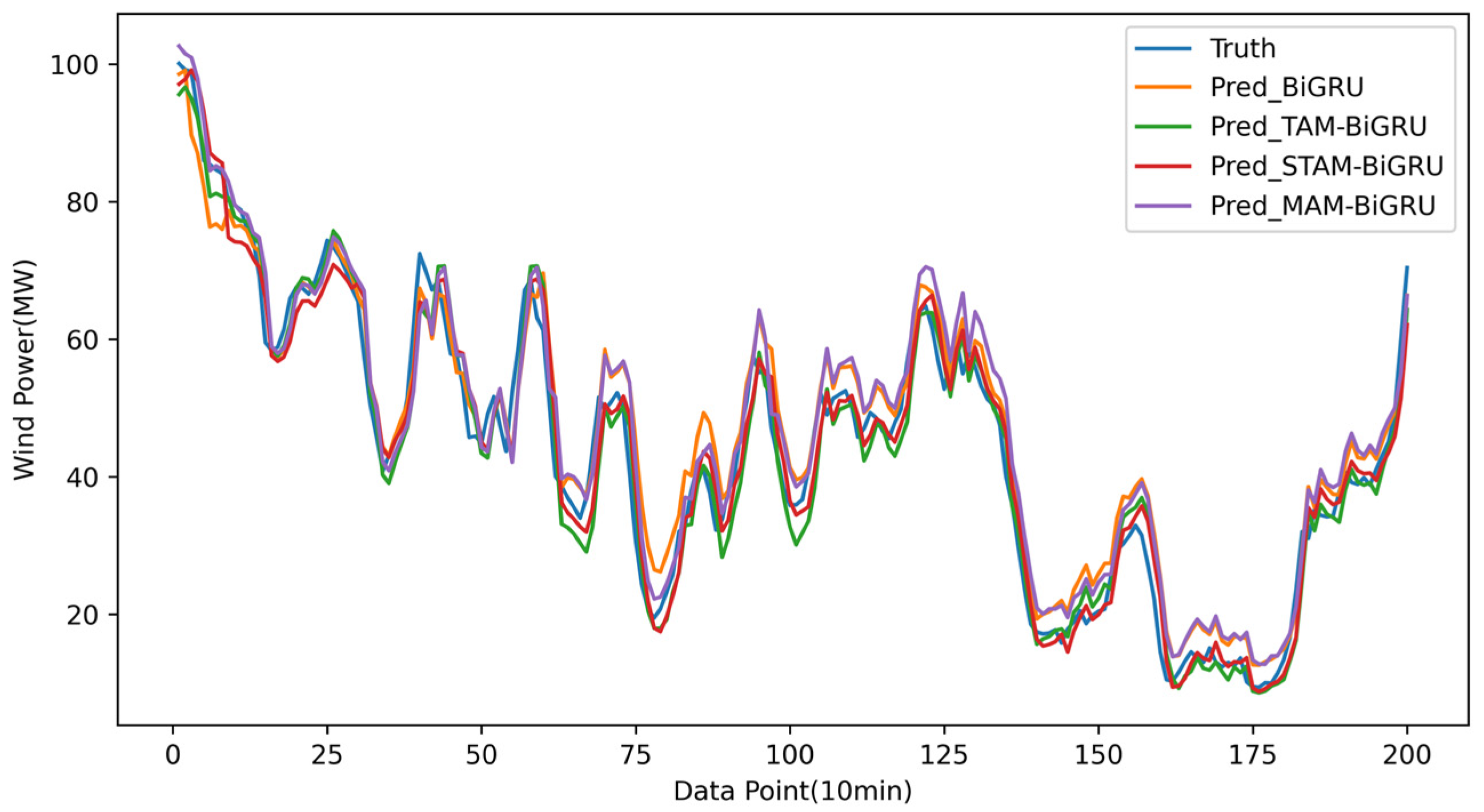
Comparison plots of the prediction results for multiple steps ahead (one, three, and five steps ahead) for each model are shown in Figure 9, Figure 10 and Figure 11.
The above figure shows that the predicted curves of the two models, the MAM-BiGRU and STAM-BiGRU, fit well with the actual power curve, while the curves predicted by the BiGRU and TAM-BiGRU are somewhat different from the original data.

4.2.3. Comparison Table of Prediction Accuracy of Models

Here, this paper evaluates the prediction accuracy of each model. The prediction error evaluation indexes of each model for multiple steps ahead on the first dataset are shown in Table 2 and Table 3, while those on the second dataset are presented in Table 4, which is used to illustrate the generalization ability of the model.
As can be seen from Table 2 and Table 3, the MAM-BiGRU exhibits a good prediction performance in multiple accuracy evaluation metrics for overshooting multiple steps. Meanwhile, the indicators in Table 4, which presents the prediction errors on the second geographically independent dataset, also demonstrate that the model has a good generalization ability.
This can be seen by analyzing the results of the ablation experiments described above:
  • Attention models are generally better: Models incorporating attention (MAM-BiGRU, STAM-BiGRU, TAM-BiGRU) consistently outperform vanilla GRU and BiGRU networks.
  • Temporal attention is effective but insufficient: While the TAM-BiGRU effectively captures long-term dependencies—yielding a higher accuracy than the GRU/BiGRU—it still neglects spatial interactions among input variables.
  • Limitations of single-layer spatio-temporal attention: The STAM-BiGRU improves short-term forecasts but degrades markedly over multi-step horizons, as its single spatial attention layer cannot fully model complex inter-variable relationships and is vulnerable to irrelevant feature noise.
  • Advantages of multi-layer spatio-temporal attention: The proposed MAM-BiGRU, with its stacked spatial and temporal attention modules, more comprehensively extracts multimodal features, preserves critical dependencies between the target and auxiliary sequences, and achieves the highest accuracy and stability in short-term multi-step predictions under complex offshore conditions.

5. Conclusions

In light of the limitations inherent in single-modality forecasting—where conventional models rely solely on power or wind speed series and thus neglect the interdependencies with multidimensional meteorological factors (e.g., temperature, barometric pressure, wind direction)—and given that the naïve aggregation of multimodal inputs can introduce redundancy and overfitting, we propose a novel fusion framework, the MAM-BiGRU. This architecture comprises two key components: (1) a double spatial attention module (DSAM), built on a bidirectional GRU, which learns both intra- and inter-modal spatial correlations to generate adaptive feature weights, and (2) a multi-layer temporal attention mechanism (TAM), also leveraging the BiGRU, which extracts long-term temporal dependencies and cyclic patterns. The experimental evaluation confirms that the MAM-BiGRU delivers superior forecasting accuracy and stability compared to benchmark methods.

Author Contributions

Conceptualization, Y.X.; methodology, Y.X.; software, X.G.; validation, Y.X., Y.L. and X.G.; formal analysis, S.L.; investigation, Y.X.; resources, Y.X.; data curation, X.G.; writing—original draft preparation, Y.L.; writing—review and editing, Y.L. and S.L.; visualization, S.L.; supervision, Y.X.; project administration, Y.X.; funding acquisition, Y.X. All authors have read and agreed to the published version of the manuscript.

Funding

This research was funded by the External Cooperation Program of Science and Technology Planning of Fujian Province (Grant No. 2022I0015) and supported by the Scientific Research Funds of Huaqiao University.

Data Availability Statement

The research data underlying these findings may be accessed by contacting yyxu@hqu.edu.cn with a reasonable request.

Conflicts of Interest

The authors declare no conflicts of interest.

Abbreviations

The following abbreviations are used in this manuscript:
AMAttention Mechanism
NWPNumerical Weather Prediction
ARAutoregressive
AIArtificial Intelligence
ANNArtificial Neural Network
BPNNBackpropagation Neural Network
ELMExtreme Learning Machine
WPDWavelet Packet Decomposition
LSTMLong Short-Term Memory Network
CNNConvolutional Neural Network
ARMAAutoregressive Moving Average
DWTDiscrete Wavelet Transform
EEMDEnsemble Empirical Mode
BABi-Attention Mechanism
CSOCrisscross Optimization Algorithm
MAMMulti-Layer Attention Mechanism
BiGRUBidirectional Gating Recurrent Unit
DSAMDual Spatial Attention Mechanism
TAMTemporal Attention Mechanism
RNNRecurrent Neural Network
GRUGating Recurrent Unit
STAMSpatio-Temporal Attention Mechanism
MAEMean Absolute Error
RMSERoot Mean Square Error
MSTAMMulti-Layer Spatio-Temporal Attention Mechanism

References

  1. Desalegn, B.; Gebeyehu, D.; Tamrat, B.; Tadiwose, T.; Lata, A. Onshore versus offshore wind power trends and recent study practices in modeling of wind turbines’ life-cycle impact assessments. Clean. Eng. Technol. 2023, 17, 100691. [Google Scholar] [CrossRef]
  2. Global Wind Energy Council. Global Wind Energy Council Report 2019. 2020. Available online: http://arxiv.org/abs/1704.02971 (accessed on 26 July 2025).
  3. Abdel-Aty, A.-H.; Nisar, K.S.; Alharbi, W.R.; Owyed, S.; Alsharif, M.H. Boosting wind turbine performance with advanced smart power prediction: Employing a hybrid AR–MA–LSTM technique. Alex. Eng. J. 2024, 96, 58–71. [Google Scholar] [CrossRef]
  4. de Castro, M.; Salvador, S.; Gómez-Gesteira, M.; Costoya, X.; Carvalho, D.; Sanz-Larruga, F.J.; Gimeno, L. Europe, China and the United States: Three different approaches to the development of offshore wind energy. Renew. Sustain. Energy Rev. 2019, 109, 55–70. [Google Scholar] [CrossRef]
  5. Lu, S.; Gao, Z.; Xu, Q.; Jiang, C.; Zhang, A.; Wang, X. Class-imbalance privacy-preserving federated learning for decentralized fault diagnosis with biometric authentication. IEEE Trans. Ind. Inform. 2022, 18, 9101–9111. [Google Scholar] [CrossRef]
  6. Li, M.; Jiang, X.; Carroll, J.; Negenborn, R.R. A multi-objective maintenance strategy optimization framework for offshore wind farms considering uncertainty. Appl. Energy 2022, 321, 119284. [Google Scholar] [CrossRef]
  7. Choi, Y.; Park, S.; Choi, J.; Lee, G.; Lee, M. Evaluating offshore wind power potential in the context of climate change and technological advancement: Insights from Republic of Korea. Renew. Sustain. Energy Rev. 2023, 183, 113497. [Google Scholar] [CrossRef]
  8. Hanifi, S.; Liu, X.; Lin, Z.; Lotfian, S. A critical review of wind power forecasting methods—Past, present and future. Energies 2020, 13, 3764. [Google Scholar] [CrossRef]
  9. Zhang, W.; He, Y.; Yang, S. A multi-step probability density prediction model based on Gaussian approximation of quantiles for offshore wind power. Renew. Energy 2023, 202, 992–1011. [Google Scholar] [CrossRef]
  10. Wu, Z.; Xia, X.; Xiao, L.; Liu, Y. Combined model with secondary decomposition-model selection and sample selection for multi-step wind power forecasting. Appl. Energy 2020, 261, 114345. [Google Scholar] [CrossRef]
  11. Poggi, P.; Muselli, M.; Notton, G.; Cristofari, C.; Louche, A. Forecasting and simulating wind speed in Corsica by using an auto-regressive model. Energy Convers. Manag. 2003, 44, 3177–3196. [Google Scholar] [CrossRef]
  12. Liu, H.; Tian, H.; Liang, X.; Li, Y. Wind speed forecasting approach using secondary decomposition algorithm and Elman neural networks. Appl. Energy 2015, 157, 183–194. [Google Scholar] [CrossRef]
  13. Rahimilarki, R.; Gao, Z.; Zhang, A.; Binns, R.R. Robust neural network fault estimation approach for nonlinear dynamic systems with applications to wind turbine systems. IEEE Trans. Ind. Inform. 2019, 15, 6302–6312. [Google Scholar] [CrossRef]
  14. Yan, L.; Hu, P.; Li, C.; Yao, Y.; Xing, L.; Lei, F.; Zhu, N. The performance prediction of ground source heat pump system based on monitoring data and data mining technology. Energy Build. 2016, 127, 1085–1095. [Google Scholar] [CrossRef]
  15. Zhao, Y.; Ye, L.; Li, Z.; Song, X.; Lang, Y.; Su, J. A novel bidirectional mechanism based on time series model for wind power forecasting. Appl. Energy 2016, 177, 793–803. [Google Scholar] [CrossRef]
  16. Yang, Z.; Wang, J. A hybrid forecasting approach applied in wind speed forecasting based on a data processing strategy and an optimized artificial intelligence algorithm. Energy 2018, 160, 87–100. [Google Scholar] [CrossRef]
  17. Lu, P.; Ye, L.; Zhao, Y.; Dai, B.; Pei, M.; Li, Z. Feature extraction of meteorological factors for wind power prediction based on variable weight combined method. Renew. Energy 2021, 179, 1925–1939. [Google Scholar] [CrossRef]
  18. Chen, H. Cluster-based ensemble learning for wind power modeling from meteorological wind data. Renew. Sustain. Energy Rev. 2022, 167, 112652. [Google Scholar] [CrossRef]
  19. Liu, H.; Yang, L.; Zhang, B.; Zhang, Z. A two-channel deep network based model for improving ultra-short-term prediction of wind power via utilizing multi-source data. Energy 2023, 283, 128510. [Google Scholar] [CrossRef]
  20. Hanifi, S.; Zare-Behtash, H.; Cammarano, A.; Lotfian, S. Offshore wind power forecasting based on WPD and optimised deep learning methods. Renew. Energy 2023, 218, 119241. [Google Scholar] [CrossRef]
  21. Qin, Y.; Song, D.; Chen, H.; Cheng, W.; Jiang, G.; Cottrell, G. A dual-stage attention-based recurrent neural network for time series prediction. arXiv 2017, arXiv:1704.02971. [Google Scholar]
  22. Meng, A.; Chen, S.; Ou, Z.; Ding, W.; Zhou, H.; Fan, J.; Yin, H. A hybrid deep learning architecture for wind power prediction based on bi-attention mechanism and crisscross optimization. Energy 2022, 238, 121795. [Google Scholar] [CrossRef]
  23. Wang, X.; Cai, X.; Li, Z. Ultra-short-term wind power forecasting method based on a cross LOF preprocessing algorithm and an attention mechanism. Power Syst. Prot. Control. 2020, 48, 92–99. [Google Scholar]
  24. Bahdanau, D.; Cho, K.; Bengio, Y. Neural machine translation by jointly learning to align and translate. In Proceedings of the International Conference on Learning Representations (ICLR), San Diego, CA, USA, 7–9 May 2015. Paper No. 1409.0473. [Google Scholar]
  25. Shi, Y.; Meng, J.; Wang, J. Seq2seq model with RNN attention for abstractive summarization. In Proceedings of the 2019 International Conference on Computational Linguistics & Intelligent Text Processing, Santa Fe, NM, USA, 10–16 April 2019. [Google Scholar]
  26. Yin, R.; Zhang, Y.; Zhou, X.; Wang, L.; Li, Q.; Chen, S. Time series computational prediction of vaccines for Influenza A H3N2 with recurrent neural networks. J. Bioinform. Comput. Biol. 2020, 18, 1023–1039. [Google Scholar] [CrossRef]
  27. Lin, J.; Wang, Y.; Yu, H.; Jian, L. Conceptual design of inflatable Savonius wind turbine and performance investigation of varying thickness and arc angle of blade. In Proceedings of the 2023 IEEE 7th Conference on Energy Internet and Energy System Integration (EI2), Hangzhou, China, 15–18 December 2023; pp. 1370–1376. [Google Scholar]
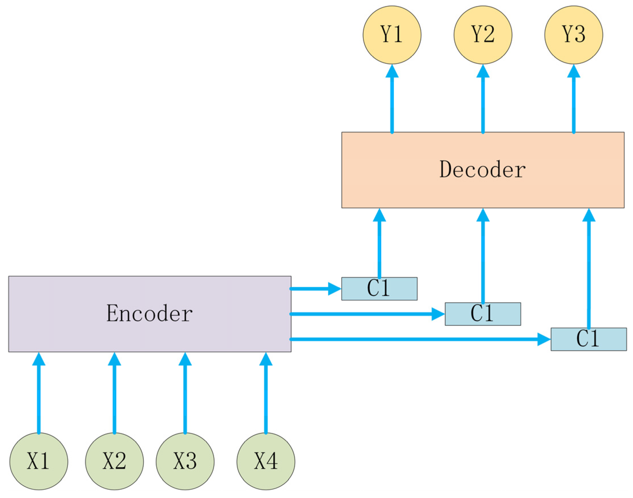
Figure 1. Extended encoder–decoder model diagram.
Electronics 14 03183 g001
Figure 2. Basic principle diagram of attention mechanism.
Electronics 14 03183 g002
Figure 3. The process chart of the attention mechanism computation.
Electronics 14 03183 g003
Figure 4. Overall framework of MAM-BiGRU prediction model.
Electronics 14 03183 g004
Figure 5. The structure of the first layer of the spatial attention mechanism model.
Electronics 14 03183 g005
Figure 6. The structure of the second layer of the spatial attention mechanism model.
Electronics 14 03183 g006
Figure 7. Structure of temporal attention mechanism model.
Electronics 14 03183 g007
Figure 8. Iterative validation error curve of MAE model.
Electronics 14 03183 g008
Figure 9. Comparison of one-step prediction results of different models.
Electronics 14 03183 g009
Figure 10. Comparison of three-step prediction results of different models.
Electronics 14 03183 g010
Figure 11. Comparison of five-step prediction results of different models.
Electronics 14 03183 g011
Table 1. Summary of MAM-BiGRU model parameter settings.
Parameter SymbolParameter Value
Input Dimension96 * 6
Time Steps96
BiGRU Layer Length64
BiGRU Activation FunctionRelu
Attention Dimension3
Batch Size64
Learning Rate0.0001
Epoch100
Dropout Prob0.3
Table 2. The table of prediction errors for each model on the first dataset (MAE).
Predicted Step SizeGRUBiGRUTAM-BiGRUSTAM-BiGRUMAM-BiGRU
Step 1 (15 min)0.02580.02530.02400.02370.0216
Step 3 (45 min)0.03160.03100.02940.02900.0265
Step 5 (75 min)0.05680.05570.05290.05210.0475
Step 8 (2 h)0.07910.07750.07360.07250.0659
Step 16 (4 h)0.08340.08170.07760.07650.0692
Step 32 (8 h)0.09050.08870.08430.08300.0757
Step 48 (12 h)0.09200.09020.08570.08440.0766
Step 96 (24 h)0.11210.10990.10440.10230.0932
Table 3. The table of prediction errors for each model on the first dataset (RMSE).
Predicted Step SizeGRUBiGRUTAM-BiGRUSTAM-BiGRUMAM-BiGRU
Step 1 (15 min)0.03150.03090.02930.02890.0264
Step 3 (45 min)0.03760.03680.03500.03450.0315
Step 5 (75 min)0.06230.06110.05800.05710.0520
Step 8 (2 h)0.07560.07410.07040.06930.0629
Step 16 (4 h)0.08290.08120.07960.07850.0697
Step 32 (8 h)0.09600.09410.08940.08800.0803
Step 48 (12 h)0.11760.11520.10950.10780.0979
Step 96 (24 h)0.13920.13640.12960.12520.1168
Table 4. The table of prediction errors for each model on the second dataset (MAE and RMSE).
Predicted Step SizeMAERMSE
GRUBiGRUMAM-BiGRUGRUBiGRUMAM-BiGRU
Step 1 (15 min)0.02540.02480.02380.03200.03070.0261
Step 3 (45 min)0.03130.03060.02920.03730.03700.0312
Step 5 (75 min)0.05730.05540.05340.06280.06090.0518
Step 8 (2 h)0.07890.07800.07330.07610.07390.0635
Step 16 (4 h)0.08390.08150.07820.08260.08170.0694
Step 32 (8 h)0.09010.08930.08480.09650.09380.0807
Step 48 (12 h)0.09260.08990.08540.011720.11580.0975
Step 96 (24 h)0.11180.11050.10410.13980.13610.1173
Disclaimer/Publisher’s Note: The statements, opinions and data contained in all publications are solely those of the individual author(s) and contributor(s) and not of MDPI and/or the editor(s). MDPI and/or the editor(s) disclaim responsibility for any injury to people or property resulting from any ideas, methods, instructions or products referred to in the content.