Ensemble-Based Knowledge Distillation for Identification of Childhood Pneumonia

Abstract

Childhood pneumonia remains a key cause of global morbidity and mortality, highlighting the need for accurate and efficient diagnostic tools. Ensemble methods have proven to be among the most successful approaches for identifying childhood pneumonia from chest X-ray images. However, deploying large, complex convolutional neural network models in resource-constrained environments presents challenges due to their high computational demands. Therefore, we propose a novel ensemble-based knowledge distillation method for identifying childhood pneumonia from X-ray images, which utilizes an ensemble of classification models to distill the knowledge to a more efficient student model. Experiments conducted on a chest X-ray dataset show that the distilled student model achieves comparable (statistically not significantly different) predictive performance to that of the Stochastic Gradient with Warm Restarts ensemble method (F1-score on average 0.95 vs. 0.96, respectively), while significantly reducing inference time and decreasing FLOPs by a factor of 6.5. Based on the obtained results, the proposed method highlights the potential of knowledge distillation to enhance the efficiency of complex methods, making them more suitable for utilization in environments with limited computational resources.

1. Introduction

Childhood pneumonia remains a significant global health challenge, responsible for over 700,000 deaths annually among children under five and accounting for approximately 14% of all deaths in this age group [1]. The burden is particularly high in developing regions such as South Asia, and West and Central Africa, where incidence rates reach up to 2500 and 1620 cases per 100,000 children, respectively, well above the global average of 1400 cases per 100,000 children [2]. Therefore, accurate and timely diagnosis is essential for effective treatment. However, in many low-resource settings, access to expert radiologic interpretation of chest X-ray images is limited, hindering prompt diagnosis and therapy [3].

Recent advancements in deep learning, especially with the utilization of convolutional neural networks (CNNs), have demonstrated high predictive performance in detecting various pathologies from medical images [4,5], including pneumonia [6,7], tubercolosis [8], and COVID-19 [9,10]. Such state-of-the-art models tend to be complex and computationally demanding, presenting challenges for their deployment in real-world, resource-constrained environments such as rural clinics or mobile health platforms [11]. Moreover, their computational complexity also increases vulnerability to adversarial attacks, posing serious risks in clinical practice [12]. Recent approaches, such as style contrastive learning [13], aim to mitigate these issues by learning representations prone to noise in data or imaging artifacts. While promising, these methods often rely on large-scale models and contrastive frameworks that remain computationally intensive, limiting their immediate applicability in real-world deployment scenarios. This concern further reinforces the motivation for developing models that are both computationally efficient and robust in real-world applications. Such approaches, in general, require substantial computational resources during the training phase, but on the other hand, often yield distilled neural network models with significantly lower inference time. This trade-off has led to an active line of research focused on developing lightweight and resilient architectures, particularly for the purpose of deployment in resource-constrained settings. From the perspective of efficient and sustainable neural network model deployment, such approaches align with the principles of Green AI [14].

To address these challenges, various strategies and methods were developed, including model pruning [15], quantization [16], and low-rank factorization [17]. While effective in reducing model size and inference latency, these methods often require post hoc tuning and may result in degraded predictive performance. Among these, knowledge distillation (KD) has emerged as an auspicious approach [18]. In the process of KD, a smaller, “student” model learns to replicate the behavior of a larger, computationally complex “teacher” model without significant loss in predictive performance [18]. Knowledge distillation techniques have been applied to reduce the complexity of neural networks for detecting diseases in various medical image analysis tasks [19], such as COVID-19, pneumonia, and tuberculosis from chest X-rays [20], facilitating their use in automated medical applications [21].

A common limitation across previous efforts is their reliance on a single teacher model, which can restrict the diversity of knowledge transferred to the student and may limit generalizability in complex diagnostic tasks. To address this, the use of multiple teacher models has gained attention [22,23]. The problem of utilizing a multiple teachers approach in the process of knowledge distillation is the significant amount of computational complexity needed to obtain a diverse group of models, since it is required in order to train multiple, usually deep, neural network architectures, which limit their practical applicability. However, in the past, ensemble methods [7,24,25,26] have demonstrated great predictive performance and are capable of creating a diverse group of ensemble models, often without significantly increasing computational complexity in the training phase. Therefore, we propose an ensemble knowledge distillation method (EKD) which uses a selection of top-performing ensemble models as teachers in the process of distilling their knowledge into a single student model, with the goal of maintaining predictive performance and ability to generalize, while significantly reducing computational complexity in the inference time. The predictive and inference performance of the proposed EDK method is evaluated for the task of identifying childhood pneumonia from chest X-ray images. The main contribution of our research is as follows:

• We propose an ensemble knowledge distillation method for image classification, utilizing multiple teacher models obtained from the SGDRE method. This approach reduces the distilled student model’s complexity and computational demands.

This main contribution is further supported by the following:

• A comprehensive empirical evaluation of the presented EKD method is conducted, addressing the task of identifying childhood pneumonia from chest X-ray images.
• An in-depth analysis and comparison are performed to assess the predictive performance and computational complexity of the distilled student model relative to both the SGDRE method and a conventionally trained student model.

The remainder of this paper is structured as follows. Section 2 presents the methods and materials used. Section 3 describes the experimental setup, including evaluation methods and metrics. Section 4 presents the experimental results in detail, followed by a discussion in Section 5. Finally, Section 6 concludes the study by summarizing the presented work and highlighting potential future work.

2. Related Work

In recent years, numerous studies have explored KD for improving the computational efficiency of deep neural networks, particularly in medical imaging applications. In the context of chest X-rays, KD has proven effective for compressing complex networks while preserving performance [20,21]. For example, KD has been employed to distill knowledge from large networks trained on expert-labeled datasets to smaller models designed for edge deployment in disease classification and segmentation tasks [19].

Several recent studies have further refined the KD process. Prototype-based knowledge distillation methods have been proposed to tackle challenges in medical segmentation, particularly when only single-modal data is available [27]. Such approaches aim to transfer semantic structures through compact class representations. For instance, Wang et al. [27] proposed a prototype knowledge distillation approach that transfers intra-class and inter-class feature variations from a multi-modal teacher to a single-modal student, enhancing segmentation performance even when only single-modal data is available. In a recent study [28], Asham et al. propose a lightweight deep learning model leveraging optimizing KD process by training multiple candidate teacher models and finding the most suitable one. Galih et al. [29] proposed an approach which employs the Vision Transformer (ViT) architecture as the teacher model and MobileNet as the student model in order to reduce computational complexity of student model. To achieve the same goal, Ghosh in their study [30] proposed a KD approach where models pretrained on the ImageNet dataset serve as teacher models. Additionally, Bi et al. [31] developed a Multi-Prototype Embedding Refinement method for semi-supervised medical image segmentation, capturing intra-class variations by clustering voxel embeddings along multiple prototypes per class. Such methods demonstrate the potential of using representative and interpretable feature structures to enhance model learning efficiency and generalization.

However, a common limitation across these efforts is the reliance on a single teacher model. This can restrict the diversity of knowledge transferred to the student and may limit generalizability in complex diagnostic tasks. To address this, the use of multiple teachers has gained attention [22,23,32]. This approach allows the student model to learn from a more diverse ensemble of teacher models, potentially capturing complementary information. For example, Li et al. [32] proposed a dual online knowledge distillation strategy to connect heterogenous networks with the developed multi-scale feature refinement module and thus transfer the knowledge from different sources. Cheng et al. [23] proposed an approach that integrates both localized and globalized frequency attention techniques, aiming to substantially enhance the distillation process. Additionally, Fukuda et al. [22] employed a KD approach using multiple models, including very deep networks and Long Short-Term Memory (LSTM) models, to train a standard CNN model, demonstrating the versatility of the KD process.

However, a common problem of utilizing a multiple teachers approach in the process of knowledge distillation is the significant computational complexity needed to obtain a diverse group of models, since it is required in order to train multiple, usually deep, neural network architectures, which limits their practical applicability. In contrast to aforementioned approaches, our proposed EKD method utilizes the SGDRE method for the purpose of obtaining multiple teacher models in the single training process and thus reducing computational complexity.

3. Materials and Methods

3.1. Knowledge Distillation

Knowledge distillation (KD) is the process of transferring knowledge from a large, computationally complex model, usually a deep neural network, to a smaller, more efficient model that retains comparable predictive performance while being computationally feasible for deployment in more resource-constrained environments. The inspiration behind the idea was drawn from natural processes, particularly biological metamorphosis, in which many insects, such as butterflies, undergo two distinct life stages optimized for different functions. Larval stage is optimized for consuming resources and growing, which is an analogy for training large complex models, and adult stage is optimized for efficiency, mobility, and reproduction, like the predictive models should be when feasible for deployment.

The principle behind knowledge distillation is based on utilizing soft labels—the teacher model’s output actions (logits)—as opposed to utilizing definite class labels only, to train the student models. These soft labels convey additional information regarding the inter-class relationships that are not present in the one-hot encoded ground truth labels. Formally, given an input x, a teacher model with parameters ${\theta }_T$ produces output signal $z_T=f_{{\theta }_T}\left(x\right)$. Similarly, a student model with parameters ${\theta }_S$ produces output signal $z_S=f_{{\theta }_S}\left(x\right)$.

The knowledge transfer is achieved by introducing a temperature parameter T in the softmax function to generate soft probability distributions:

$$p_i^T\left(x\right)={\displaystyle \frac{exp(z_{T,i}/T)}{{\sum }_{j}exp(z_{T,j}/T)}}$$

$$p_i^S\left(x\right)={\displaystyle \frac{exp(z_{S,i}/T)}{{\sum }_{j}exp(z_{S,j}/T)}}$$

where $p_i^T\left(x\right)$ and $p_i^S\left(x\right)$ can be interpreted as probabilities of class i for input x from the teacher and student models, respectively. The temperature parameter T controls the softness of the probability distribution. When $T=1$, we obtain the standard softmax outputs. As T increases, the probability distribution becomes more uniform, placing more weight on the relative relations between classes.

The student model is then trained to optimize a combined loss function:

$$\mathcal{L}\left({\theta }_S\right)=\alpha {\mathcal{L}}_{CE}(y,\sigma \left(z_S\right))+(1-\alpha ){\mathcal{L}}_{KD}(p^T,p^S)$$

where ${\mathcal{L}}_{CE}$ is the standard cross-entropy loss between the one-hot encoded ground truth labels y and the student’s predictions with a standard softmax $\sigma (·)$. ${\mathcal{L}}_{KD}$ is the knowledge distillation loss, typically implemented as the Kullback–Leibler (KL) divergence between the teacher’s and student’s soft probability distributions.

Advancements in knowledge distillation have expanded beyond the original formulation, one of which is transferring not only the outputs but also the intermediate representation [33]. Additionally, distilling knowledge from an ensemble of teacher models into a single student model [34,35] is also gaining attention in recent years.

3.2. SGDRE Method

Stochastic gradient descent (SGD) with warm restarts (SGDRE) [7] is an ensemble method that periodically resets the learning rate of the SGD optimized to encourage convergence to the local minima. Building upon this idea, the SGDRE method constructs an ensemble of models from a single training run by capturing multiple model snapshots at different restart points using the warm restarts mechanism. These snapshots, representing models converged to different local optima, are then used collectively as teacher models to transfer diverse knowledge to the student model during the knowledge distillation process. The conceptual design of the method is depicted in Figure 1. The SGDRE method results in enhanced performance for image classification tasks, particularly in the context of medical image analysis.

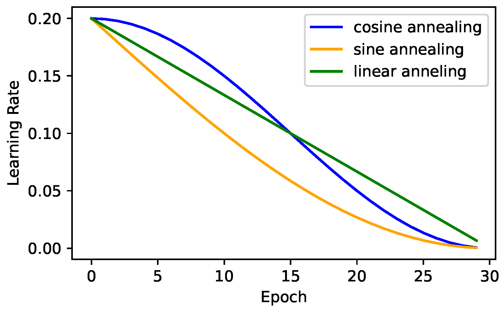
The key improvement introduced in this study lies in the modification of the training process, where, in contrast to conventional practice, in which the learning rate is gradually decreased through the training process, here the learning rate is periodically increased with the utilization of SGD with warm restarts. The SGD with warm restarts mechanism was initially presented in [36]. The main goal of this mechanism was to address the main SGD issue, which is that it is likely to converge prematurely, which can result in inferior solutions, especially in the case of deep neural network architectures. The SGDRE method uses the aforementioned mechanism with three different learning rate annealing strategies presented in Figure 2, to obtain a diverse set of candidate ensemble models through one training process.

As can be observed in Figure 1, the method consists of three training phases. The whole training process is designed to efficiently work under the limited training budget—limited number of epochs. In the initial training phase, the SGDRE is trained with the SGD optimizer, linearly reducing the initial learning rate for 50 epochs. After the initial training phase, the SGD learning rate is increased to 0.01 and 0.02, employing the sine decrease of the learning rate and early stopping mechanism, monitoring the area under the ROC curve (AUC) metric, which is calculated after each training epoch. The process of increasing the learning rate is then repeated with the only difference being the utilization of a cosine learning rate decay; however, the starting point of this process remains the same, after the initial training phase. Each warm restart is budgeted with an equal number of epochs, which is calculated based on the initial training budget subtracted by the epochs consumed in the initial training phase. Such a process of employing warm restarts with different initial learning rates and annealing strategies encourages a broader exploration of the loss surface, to uncover potentially more diverse and higher-quality solutions, and can also help improve generalization performance. The models obtained in this process are then evaluated. The top three individually best-performing models based on AUC scores are selected for the purpose of the ensemble method. The predictions of selected models are combined using the averaging approach, and the computed average finally serves as a final ensemble prediction.

In the original SGDRE study [7], the CNN architecture proposed by Stephen et al. [37] was utilized, which has already been demonstrated to be successful at solving the classification task to identify pneumonia based on the X-ray images. The architecture is composed of four convolutional layers (with 32, 64, and two with 128 filters) paired with max-pooling layers, followed by a flatten layer, a dropout layer (dropout rate 0.5), and two fully connected layers (with 512 and 1 neurons). All convolutional layers use $3\times 3$ kernels with ReLU activation. The proposed CNN architecture results in 6,795,394 trainable parameters.

3.3. Ensemble Knowledge Distillation

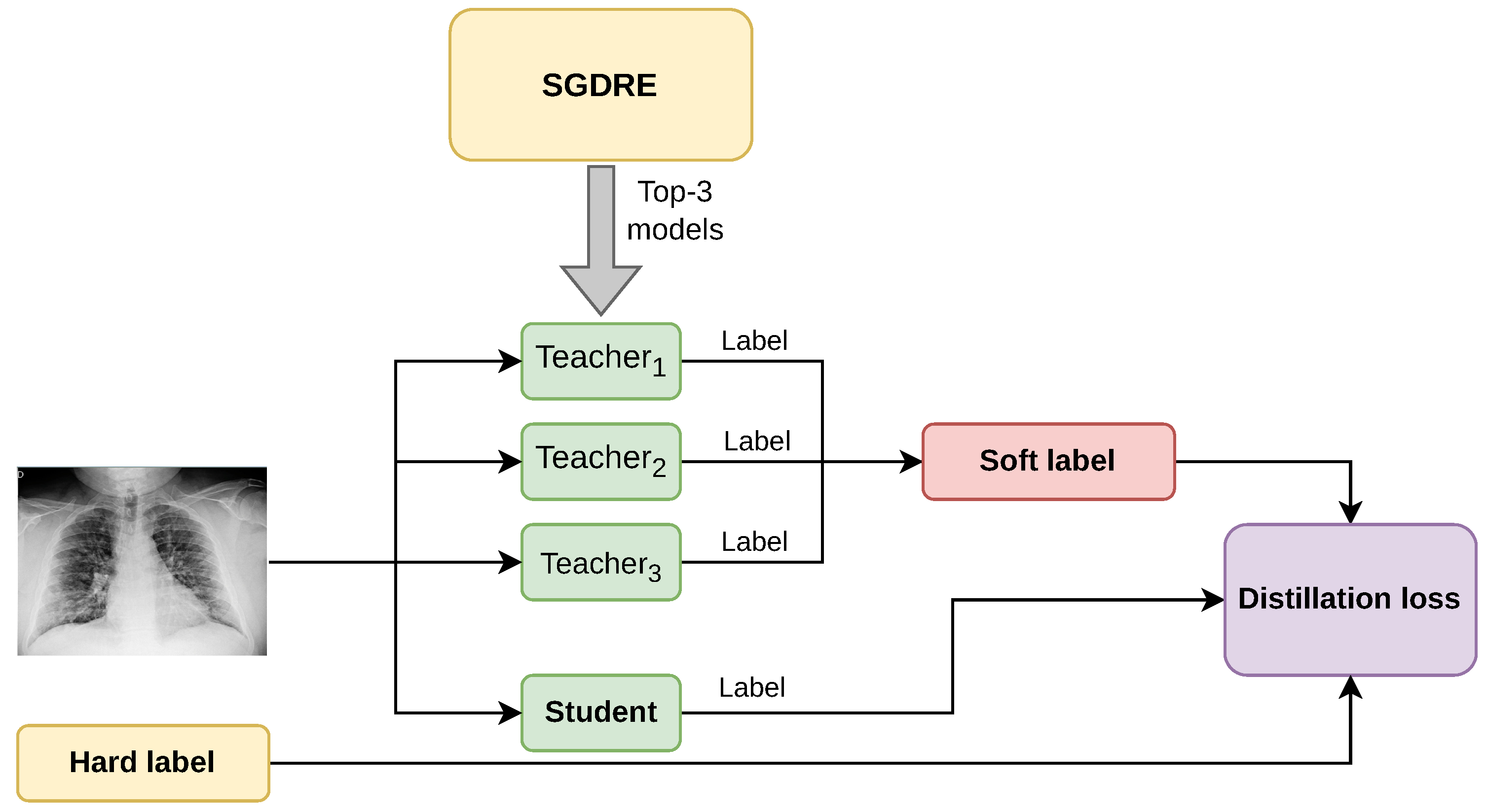
Based on the presented SGDRE method, we propose an ensemble-based knowledge distillation method, EKD, for the task of identifying childhood pneumonia from chest X-ray images. The method leverages multiple teacher models to distill the knowledge into a more compact student model. The process involves training an SGDRE method from which we obtain ensemble models that achieved acceptable performance and distilling their knowledge into a single student model. The conceptual diagram of the method is presented in Figure 3.

From the SGDRE method, we obtain the top three best-performing models, which are selected based on the AUC metric. Although the models output class probabilities via the softmax layer, we calculate AUC in a one-vs-rest manner by treating the softmax score for each class as a continuous-valued prediction. After the selection, the three teacher models are in the process of training, utilized for the purpose of distilling the knowledge through the computed soft label. Soft label combines the predicted labels of each teacher model into one unified label. Given an input sample x, the probability distribution predicted by each of the teacher models is calculated as:

$$p_k\left(y\right|x)=\sigma (z_k/T)$$

(1)

where $z_k$ denotes the logits produced by the k-th teacher model and $\sigma$ denotes the softmax function. The teachers’ combined soft label $p_{soft}$ is then calculated as the average of all teachers’ predictions:

$$p_{soft}\left(y\right|x)={\displaystyle \frac{1}{K}}\sum _{k=1}^K{p}_k\left(y\right|x)$$

(2)

In such a manner, the calculated soft labels reflect the diversity of multiple teacher models, capturing richer information than hard labels. The calculated soft label, together with the predicted label from the student model, and the ground-truth hard label, are afterward combined into the distillation loss value. The composite distillation loss value balances the true label loss and the soft label loss, and can be formally expressed as:

$${\mathcal{L}}_{KD}=\alpha ·{\mathcal{L}}_{CE}(y,\mathrm{softmax}\left(\widehat{z}\right))+(1-\alpha )·T^2·{\mathcal{L}}_{CE}(p_{\mathrm{soft}},\sigma (\widehat{z}/T))$$

(3)

where ${\mathcal{L}}_{CE}$ is the categorical cross-entropy loss, y denotes the ground truth labels, $\widehat{z}$ represents the student model’s logits, T is the temperature parameter which controls the probability distribution during the loss computation, and $\alpha$ is a weighting factor balancing both $p_{soft}$ loss and true label loss. The factor $T^2$ is included to preserve the relative contributions of the soft targets during training. The distillation loss value calculated in such a manner is further used in the process of training the student model, serving as the loss metric.

3.4. Dataset

The Chest X-ray images dataset is a publicly available dataset [38], originally collected and presented by Kermany et al. [39]. Chest X-ray images were collected from retrospective cohorts of pediatric patients aged 1 to 5 years from Guangzhou Women and Children’s Medical Center, Guangzhou, China. After the process of collecting the images, each image went through a rigorous process of quality control, removing all low-quality or unreliable scans. Finally, two expert physicians were utilized in grading the diagnoses of chest X-ray images prior to them being approved for use in the process of training the CNN [38].

In the preprocessing phase, we have resized the original X-ray images, which have different sizes, to a uniform size of 200 × 200 pixels. The total number of samples in the data set is 5858, which is unevenly distributed between the two classes. The “normal” class includes the X-ray images that do not show signs of pneumonia, and the “pneumonia” class contains the X-ray images that are diagnosed with pneumonia. The distribution between the classes can be observed in Figure 4. We can see class imbalance where the pneumonia-diagnosed images represent 72.96% of all the image samples, and the remaining 27.04% X-ray images of normal lungs.

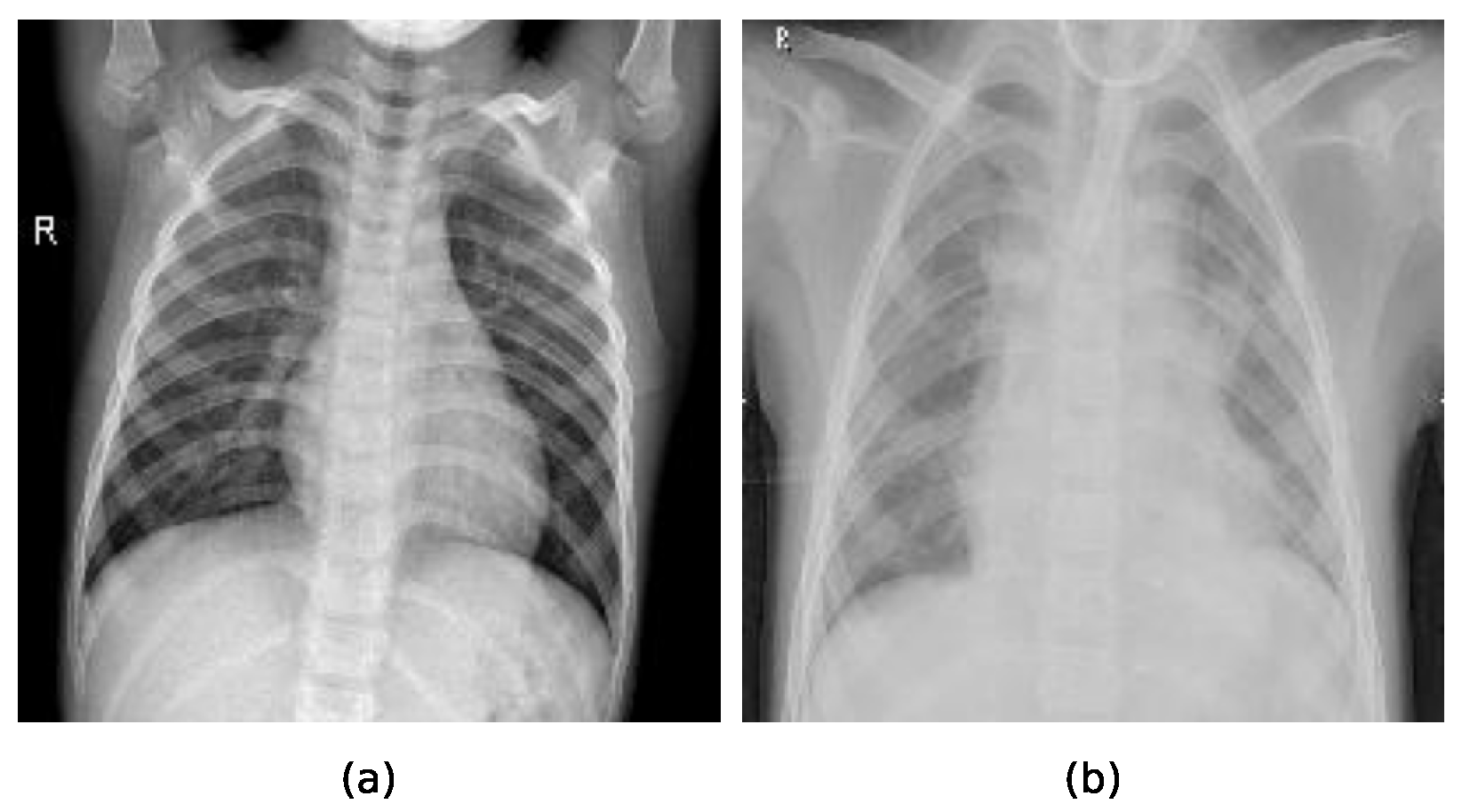
Two sample chest X-ray images used for training and evaluation of the compared methods can be observed in Figure 5, where the sample a represents the X-ray image of a healthy lung, while the sample b represents the X-ray image of lungs indicating pneumonia.

4. Experimental Framework

The proposed method for knowledge distillation from ensemble models to a single student model was evaluated on the task of childhood pneumonia identification based on the X-ray images. To objectively evaluate the performance of the proposed ensemble knowledge distillation method, EKD, we compared its performance with that of the ensemble method. Additionally, we conducted an experiment where we conventionally trained the student CNN architecture using randomly initialized weights in order to determine whether the utilization of the proposed method is justified. Therefore, in total, we conducted four experiments:

• Trained student CNN architecture in a conventional manner. The method is denoted as Student.
• Trained the SGDRE method, denoted as a SGDRE.
• Trained the proposed ensemble knowledge distillation method, utilizing the teacher models obtained by the SGDRE method, denoted as EKD.
• Trained the student model using knowledge distillation utilizing only one teacher from SGDRE method, denoted as KD.

All experiments were conducted on a computer with an octa-core Intel i7-6700 processor, 16 GB of RAM, and an Nvidia GeForce GTX 1660 Ti with 6 GB of memory, running on the Linux Mint 6 Debian edition operating system.

The following subsections present the evaluation method and metrics, the utilized student CNN architecture, and parameter settings for each of the conducted experiments.

4.1. Evaluation Methods and Metrics

We adopted a well-established 10-fold cross-validation approach as suggested by Demšar et al. [40], to assess the predictive performance of the predictive models produced by the proposed ensemble knowledge distillation method for identification of childhood pneumonia. This approach involves partitioning the dataset into ten equal subsets. In each iteration, nine subsets are used for training of the method, while the remaining subset serves as the test set. In such a manner, the process is repeated ten times, with each subset once serving as the test set. With 10-fold cross-validation, we mitigate variance by averaging over multiple data partitions and ensure that the model’s performance is not overly dependent on a particular data partition. The predictive performances of the compared methods are evaluated through common classification metrics such as accuracy, F1 score, AUC, and Cohen’s kappa score. Additionally, we captured the training time, the number of epochs consumed, and the inference time to inspect and analyze the performance from a computational complexity standpoint.

The accuracy metric is one the most commonly used metrics for evaluating the performance of classification algorithms [40]. It represents the proportion of correct predictions out of the total number of predictions. Formally, we can express the accuracy metric as:

$$\mathit{Accuracy}={\displaystyle \frac{TP+TN}{TP+TN+FP+FN}}$$

(4)

where $TP$ are correctly classified positive instances, $TN$ are correctly classified negative instances, $FP$ are negative instances incorrectly classified as positive, and $FN$ are positive instances incorrectly classified as negative.

Since the accuracy metric can be misleading, especially when dealing with unbalanced datasets, it is common to use the F1-score [41] metric, which is often used in such scenarios. It represents the harmonic mean of the precision and recall, balancing the trade-offs between those two metrics. We can formally express the F1-score metric as:

$$F1-\mathit{score}=2\times {\displaystyle \frac{P\times R}{P+R}}$$

(5)

where P denotes the precision metric, which can be expressed as

$$P={\displaystyle \frac{TP}{TP+FP}}$$

(6)

and R denotes the recall metric formally expressed as

$$R={\displaystyle \frac{TP}{TP+FN}}.$$

(7)

The area under the curve (AUC) metric is also widely used to evaluate the discriminatory ability of classifiers [42]. It measures the area under the receiver operating characteristic (ROC) curve, while ROC is defined as the true positive rate (TPR), against the false positive rate (FPR) across various values of a classification threshold. The AUC represents the probability that the classifier will assign a higher score to a randomly chosen positive instance than to a randomly chosen negative one. The classifier’s performance is then summarized across all possible threshold values, thus forming a family of classifiers parameterized by the decision threshold. In this context, the parameter is the classification threshold, which is used to convert the model’s continuous output scores into binary predictions. By varying this threshold, a family of thresholded classifiers is created, each with different TP rate and FP rate values. The AUC metric can be formally expressed as:

$${\int }_0^{1}TPR\left(\theta \right)dFPR\left(\theta \right)$$

(8)

where m denotes the model and $\theta$ denotes the classification threshold.

Cohen’s kappa [43] is a statistical measure developed initially to quantify inter-rater agreement, but it is also widely used to evaluate the level of agreement between a classifier’s predicted class and the ground truth class. It compares an observed accuracy to an expected accuracy (chance), while taking into account random chance, which generally makes it less misleading than simply using accuracy as a metric. Formally, the Cohen’s kappa metric can be expressed as:

$$\kappa ={\displaystyle \frac{p_o-p_e}{1-p_e}}$$

(9)

where $p_o$ is the relative observed agreement among raters, and $p_e$ is the hypothetical probability of chance agreement. The interpretation of the metric values depends on several definitions, one being proposed by Landis and Koch [44] in which they described the values <0 as no agreement, 0–0.20 as slight, 0.21–0.40 as fair, 0.41–0.60 as moderate, 0.61–0.80 as substantial, and 0.81–1 as almost perfect agreement.

4.2. Student CNN Architecture

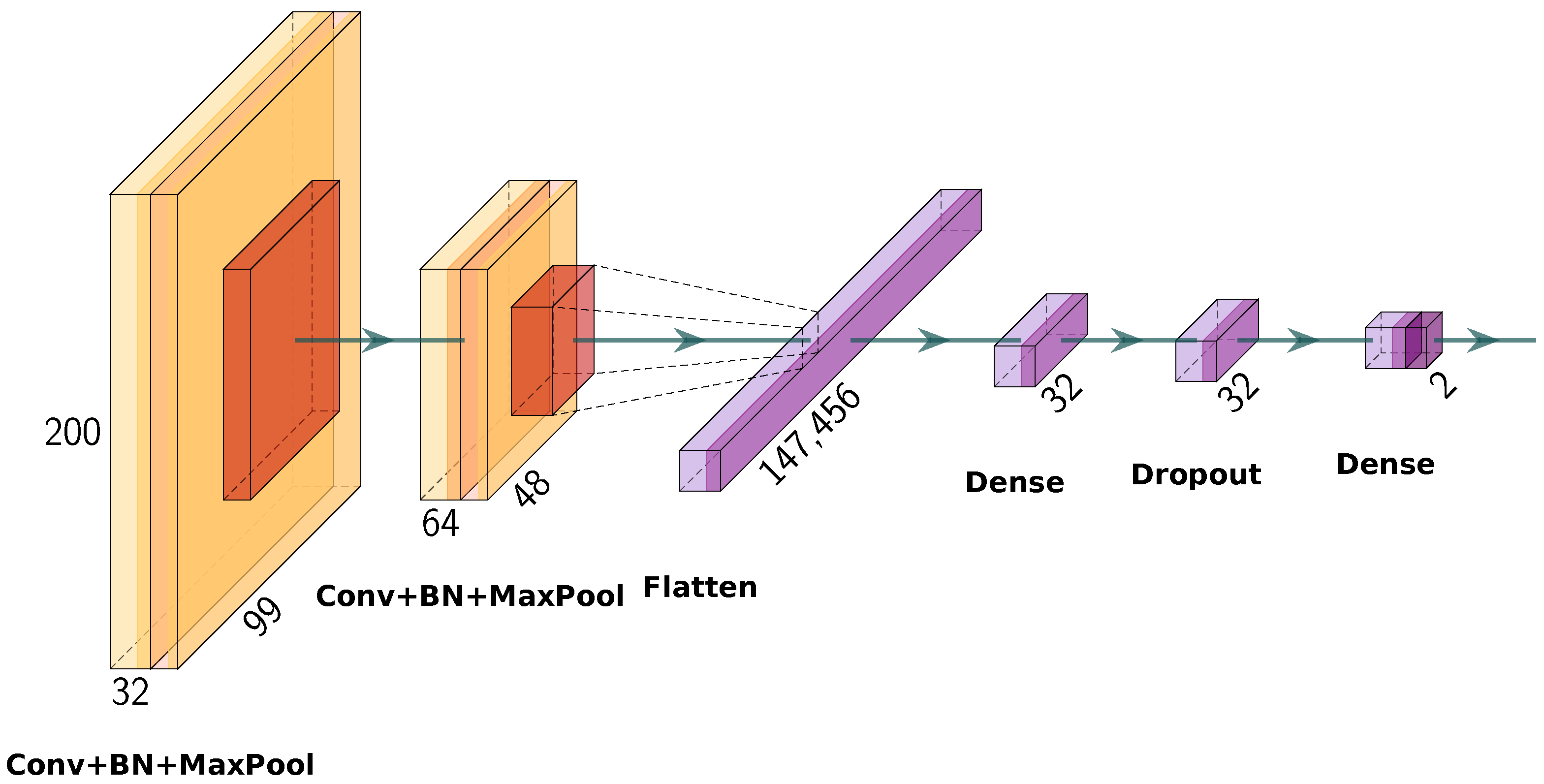
The architecture of the student CNN, graphically presented in Figure 6, is based on the architecture presented by Stephen et al. [37]. However, we modified it to facilitate effective feature extraction and classification with a minimalistic structure. The architecture comprises a serial combination of convolutional layers, normalization layers, pooling layers, and fully connected layers. The input to the network is a $200\times 200\times 1$ grayscale X-ray image. The first convolutional layer applies 32 filters of size $3\times 3$ with ReLU [45] activation function and Glorot uniform [46] weight initialization, and follows it with a batch normalization layer to stabilize training. For the purpose of dimension reduction, a maximization pooling layer of size $2\times 2$ and a stride of 2 downsamples is utilized. The second convolutional layer is defined with 64 kernels with the same kernel size, activation function, and initialization, with batch normalization and a further max-pooling operation as in the previous combination. Following the second convolutional block is a flatten layer to transform the feature maps to a one-dimensional vector. Next is a fully connected layer comprising 32 neurons, ReLU activation, and L2 regularization ($\lambda$ = 0.01)—where the normalization of the weights is added as a penalty term to the loss function to help prevent overfitting. Next, a dropout layer with a dropout rate of 0.5 is applied. Finally, the output layer consists of two neurons that use a softmax activation function, giving class probabilities for binary classification.

The total number of trainable parameters in the presented student CNN architecture is 4,737,698, which is significantly smaller compared to the teacher model architecture presented in Section 3.2, with 6,795,394 trainable parameters. This reduction in model complexity highlights the effectiveness of the distillation approach. Additionally, through reduced total parameters, the student model potentially minimizes the surface area for adversarial attacks, aligning with recent findings that overparameterized models may be more vulnerable to such threats [12].

4.3. Parameter Settings

All the experiments were conducted utilizing a 10-fold cross-validation approach with the parameter settings presented in

Table 1. Parameter settings of the conducted experiments.

Parameter	Student	SGDRE	KD/EKD
No. of epochs	100	100	100
Batch size	32	32	32
Optimizer	Adam	SGD	Adam
Initial learning rate	$1\times {10}^{-3}$	$1\times {10}^{-1}$	$1\times {10}^{-4}$
Loss function	categorical cross-entropy	categorical cross-entropy	distillation loss
Early stopping 1	10	10	10
Alpha ($\alpha$)	-	-	0.5
Initial temperature T	-	-	3.0

¹ Values represent the patience when the early stopping mechanism is being employed.

. For all methods, the total number of epochs available for training was set to 100. The training was conducted utilizing a mini-batch strategy for all experiments, with the batch size set to 32, which is a common choice in medical imaging to balance between stability and computational efficiency. The Student, KD, and EKD models were trained using the Adam optimizer function since it provides better convergence in settings involving soft targets and KD. On the other hand, the SGDRE method was trained using the SGD optimizer, consistent with the approach proposed in the original SGDR method [36], which benefits from a high initial learning rate and different annealing strategies leading to different local minima. Regarding the initial learning rate, for Student it was set to $2\times {10}^{-3}$, for SGDRE to $1\times {10}^{-1}$ based on SGDR recommendations, and for KD/EKD to $1\times {10}^{-4}$, following common practices in knowledge distillation tasks where lower learning rates help in stabilizing the learning from soft targets [18]. For both methods, the early stopping mechanism was employed in order to prevent potential overfitting, with patience set to 10. The SGDRE is not utilizing the early stopping mechanism, since it consumes all the given budget of epochs in order to obtain multiple models. All methods except the knowledge distillation-based (KD and EKD) methods utilize the categorical cross-entropy, while the KD and EKD utilize a custom distillation loss presented in the previous section. Since the distillation loss is computed using values $\alpha$ and temperature T, we set those values to 0.5 and 3.0, respectively. The selection of those parameter values was guided by recent studies [47,48], where such parameter values yielded stable results.

5. Results

Throughout the study, we focused on pursuing the following research questions:

• RQ1: Can the proposed EKD method reduce the computational complexity of the SGDRE method without compromising predictive performance?

  –

  RQ1.1 Does the proposed EKD method achieve comparable predictive performance while reducing computational complexity?

  –

  RQ1.2 Does the distilled model achieve faster inference time than the ensemble method?

• RQ2: Does the proposed EKD method outperform the same student CNN architecture trained with a conventional approach?

The results obtained from the conducted experiments, in line with the defined research questions, are comprehensively presented in

Table 2. Comparison of averaged metrics obtained over 10-fold cross-validation. Displayed are accuracy, AUC, F1 score, Cohen’s kappa coefficient, consumed numbers of epochs (Epochs), train time (in seconds), and inference time (in seconds) with associated standard deviations.

Metrics	Student	SGDRE	KD	EKD
Accuracy	0.87 ± 0.05	0.96 ± 0.01	0.86 ± 0.09	0.95 ± 0.01
AUC	0.85 ± 0.05	0.95 ± 0.01	0.79 ± 0.19	0.94 ± 0.01
F1	0.87 ± 0.05	0.96 ± 0.01	0.83 ± 0.14	0.95 ± 0.01
Kappa	0.69 ± 0.10	0.89 ± 0.01	0.57 ± 0.37	0.87 ± 0.02
Epochs	18.20 ± 6.65	97.90 ± 0.30	20.70 ± 8.67	23.30 ± 6.54
Train time	114.00 ± 39.66	634.70 ± 53.98	373.20 ± 148.58	528.10 ± 140.03
Inference time	1.29 ± 0.08	6.67 ± 1.00	1.40 ± 0.13	1.32 ± 0.09

Bold values represent the best achieved score for each metric.

, where each metric value is reported as the average over 10 folds for each method, along with the corresponding standard deviation. The emphasized values in the table highlight the best-performing classifier among those compared.

As can be observed from the table, the highest predictive performance is achieved by the SGDRE method, closely followed by the proposed EKD method, which lags by 0.01 in terms of accuracy, AUC, and F1 metric, and by 0.02 in the kappa statistic. In contrast, the KD model yields the worst results, closely followed by the Student model. However, in terms of training and inference time, we can observe that in this case, the best performing is Student model, followed by the KD and EKD methods. Focusing on the training time, the best performing is Student model with an average of 114.00 s, while the EKD and SGDRE methods consumed more time to train on average, 634.70 s and 528.10 s, respectively. Regarding inference time, we can see that the lowest inference time was also achieved by the Student model, followed closely by the EKD and KD methods. On the other side, the worst inference time was achieved by the SGDRE method. Additionally, we can observe that the other methods achieved comparable results from the inference standpoint, far lower than the more computationally complex SGDRE method. Thus, it can be inferred that the EKD method is capable of achieving comparable predictive performance to that of the SGDRE method with lower computational complexity.

5.1. Predictive Performance Comparison

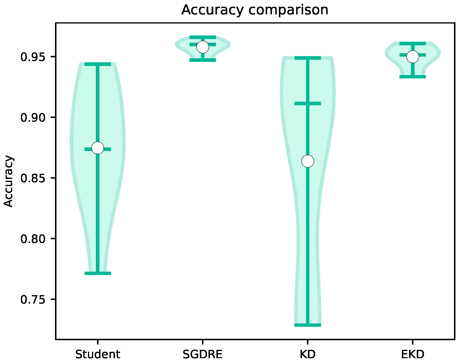
In Figure 7, the achieved accuracy values of the compared methods are presented in the form of violin plots. The violin plot is a combination of a box plot and a density plot, providing a deeper understanding of the distribution of metric values across 10 folds. The width of the violin plot represents the density of values in a range, meaning the wider the plot, the more values are presented in that range. The horizontal lines in each of the violin plots from top to bottom represent the maximum, median, and minimum values, while the white circle denotes the mean value.

Looking at the accuracy comparison, the EKD method achieves a high value of 0.95 with a standard deviation of 0.01, almost on par with the SGDRE method, which achieved 0.96. The difference between those two is only 0.01 on average. However, both of the mentioned methods outperformed the KD model by a large amount, 0.09 and 0.10, respectively, as well as the Student model. Looking at the standard deviations, we can also observe that SGDRE and EKD methods have drastically smaller standard deviations in comparison to the KD and Student models.

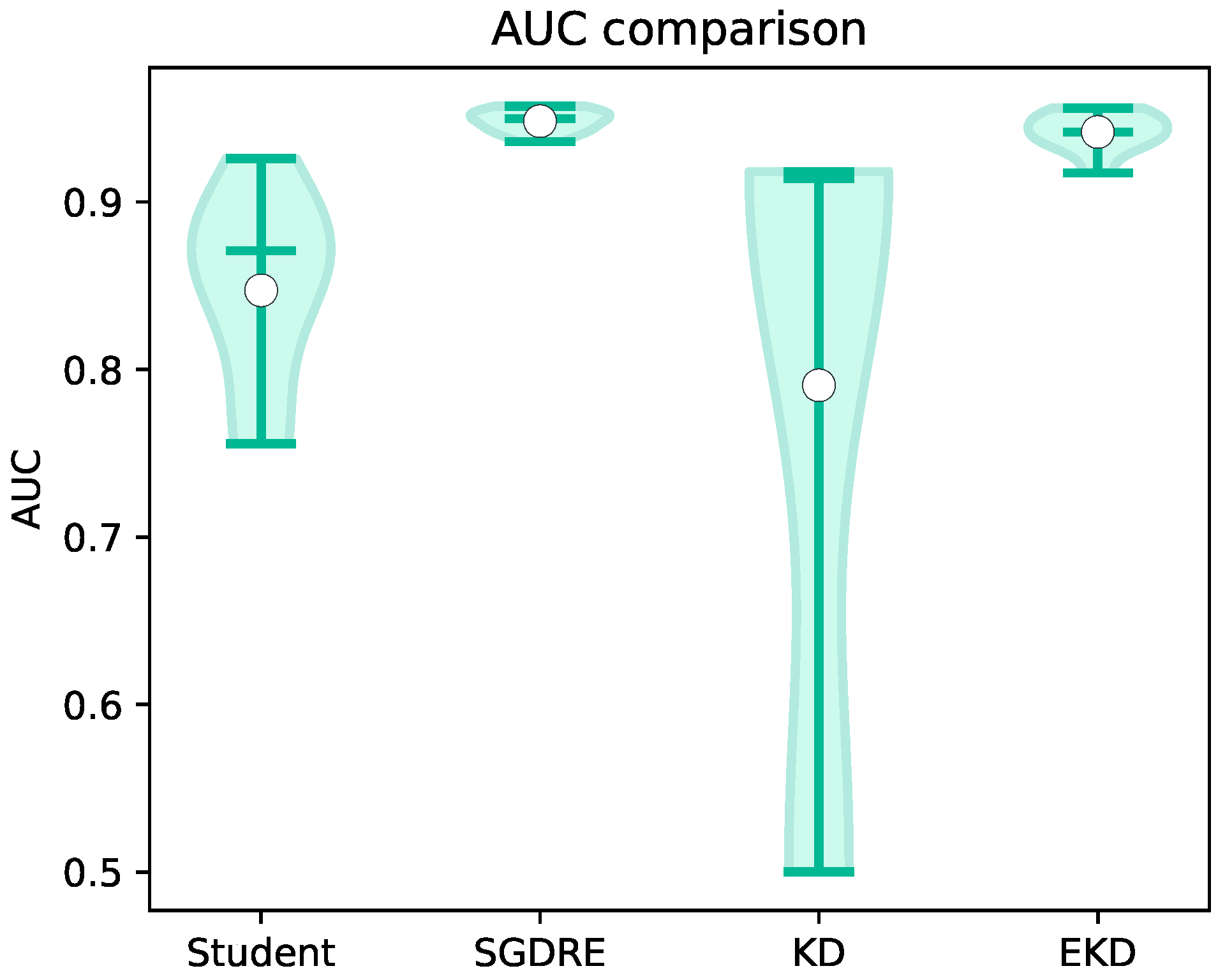
As is the case with the accuracy, we can also observe a similar pattern when comparing the AUC values presented in Figure 8. The delta between the best and second-best performing methods, namely SGDRE and EKD method, is at 0.01, while the delta between SGDRE and the worst-performing KD model is 0.16. Similar to the accuracy values distribution, we can also observe that the density of AUC values for the SGDRE and EKD methods is not as scattered as it can be observed with the KD and Student. Additionally, the KD model achieved by far the lowest AUC value, while the maximum value is similar to the worst performing fold of EKD model.

Focusing on the F1 values presented in Figure 9, we can see that the distribution of values across all methods is practically the same as was in the case of the AUC metric. The only difference is in the delta between the worst performing KD model and the best performing SDGRE model, which is in the case of the F1 metric set at 0.13.

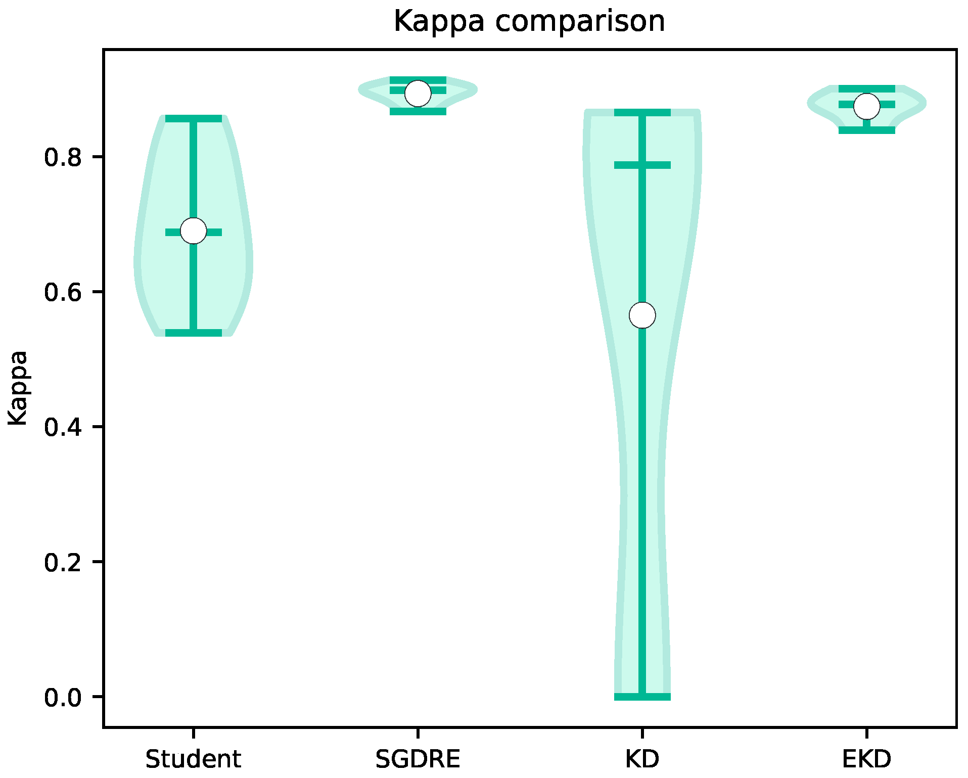
Figure 10 depicts the violin plots of kappa statistic values over 10 folds. In terms of achieved average kappa values, the best performing method is again the SGDRE method, achieving 0.89, followed closely by EKD method with 0.87, while the Student and KD models achieved 0.69 and 0.57, respectively. Looking at the delta values when comparing the SGDRE and EKD methods, we can observe a difference of 0.02. On the other hand, when comparing the SGDRE method against the KD model, the difference is 0.32. Interpreting the kappa statistic, based on the definition proposed by Landis and Koch [44], the SGDRE and EKD methods on average achieved almost perfect agreement, the Student model achieved substantial agreement, while the KD model achieved moderate agreement.

5.2. Computational Complexity Comparison

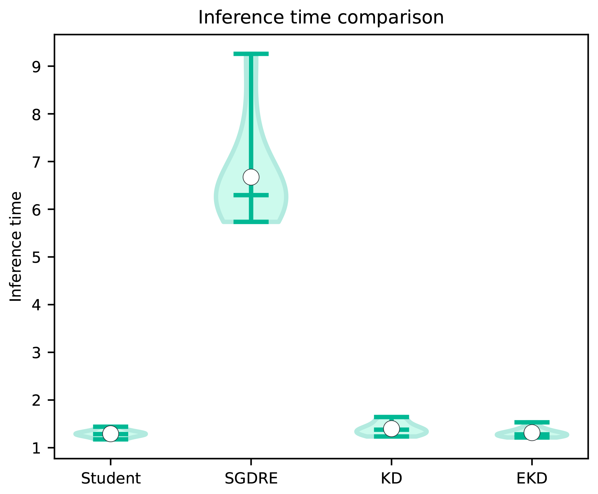
Figure 11 depicts the distribution of achieved inference times of the compared methods over 10 folds. These times are indicative of the computational complexity of each method during the inference. It must be noted that the inference time of a fixed architecture is inherently constant under deterministic conditions; any observed fluctuations are due to measurement noise introduced by interpreter-level overhead (e.g., from Python 3.11.3) or background operating system processes. Therefore, the observed minor differences in inference time between EKD, KD, and Student models are practically insignificant. As observed in the figure, the SGDRE method is by far the worst performing, trailing behind the second best EKD method by 5.36 s. It would be expected that the SGDRE method would take three times more inference time than the EKD, Student, or KD methods. However, in the case of the SGDRE method, we must also take into consideration the fact that there is some overhead when combining the predictions of each ensemble model. The distribution of the inference times of the SGDRE method is much more scattered than in the case of the compared methods. Such long inference times can be attributed to the fact that the SGDRE method needs to perform three predictions for each given test sample in order to compute the final prediction. When comparing the two best-performing methods, we can observe that the inference times are practically the same, with an average difference of 0.2 s.

In addition to the measured inference time, we also conducted a comparison between the SGDRE and the proposed EKD method. In

Table 3. Comparison of SGDRE method and Student/EKD model trainable parameters and FLOPs.

Metric	SGDRE	Student/EKD 1	Reduction Ratio
Parameters	20,386,182	4,737,698	4.31×
FLOPs	2,486,904,420	382,573,292	6.5×

¹ Student and EKD method have the same CNN architecture.

, the number of trainable parameters of the compared methods are presented together with the required FLOPs. As we can observe, the EKD method has a clear advantage also in that aspect due to the reduced size of the student CNN architecture. In terms of the reduction ratio, the number of trainable parameters was reduced by 4.31 times, while the FLOPs were reduced by 6.5 times.

5.3. Statistical Analysis

In order to assess the statistical significance of the obtained results, we followed the procedure suggested by Demšar [40]. First, we conducted a Shapiro–Wilk test to determine whether the values of each metric are normally distributed. Since the hypothesis was rejected, meaning the values are not normally distributed, we employed the Friedman test as suggested by calculating the asymptotic significance for all compared methods on all 10 folds. The results of the conducted test are presented in

Table 4. Statistical results of Friedman test.

	Friedman Test	Rank Averages 1
Metric	All Three	Student	SGDRE	KD	EKD
Accuracy	<0.001	3.60	1.15	3.3	1.95
AUC	<0.001	3.70	1.40	3.3	1.60
F1	<0.001	3.60	1.20	3.30	1.90
Kappa	<0.001	3.70	1.20	3.20	1.90
Time	<0.001	1.00	3.60	2.30	3.10
Epochs	<0.001	1.60	4.00	2.00	2.40

¹ Lowest average rank at the specific metric represents the better performing method. Bold values represent the best achieved score.

together with the rank averages for each method and metric.

Observing the results of the conducted Friedman test, we can see that there are statistically significant ($p<0.001$) differences between methods regardless of the metric. Therefore, we continue with the post hoc statistical analysis, conducting the Wilcoxon signed-rank test, which can be used to compare the statistical equality of two methods over the same sample. Since there were multiple comparisons between the methods, we applied the Holm–Bonferroni correction, which is used to control the family-wise error rate when conducting multiple hypothesis tests. The results of the conducted signed-rank test are presented in

Table 5. Results of Wilcoxon test with Holm–Bonferroni correction applied.

Metric	Student vs. SGDRE	Student vs. EKD	KD vs. EKD	SGDRE vs. EKD
Accuracy	0.047	0.047	0.047	0.297
AUC	0.047	0.047	0.047	0.422
F1	0.047	0.047	0.047	0.297
Kappa	0.047	0.047	0.047	0.297
Time	0.047	0.047	0.420	0.422
Epochs	0.047	0.422	0.422	0.047

Bold values represent the best achieved score.

. The table presents the pairwise comparison of models’ predictive performance methods for each metric. The emphasized values in the table represent the statistically significant differences, with a significance level of 95%. Focusing on the comparison between the Student and SGDRE, we can observe that there is a statistically significant difference between the compared methods for all metrics. Combining the results with the achieved rank averages presented in Table 4, we can observe that for the metrics accuracy, AUC, F1, and kappa, the SGDRE achieved a lower average rank, so it is considered better performing. However, for the metrics, time, epochs, and inference time, it is the other way around. Comparing the Student model with the EKD method, we can observe that there is a statistically significant difference for metrics accuracy, AUC, F1, Kappa, and training time. Looking at the average ranks, we can see that the proposed EKD method achieved statistically significantly better results for all the predictive metrics, and the Student model achieved statistically significantly lower training time. Those findings support the decision to utilize the proposed EKD method instead of training the Student network in a conventional manner (i.e., without knowledge distillation). If the EKD method does not yield a statistically significant performance improvement, the Student architecture would be a more reasonable choice in terms of training time.

When comparing the two knowledge distillation approaches, KD and EKD, we observe a statistically significant difference in the metrics of accuracy, AUC, F1, and Kappa. Inspecting the average ranks, we can see that the proposed EKD method achieves statistically significantly better results across all predictive metrics. In contrast, differences in training and inference times are statistically insignificant, as expected, since both approaches use the same student architecture.

Finally, comparing the best performing SGDRE method with the proposed EKD method, we can see that the statistically significant differences are only present for the metrics epochs and inference time. The predictive performance metrics and training time are not statistically significantly different; therefore, we can confirm that the predicting performance of the proposed EKD method is comparable to the more computationally complex SGDRE method. Focusing on the metrics epochs and inference time, looking at the average ranks achieved, we can see that the EKD method achieved, on average, lower ranks than the SGDRE method. Thus, the proposed method is statistically significantly better performing in terms of epochs needed to train and, more importantly, achieves faster inference time, due to reduced computational complexity.

5.4. Comparison with Some Existing Methods

Several studies have used the same chest X-ray dataset to detect childhood pneumonia. However, it is important to note that not every study employed the same evaluation methodology (using k-fold cross-validation versus using simple train test split approach). As a result the comparison may not be entirely objective, but it can still provide a general sense of the predictive performance landscape across different approaches.

Kermany et al. [39] presented a method which utilizes the transfer learning approach using the Inception V3 CNN architecture. The authors reported an accuracy of 92.8%, which lags behind the proposed EKD method by 3.2%.

A study conducted by Stephen et al. [37] proposed a specific custom CNN architecture that achieved an accuracy of 93.7%. In comparison, the proposed EKD method outperforms this by a margin of 2.3%.

In [28], Asham et al. presented a lightweight deep learning model with KD, which achieved an accuracy of 97.92%, exceeding that of the EKD method by 1.92%. However, the experiments conducted by Asham et al. employed a simple train/validation/test split methodology, which could have contributed to the reported predictive performance difference.

Kundu et al. [49] reported that their proposed ensemble method achieved an average accuracy of 98.81% and an average F1 score of 98.97, surpassing the EKD method by 2.81 and 3.79, respectively. While it is not uncommon for ensemble methods to outperform single-model methods on specific tasks, they pose challenges for deployment in resource-constrained environments due to increased computational complexity during inference.

Singh et al. [19] proposed an efficient detection method based on Vision Transformers. The authors conducted extensive performance evaluation relative to other architectures utilizing the same dataset. Their proposed Vision Transformer method achieved an accuracy of 97.61% and an F1 score of 0.95. Compared to the EKD method, this represents a 1.61% higher accuracy, while on average achieving the same F1 score. Additionally, from the computational complexity standpoint, we can also observe that proposed EKD method has around 17 times fewer trainable parameters than the Vision Transformers method, which translates to significantly shorter training and inference time.

6. Discussion

Following an in-depth analysis of the experimental results, we confirm that the model trained using our proposed EKD method achieved predictive performance comparable to that of the more computationally complex SGDRE method when applied to the task of identifying childhood pneumonia from X-ray images. The predictive metrics were statistically insignificantly different from the SGDRE method, while the inference time was significantly different. Observing the average ranks proved that the proposed EKD achieved on average a lower rank; therefore, it is better performing in terms of inference time. Additionally, the computational complexity of the proposed EKD method in comparison to the SGDRE method was reduced by a factor of 6.5× in terms of FLOPs standpoint and 4.31× in terms of the number of trainable parameters.

When comparing the predictive performance of the EKD model with that of the Student and KD methods, we observed that the EKD model significantly outperformed both in all classification metrics by a great margin. These findings support the utilization of the proposed EKD method instead of utilizing the Student CNN architecture and training it in a conventional manner. However, the training time of the Student method was significantly better than that achieved by the EKD method. We can attribute this to the fact that in the process of knowledge distillation, for each iteration of training, it is needed to obtain the prediction of teacher models in order to compute the soft labels. Therefore, the training time is increased in comparison to the conventional training of CNN.

Based on the obtained empirical results, we can confirm that the proposed EKD method can match the predictive performance of the more complex SGDRE method in the task of childhood pneumonia identification, while simultaneously reducing both computational complexity and inference time.

Although the reported performance remains strong, a limitation of the current study is the absence of explicit strategies to address class imbalance in the training data. Future work will explore the use of data augmentation, re-sampling, and class weighting techniques to further enhance model fairness and ensure more robust detection of underrepresented classes.

7. Conclusions

In this study, we proposed an ensemble-based knowledge distillation method for classification problems and applied it to the task of identifying childhood pneumonia from X-ray images. The method utilizes the SGDRE approach for the purpose of obtaining a homogeneous group of specialized CNN models, which are utilized as a group of teacher models. From the obtained group of models, the top three most suitable models are selected as the teacher models in the process of distilling the knowledge to a smaller, more efficient student CNN model.

The model trained using the proposed method was empirically evaluated on the task of childhood pneumonia identification and compared with both the SGDRE ensemble method and the Student CNN architecture trained using a conventional approach. Statistical analysis of the obtained results demonstrated that the proposed EKD method significantly outperformed the conventionally trained Student model and achieved comparable performance to the more computationally complex SGDRE method, while providing statistically significantly faster inference times.

In future work, we would like to expand our work to explore the possibility of implementing fully automatic, adaptive computation of the distillation loss throughout the knowledge distillation process, with the goal of further improving the predictive performance of the proposed method.