Abstract
Recent advancements in implicit neural representations have shown substantial promise in various domains, particularly in video compression and reconstruction, due to their rapid decoding speed and high adaptability. Building upon the state-of-the-art Neural Representations for Videos, the Expedite Neural Representation for Videos and Hybrid Neural Representation for Videos primarily enhance performance by optimizing and expanding the embedded input of the Neural Representations for Videos network. However, the core module in Neural Representations for Videos network, responsible for video reconstruction, has garnered comparatively less attention. This paper introduces a novel High-frequency Spectrum Hybrid Network, which leverages high-frequency information from the frequency domain to generate detailed image reconstructions. The central component of this approach is the High-frequency Spectrum Hybrid Network block, an innovative extension of the module in Neural Representations for Videos network, which integrates the High-frequency Spectrum Convolution Module into the original framework. The high-frequency spectrum convolution module emphasizes the extraction of high-frequency features through a frequency domain attention mechanism, significantly enhancing both performance and the recovery of local details in video images. As an enhanced module in the Neural Representations for Videos network, it demonstrates exceptional adaptability and versatility, enabling seamless integration into a wide range of existing Neural Representations for Videos network architectures without requiring substantial modifications to achieve improved results. In addition, this work introduces the High-frequency Spectrum loss function and the Multi-scale Feature Reuse Path to further mitigate the issue of blurriness caused by the loss of high-frequency details during image generation. Experimental evaluations confirm that the proposed High-frequency Spectrum Hybrid Network surpasses the performance of the Neural Representations for Videos, the Expedite Neural Representation for Videos, and the Hybrid Neural Representation for Videos, achieving improvements of +5.75 dB, +4.53 dB, and +1.05 dB in peak signal-to-noise ratio, respectively.
1. Introduction
Global internet traffic has been experiencing a steady growth rate of approximately 22% annually, currently surpassing 33 exabytes per day [1]. This rapid increase is largely driven by the rising demand for high-definition video across various applications, such as video conferencing, security surveillance, medical care, agriculture, forestry, and online video streaming platforms like YouTube and Netflix. Despite advancements in hardware storage and network transmission technologies, the sheer size of uncompressed raw video files continues to pose significant challenges in terms of storage capacity and bandwidth requirements. As a result, video compression has emerged as a critical area of research, focused on developing methods that reduce the volume of video data while preserving as much visual quality as possible after reconstruction.
Traditionally, video encoding has relied on techniques such as the discrete cosine transform (DCT) [2] and predictive coding across spatial and temporal domains. However, deep learning-based video compression algorithms offer considerable advantages, particularly in terms of end-to-end optimization, improved quality retention, and enhanced compression ratios. Prominent works in this domain include learning-based modules for adapting conventional codecs [3,4,5,6,7,8] and end-to-end video compression models [9,10,11,12,13,14,15,16]. Moreover, Neural Representations for Video (NeRV), models [17,18,19,20], which are based on implicit neural representations, have garnered widespread attention due to their simplicity, high adaptability, and exceptionally fast decoding speeds. Notable recent advancements include the Expedite Neural Representation for Videos (E-NeRV) [18] and Hybrid Neural Representation for Videos (HNeRV) [19], which offer significant improvements in the efficient reconstruction of video frames with superior quality compared to the original NeRV model [17].
Although E-NeRV [18] and HNeRV [19] have achieved promising results, research on NeRV still faces several limitations and challenges.
Firstly, while both E-NeRV [18] and HNeRV [19] achieve marginal improvements by adjusting the number of channels in NeRV blocks, their superior performance primarily arises from the optimization of the input embeddings in the NeRV network. In [17], Chen et al. used frame indices, which are simple scalar values, as temporal input embeddings. E-NeRV [18] further enhanced this approach by incorporating spatial coordinates as spatial embeddings. HNeRV [19] enriches the spatial embeddings by extracting feature maps from the ground-truth video images, employing ConvNeXt [21] (a regular Convolutional Neural Network (CNN)) as an encoder. While improving the quality of input embeddings is a highly effective strategy for enhancing model performance, increasing the efficiency of the NeRV block itself remains a critical concern.
Secondly, the current best-performing model, HNeRV [19], exhibits limitations in generating visually coherent images, leading to the loss of texture and edges. Figure 1 provides an illustrative example. HNeRV [19] fails to capture the edge details of the nose and mouth when reconstructing a character’s face, and introduces noise points that affect color uniformity across the face. We hypothesize that the narrow receptive field and absence of high-frequency information are the primary causes of this phenomenon. First, small convolutional kernels are limited in the range of features they can capture, which can lead to incorrect pixel values being generated by the network. Although increasing kernel size effectively expands the receptive field and improves performance, it also results in a significant increase in network parameters, which grows quadratically. Second, convolution is a weighted summation operation that tends to produce smooth, low-frequency information over broad regions rather than high-frequency signals with sharp local variations. This limitation hinders the network’s ability to accurately reconstruct object edges and texture details. Although high-frequency details may be prioritized under a constrained compression ratio, the human visual system remains highly sensitive to such details, such as textures and edges. Loss of these elements causes videos to appear blurred, which is especially noticeable in scenes requiring fine detail, such as satellite imagery, medical videos, and game streaming.
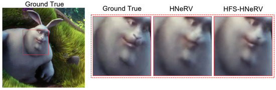
Figure 1.
An example of missing texture and edges.
In light of these challenges, our research is motivated by the following considerations:
- Existing NeRV-type methods primarily focus on incorporating multimodal or enhanced input data to improve video reconstruction, rather than enhancing the intrinsic performance of the network modules themselves. Although modifying the input data is less likely to introduce fluctuations in model parameters to affect the compression rate, it remains essential to design a new core module to enhance the intrinsic performance of the network.
- Although current NeRV-type approaches can learn implicit representations of video frames, they lack dedicated modeling of high-frequency information, resulting in insufficient detail reconstruction. Therefore, a novel fundamental module capable of reconstructing high-frequency content is required.
Based on the aforementioned motivations, we propose an innovative approach called High-frequency Spectrum Hybrid Neural Representation for Video (HFS-HNeRV). Figure 2 illustrates the primary architecture and workflow of HFS-HNeRV. To address the first challenge, we introduce the HFS-HNeRV block, which enhances the basic NeRV module by incorporating a high-frequency spectrum convolution module (HFSCM). HFSCM includes a high-spectral attention mechanism based on the channel–spatial attention structure of CBAM [22] and GAM [23], along with an additional convolutional layer. Channel attention reweights each channel in the feature map by integrating the information of all channels for each pixel, encouraging the model to focus on channels that are most critical to overall semantics. Spatial attention allows the model to highlight regions that are vital to global semantics along the spatial dimension. Moreover, since the channel dimension can be greatly reduced in spatial attention, a larger receptive field (such as a large convolution kernel) can be applied without substantially increasing the number of parameters. This design allows the model to integrate a wider range of local contextual information with only a minimal increase in parameter count, thereby considering more global semantic information when redistributing weights. After the attention module accentuates the important feature information, the subsequent convolutional layers not only expand the receptive field but also further fuse these attention-weighted features to generate richer and higher-quality feature representations. This modification significantly improves video frame reconstruction while maintaining a stable parameter count. The HFS-HNeRV block also exhibits excellent compatibility and generalizability, making it easily integrable into a wide range of NeRV networks without necessitating significant changes to the original architecture.
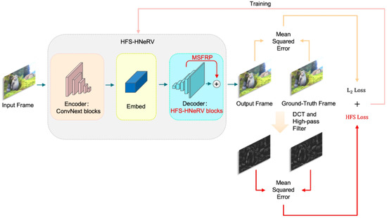
Figure 2.
Our proposed HFS-HNeRV enables the model to focus on the details of edges and textures in the image by introducing the HFS attention mechanism, HFS loss, and multi-scale feature reuse.
To address the second challenge, the proposed HFSCM includes a novel high-frequency enhancement attention mechanism, which leverages the Haar wavelet transform to strengthen high-frequency components. This technique effectively captures the high-frequency features within the feature map, facilitating the restoration of edge details and textures, thereby enhancing the overall image quality. Additionally, the attention mechanism enables the module to better extract and fuse global information, partially mitigating the issue of insufficient receptive fields. Furthermore, HFSCM incorporates a dual convolutional layer structure, which further refines the features enhanced by the high-frequency spectrum attention mechanism (HFSAM), resulting in richer feature representations.
We also propose a high-frequency spectrum loss function to aid in the training of the model. This loss function extracts high-frequency signals from both the predicted and ground-truth images via Fourier transform and high-pass filters and then computes the mean square error (MSE) between them. The high-frequency spectrum (HFS) loss is integrated into the overall loss function alongside the MSE loss, with a hyperparameter introduced to adjust its weight relative to the total error. This adjustment allows the model to reduce the disproportionate influence of low-frequency components, thereby encouraging greater focus on generating finer image details, such as edges and textures.
Finally, inspired by classical image and video super-resolution networks, we introduce several modifications to the decoder’s structure. Specifically, we incorporate a multi-scale feature reuse path (MSFRP), which enriches the final output feature representations by fusing feature maps from different scale layers.
In summary, our work makes the following contributions:
- We propose a novel NeRV module, HFS-HNeRV block, which can be easily integrated into various NeRV networks without substantial modifications to the network architecture.
- We introduce a new loss function specifically designed for high-frequency information generation, enhancing the model’s capacity to reconstruct image details.
- We optimize the NeRV network design by incorporating MSFRP into the current NeRV framework.
2. Related Works
2.1. Implicit Neural Representations
Implicit neural representations [24], often applied in image [25,26] or scene reconstruction [27,28], are techniques that utilize neural networks to represent geometric shapes or environments. For example, Neural Radiance Fields (NeRFs) [28] can reconstruct a 3D scene using provided 3D coordinates. In NeRV [17], the entire video or image sequence is implicitly represented by a neural network instead of being stored in the traditional form of frame data. The network learns the mapping from input (such as timestamps or spatial coordinates) to output (image frames) so that it can quickly decode the video frames based on frame indices. Unlike explicit representations, implicit representations store most of the information in the network’s parameters, which significantly reduces storage requirements. However, implicit representations come with several drawbacks. They demand substantial resources during the training process—such as extensive training time, large datasets, and significant computational power—which makes their application in real-time scenarios challenging. Additionally, the complexity of these models can lead to instability during training.
2.2. Video Compression
Video compression seeks to reduce the size of video data while preserving as much quality as possible. Conventional video compression standards, such as H.264 [29] and H.265 [30], have been widely used across many fields. In the past decade, deep learning has introduced new possibilities for advancements in video compression techniques. Traditional methods typically involve four core technologies: predictive coding, transform coding, entropy coding, and motion compensation. Learning-based video compression approaches primarily focus on replacing or enhancing these key components [3,4,5,6,7,8]. Additionally, Refs. [9,10,11,12,13] have explored end-to-end video compression models. However, a novel approach called Neural Representations for Videos (NeRV) [17] has been introduced, which uses neural networks to implicitly represent video by overfitting the network to memorize video frames. By compressing the neural network, NeRV achieves the goal of video compression.
2.3. Video Super-Resolution
Video super-resolution is a technique widely applied in fields such as remote sensing and telemedicine to enhance both the resolution and visual clarity of video frames. At its core, it primarily involves upsampling methods, including interpolation, pixel shuffle, and deconvolution. The deep learning-based approaches to video super-resolution can be broadly classified into single-frame [31,32,33,34,35] and multi-frame methods [36,37,38,39,40,41]. Given that video is essentially a sequence of consecutive images forming a dynamic visual record, single-frame super-resolution networks are largely extensions of image super-resolution techniques. Prominent examples include the Super-Resolution Convolutional Neural Network (SRCNN) [31], Very Deep Super-Resolution (VDSR) [32], and the Super-Resolution Generative Adversarial Network (SRGAN) [35]. In contrast, multi-frame super-resolution networks exploit the inter-frame information present in videos, and these methods can be further subdivided into those that align video frames and unaligned methods. Approaches based on optical flow estimation [38,39] and deformable convolution [40,41] are key examples of the former, whereas those employing 3D convolution [42,43] and recurrent convolutional neural networks [44,45] exemplify the latter. The primary objective of video super-resolution is to upsample low-resolution videos into high-resolution counterparts. This procedure bears similarities to how NeRV [17] incrementally upsamples an embedding into a complete video image, thus creating some overlap in the methodologies used in these two areas. Low-quality videos can be considered compressed versions of their high-resolution counterparts. NeRV-like approaches may draw inspiration from video super-resolution techniques, such as more sophisticated network designs (encoder–decoder model and Generative Adversarial Network (GAN) [46]) and enhanced upsampling mechanisms (such as bilinear interpolation and Sub-pixel Convolution). Nevertheless, since the parameter count in NeRV models directly influences the compression ratio, any method that substantially increases model complexity should be applied judiciously. For more detailed comparisons of video super-resolution models, please refer to [47,48,49].
2.4. Frequency Domain Image Analysis
Although images have traditionally been processed in the spatial domain for computer vision tasks, recent studies [50,51] have demonstrated that frequency domain analysis offers distinct advantages, particularly in image compression. The HFSAM proposed in this study differs from these prior works in several key aspects.
The core concept of LC-FDNet [50] is adaptive frequency decomposition (AFD), which extracts low-frequency (LF) and high-frequency (HF) latents from input images, followed by separate compression. Specifically, the high frequency compressor retains the residual information between the original image and the high-frequency prediction generated by the network, leveraging entropy coding for compression. The principal objective of this approach is to extract and compress the low- and high-frequency components separately, thereby mitigating information loss during the compression process.
DBPN [51] separates the low- and high-frequency latents by using average pooling. These latents are subsequently processed through a dual-layer attention mechanism to generate an attention map. In the process of obtaining the final output latent, they recall the low frequency and high frequency latents to emphasize these fine-grained features again. In our approach, we integrate the Haar wavelet transform into the spatial attention component to extract high-frequency information, further weighting the LH, HL, and HH components using hyperparameters. This weighting strategy ensures that these high-frequency details receive emphasis in the generated attention map.
Similarly, the Frequency-Aware Transformer [52] introduces the frequency-decomposed window attention (FDWA) mechanism to achieve frequency decomposition, grounded in the theoretical foundation that small local window attention can effectively capture high-frequency information, as discussed by [53]. This effect closely resembles that of the Haar wavelet transform, which also produces the LL, LH, HL and HH maps. Fundamentally, both methods serve to decompose images into their low- and high-frequency components. Structurally, FDWA integrates self-attention with window attention, making it particularly well suited for transformer architectures. In contrast, Convolutional Neural Networks (CNNs) can achieve a similar effect more efficiently by directly applying the Haar wavelet transform for frequency decomposition and integrating spatial and channel attention mechanisms to enhance the representation of edges and texture details.
3. Proposed Method
Figure 3a,b show the overall structure of the HFS-HNeRV network. In Section 3.1, we will explain the structure and function of the key parts in the HFS-HNeRV block. Section 3.2 is an introduction to MSFRP. Finally, the HFS loss function is described in Section 3.3.
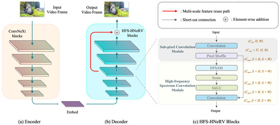
Figure 3.
The structure of HFS-HNeRV. (a) Encoder: we employ ConvNeXt as the encoder to downsample the input video frames into smaller embeddings. (b) Decoder: we employ the HFS-HNeRV blocks to build the decoder for upsampled images and add MSFRP to reuse the feature maps of the third layer. (c) HFS-HNeRV blocks: In the HFS-HNeRV blocks, we introduce a residual structure that, through dual convolutional layers, further enriches the generated features by leveraging the attention maps produced by HFSAM.
3.1. HFS-HNeRV Block
As can be seen in Figure 3c, HFS-HNeRV block is composed of a sub-pixel convolution module and HFSCM.
3.1.1. Sub-Pixel Convolution Module
For the first half of the HFS-HNeRV block, we retain the sub-pixel convolution (SPC) module. It has been employed as a basic module in previous NeRV-type works. Detailed information can be found in [33]. Here, we only give a brief introduction.
The SPC module integrates a convolutional layer with a pixel shuffle layer. In the convolutional process, as shown in Figure 3c, the input feature map adheres to the dimensions , while the output feature map is represented as . This dimensionality enhancement can be interpreted as the network layer extracting features, which subsequently serve as references for generating more contextually relevant features. A reduction in the number of input or output channels will significantly degrade the performance of this network layer. Although increasing the size of the convolutional kernel can improve network efficiency, it also results in a considerable increase in the number of model parameters. Therefore, to ensure parameter stability, the original kernel size and channel configuration have been maintained.
3.1.2. High-Frequency Spectrum Convolution Module
HFSCM is primarily composed of two components: a high-frequency spectrum attention mechanism and an additional convolutional layer. As depicted in Figure 3c, the entire module adopts a residual block structure.
The high-frequency spectrum attention mechanism (HFSAM) consists of two key parts: the channel attention layer and the frequency domain spatial attention layer. The channel attention layer employs a dual multi-layer perceptron structure to produce a channel attention map by extracting global information from the feature vectors at each position within the feature map , as demonstrated in Figure 4a. This process can be expressed by the following formula:
where denotes the sigmoid function. represents the GeLU activation function. ⊗ represents the element-wise multiplication. represents the multi-layer perceptron. represents a convolutional layer.
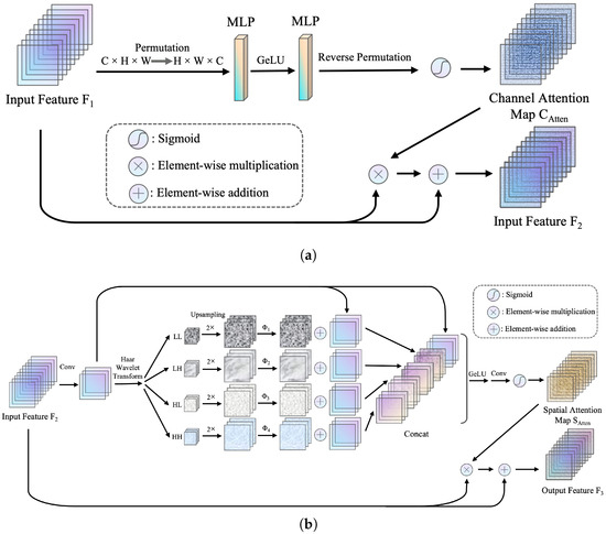
Figure 4.
(a) Channel Attention: This part employs dual multi-layer perceptron to integrate the intra-channel contextual information of the input features, computing the output feature map through a residual structure. (b) Spatial Attention: We enhance high-frequency information by incorporating Haar wavelet transform into the spatial attention mechanism. Note that symbolizes the two-fold upsampling operation.
Before introducing the frequency domain spatial attention layer, we briefly describe the processing of the Haar wavelet transform on the feature map. The Haar wavelet basis functions are defined by the scaling function and the wavelet function :
For a one-dimensional signal x of length N, the corresponding low- and high-frequency operators are denoted and , respectively:
where .
Since the Haar wavelet transform is applied to the feature map on a channel-by-channel basis, only a two-dimensional Haar wavelet transform is required. First, the operator transforms each row of the feature map to obtain a new matrix :
Next, the columns of are transformed to yield the matrix :
Finally, the matrix is partitioned into four sub-regions:
where denotes the low–low subband, representing the approximation coefficients after applying low-pass filtering in both horizontal and vertical directions. represents the low–high subband, containing vertical detail coefficients obtained by low-pass filtering horizontally and high-pass filtering vertically. represents the high–low subband, containing horizontal detail coefficients obtained by high-pass filtering horizontally and low-pass filtering vertically. denotes the high–high subband, capturing diagonal detail coefficients after applying high-pass filtering in both horizontal and vertical directions. More detailed information about the Haar wavelet transform can be found in [54].
In the frequency domain spatial attention layer, as depicted in Figure 4b, the initial convolutional layer is designed to reduce the number of channels in the input feature map . This reduction primarily aims to minimize the number of parameters in the attention layer, ensuring computational efficiency. Following this, the feature map undergoes decomposition into various frequency component sub-maps through the Haar wavelet transform, producing the low frequency–low frequency (LL) map, low frequency–high frequency (LH) map, high frequency–low frequency (HL) map, and high frequency–high frequency (HH) map. After decomposition, the sub-maps are upsampled to match the original feature map’s dimensions. Each of these four sub-maps is then multiplied by a set of distinct enhancement weights, followed by element-wise addition with the original input feature map. These four enhanced sub-maps are concatenated with the input feature map, forming an enriched feature representation. The concatenated feature map is subsequently processed through a sequence of layers, including normalization, activation, convolution, and sigmoid functions, resulting in the generation of the spatial attention map . The incorporation of the Haar wavelet transform enables the analysis of frequency domain information, allowing the HFSCM to capture high-frequency features more effectively. This leads to the restoration of edge details and textures within the image, thereby improving the overall quality of image generation. Additionally, the use of the attention mechanism strengthens the module’s ability to extract and integrate global information, partially alleviating the issue of insufficient receptive field. The calculation process for spatial attention is described as follows:
where denotes the bilinear interpolation operation, and represents the Haar wavelet transform. represents the enhancement factor of the frequency maps. , , , and represent the feature maps for the , , and sub-bands, respectively. represents the concatenation operation that merges multiple tensors.
In addition, we introduced extra convolutional layers following the HFSAM (as shown in Figure 3c) to allow the network to better focus on and exploit the high-frequency features enhanced by the HFSAM. The additional convolutional layers expand the receptive field, thereby enhancing the model’s ability to represent intricate high-frequency details. The shortcut connection contributes to the overall stability of the module during training to avoid the problem of gradient disappearance. The following formula can be used to express how the feature map is calculated:
where ⊕ denotes the element-wise addition.
3.2. Multi-Scale Feature Reuse Path
MSFRP, whose structure is shown in Figure 5, enables the model to capture more information at different scales and further enhances the model’s expressiveness. In the NeRV-based network, avoiding growth of the number of parameters is an essential prerequisite. Therefore, we decide to upsample the feature map produced by the model’s third-to-last layer via the bilinear interpolation method to the same size as the final output feature map of the model. Specifically, the feature maps from layers are first reduced to the channels at 3 through a convolutional layer. Then, they are resized to a common spatial resolution via bilinear interpolation. Finally, the aligned feature maps are fused by element-wise addition. Bilinear interpolation is a technique that involves two linear interpolations in a two-dimensional plane grid cell. Assuming that the coordinates of the four corners of the grid cell are , , and , the bilinear interpolation polynomial formula can be expressed as
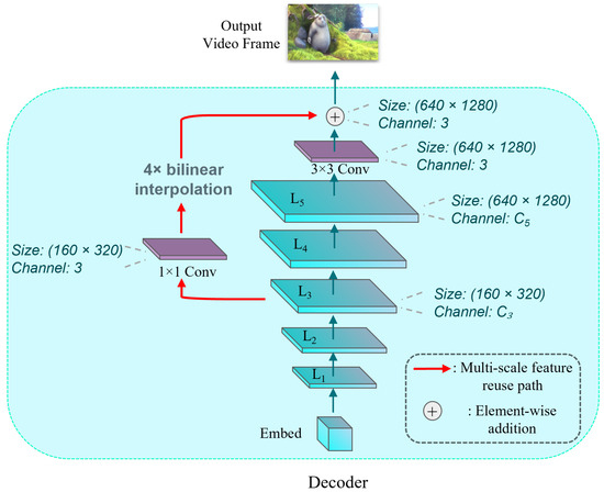
Figure 5.
The structure of MSFRP.
Detailed information on bilinear interpolation can be found in [55].
3.3. High-Frequency Spectrum Loss
The MSE loss function is widely used in various downstream tasks within computer vision. To further direct the model’s focus towards high-frequency features in images, we introduce the HFS loss, which is based on the Fourier transform and high-pass filters, and incorporate it into the total loss function.
Specifically, we first transform both the predicted and ground-truth images into the frequency domain by employing the 2D discrete Fourier transform (DFT), implemented via PyTorch’s torch.fft.fft2. The zero-frequency component is shifted to the center of the spectrum to facilitate the application of a high-pass filter.
The high-pass filter is constructed as a binary circular mask that suppresses low-frequency components. Specifically, for a frequency spectrum of size , we set a square region of size , centered at , to zero. Here, m is a tunable cutoff parameter controlling the frequency threshold. The mask is broadcasted across batch and channel dimensions to match the shape of the input tensors.
After masking, we apply an amplification factor g to the remaining high-frequency components to emphasize fine-grained details such as edges and textures. Then, the filtered and enhanced frequency spectra are transformed back to the spatial domain by using the inverse 2D DFT. The HFS loss is defined as the mean square error between the spatial domain reconstructions derived from the high-frequency components of the predicted and ground-truth images.
The DFT and inverse DFT of a two-dimensional image can be represented as follows:
where H and W represent the height and width of the image, respectively. x and y denote the spatial coordinates within the image, and u and v represent frequency coordinates within the spectrum.
Given a video sequence and a frame index t, we have a predicted image and a ground-truth image . The formulae for MSE loss and HFS Loss are expressed as
where H and W represent the height and width of the image, respectively. C represents the number of channels of the image. and represent the predicted image and ground-truth image, respectively. , , M and g denote discrete Fourier transform, inverse discrete Fourier transform, binary high-pass filter mask, and high-frequency amplification factor, respectively.
The total loss function can be expressed as
where is the weight that controls the influence of HFS loss. It is set to 0.12 in the experiments.
4. Experiments
In this section, we will conduct ablation experiments on HFSCM, HFS loss, and MSFRP, and discuss their effectiveness in detail. We will initially go over the experimental setting and dataset that were employed in this study. Following Section 4.1, we will demonstrate the effectiveness of HFSCM, HFS loss, and MSFRP through ablation experiments in Section 4.2. Finally, Section 4.3 will show the performance of HFS-HNeRV in video compression tasks, including performance indicators and comparison of generated images.
4.1. Dataset and Implementation Details
In this paper, we utilize the hybrid representation network architecture of HNeRV. Therefore, most of the experimental settings are consistent with HNeRV. For the dataset, we adopt the Big Buck Bunny (the Big Buck Bunny dataset is available at https://github.com/haochen-rye/HNeRV (accessed on 25 June 2024)), a widely used open-source animated video, which includes 132 frames with resolution of , cropped to the center with a resolution of . The selected segments depict an animal coming out of a tree hole and stretching as it stands upright, covering a range of scenes with different levels of motion (from static to moving objects) and texture complexity (such as smooth backgrounds and detailed foliage or grass). To evaluate the model’s performance on a publicly available benchmark, we applied center cropping to the UVG dataset (the UVG dataset is available at https://ultravideo.fi/dataset.html (accessed on 28 December 2024)) (7 videos in full HD resolution () with a frame rate of 120 frames per second (fps)), resulting in a resolution of . They include fast motion (such as a speedboat, bee wings, and running horse), high-frequency textures (such as long hair, petals and waves), and rich structural information, making it suitable for evaluating the generalization and robustness of video reconstruction models. For performance metrics, we retained the same settings as those in HNeRV [19], specifically the peak-signal-to-noise ratio (PSNR) and multi-scale structural similarity index measure (MS-SSIM). Moreover, we selected multiple regions within the images to conduct a human visual quality comparison. During training, we used the Adam optimizer with and a weight decay of 0. Furthermore, we set the learning rate to 0.001 with cosine learning rate decay. Unless otherwise stated, all experimental models are baselined with model size of 1.5 M, training epochs of 300, and bit per pixel (bpp) of 0.109. All experiments were conducted on one laptop-based RTX 3060 GPU. the reported performance results were also measured on this GPU to reflect parallel execution, excluding data loading and preprocessing overhead.
4.2. Ablation Study
In this section, we will present and discuss the relevant ablation experiments of HFSCM, HFS loss, and MSFRP, and explain their related parameter settings.
4.2.1. HFSCM
As shown in Table 1, inserting the attention module after the upsampling layer can significantly enhance model’s performance. Furthermore, HFSCM only introduces few parameters since the number of channels is kept low after the upsampling layer. The convolution layer after the attention mechanism can further combine local and global information to enhance the expressive capability of the model. Also, the residual structure not only prevents the gradient vanishing problem but also contributes positively to the performance of the model. The attention mechanism involves the convolution kernel size k in spatial attention. As mentioned earlier, a larger convolution kernel size will have a positive impact on model performance (as shown in Table 2). However, increasing the number of convolution kernels directly results in a growth in model parameters. Therefore, we conducted ablation experiments under conditions where the number of parameters and bit rate were kept at comparable levels (as shown in Table 3), and we then selected as a trade-off between model complexity and performance. Table 4 shows that the additional convolutional layers indeed have a significant positive impact on the performance of the model.

Table 1.
Comparison of module ablation experimental results.
Table 2.
Ablation of kernel size k under unconstrained settings (with ).
Table 3.
Ablation of kernel size k under parameter and bitrate constraints (with ).
Table 4.
Ablation of additional convolutional layer in HFSCM.
4.2.2. MSFRP
As can be seen in Table 1, the performance of variant 2 proves the effectiveness of reusing features of different scales. Considering that deconvolution or pixel shuffle will bring additional parameter burden, we apply the bilinear interpolation method rather than sub-pixel convolution or deconvolution. We consider that the output features of the third-to-last layer not only retain rich original feature information but also have a moderate level of feature abstraction. Upon comparison, it is clear that reusing the features of the third-to-last output layer has the best effect (Table 5). Since reusing the first layer necessitates upsampling by a factor of up to 64×, and the fifth layer serves as the network’s final output, the results from these two layers are excluded from Table 5.
Table 5.
Ablation of reusing different feature layers.
4.2.3. HFS Loss
HFS loss extracts the high-frequency features of generated images and ground-truth images through Fourier transform and high-pass filters before calculating the error between them. Table 1 demonstrates that the application of HFS loss can significantly boost the performance of the model. Table 6 shows the performance parameters of the model at different training cycles and the convergence of HFS loss. We set the threshold m and enhancement factor g of the high-pass filter to and , respectively. The PSNR results are shown in Table 7 and Table 8. The optimal hyperparameter settings are found to be and .
Table 6.
HFS loss ablation at different epochs.
Table 7.
Threshold m ablation (with ).
Table 8.
Enhancement factor g ablation (with ).
4.3. Main Results
4.3.1. Video Regression
In comparison to existing methods, our approach demonstrates improvements in both model performance metrics and human visual perception. All experiments were conducted using the Big Buck Bunny dataset. As shown in Table 9, with a model size of 1.5 M, HFS-HNeRV outperforms NeRV, E-NeRV, and HNeRV across various training epochs. Furthermore, when the training epochs are set to 300, HFS-HNeRV continues to deliver superior performance with 1.5 M parameters (Table 10). Table 11 shows that HFS-HNeRV can still maintain its performance advantage over HNeRV on the UVG dataset. Significantly, NeRV-based methods perform well on HoneyBee but show relatively poor performance on Ready and Yacht. This phenomenon can be analyzed from two main aspects: content complexity and motion intensity. First, regarding content complexity, the main subject in HoneyBee is a bee, which occupies only a small region in the entire frame. The background primarily consists of flowers and grass with simple structures and similar color distributions. This implies that the model needs to learn fewer and less complex visual features. In contrast, Yacht and Ready contain abundant high-frequency details (such as water ripples, human contours, and hair), which place higher demands on the model’s representational capacity. Although our method achieves notable improvements over HNeRV on these videos, the overall performance remains inferior compared to its results on other video sequences. Second, in terms of motion intensity, the primary objects in Yacht and Ready have significant movements. While NeRV-based methods do not rely on motion estimation, large inter-frame differences mean that the model must learn more temporal features to complete the reconstruction.
Table 9.
PSNR(dB) results on Bunny with different model sizes.
Table 10.
PSNR(dB) results on Bunny with different trainning epochs.
Table 11.
PSNR(dB) results at resolution 480 × 960, on UVG dataset.
Regarding visual quality, the experimental benchmark was established with 300 training epochs and a model size of 1.5 M. As illustrated in Figure 6, the textures around the edges of smaller objects in the image appear noticeably sharper and more complete. Additionally, the images generated by HFS-HNeRV exhibit significantly fewer abrupt color shifts, contributing to a more cohesive and natural overall visual appearance.
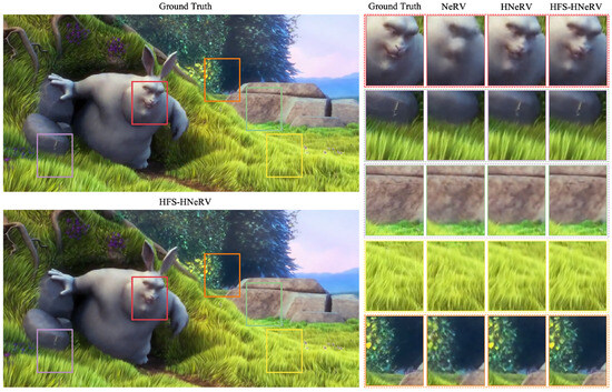
Figure 6.
Visual quality comparison of videos at 0.109 bpp. On the left, we compare one overall video frame generated by HFS-HNeRV with the ground truth. On the right, we compare NeRV, HNeRV, and HFS-HNeRV by extracting and analyzing five patches from the images. It can be observed that HFS-HNeRV consistently outperforms in various aspects, including facial details, small objects (such as the contour of a blade of grass), local region details (such as the texture of rocks and grass), and low-contrast objects (such as a leaf in darkness).
4.3.2. Video Compression
For the video compression task, we employed embedded quantization (8 bits), model quantization (8 bits), and model entropy coding. Figure 7a,b show the rate-distortion performance of HNeRV, HFS-HNeRV, and traditional compression methods (H.264 and H.265), respectively. Although a performance gap remains between NeRV-type methods and conventional compression technologies, HFS-HNeRV outperforms HNeRV, clearly demonstrating that the three proposed components collectively contribute to advancing the performance of NeRV-type architectures.
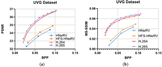
Figure 7.
(a) PSNR(dB) results on UVG dataset. (b) MS-SSIM results on UVG dataset.
4.3.3. Model Complexity
We mainly discuss the model complexity from the perspectives of model parameter count and decoding speed.
For the traditional methods, we directly cite the FPS values of H.264 and H.265 reported in previous work. Since these methods were evaluated using four CPU threads on Intel Xeon 4216 processors, the setup is closer to real-world application scenarios. For the NeRV method, due to the significant performance gap caused by the mobile version of the RTX 3060 GPU, we benchmarked HNeRV and HFS-HNeRV by using the RTX A6000 GPU, whose performance is more comparable to that of a four-core Xeon CPU.
In terms of model complexity, we have made careful efforts to avoid or control the increase in the number of parameters. For instance, the HFS loss does not introduce any additional parameters, and the MSFRP is implemented with bilinear interpolation to minimize parameter overhead. While the introduction of the attention mechanism inevitably adds some parameters, we counteract this by reducing the number of channels across all network layers. This ensures that the total number of model parameters remains consistent across all comparison experiments. The experimental results demonstrate that this trade-off is worthwhile. Our model achieves superior performance under the same parameter budget.
As for decoding speed, compared with traditional compression methods and other NeRV-based approaches, our method shows significantly lower decoding speed (as illustrated in Figure 8). This is primarily due to the additional operations frequently performed within the network—such as wavelet transforms and frequency domain calculations—which introduce higher computational complexity and memory overhead. As a result, the current inference speed of our method is limited.
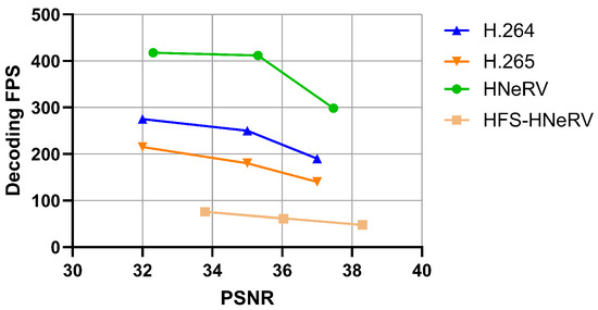
Figure 8.
Decoding FPS comparison.
5. Conclusions
In this paper, we present HFS-HNeRV, a NeRV network optimized for learning high-frequency features within the frequency domain. To support its training, we introduce a specialized loss function designed to target high-frequency features, thereby improving the model’s performance to reproduce fine details such as edges and textures. Specifically, we propose the HFSCM and the HFS loss, which enable the model to more effectively focus on and learn high-frequency information in the frequency domain.
Quantitative results reveal that HFS-HNeRV significantly outperforms other NeRV-based networks, including NeRV, E-NeRV, and HNeRV, achieving improvements in PSNR of +5.75 dB, +4.53 dB, and +1.05 dB, respectively. In terms of visual reconstruction quality, HFS-HNeRV demonstrates superior performance in restoring edge textures and produces images with more cohesive and natural color distributions. Importantly, both HFSCM and HFS loss exhibit a high degree of flexibility, allowing them to be easily integrated into a variety of NeRV architectures, thus offering substantial benefits for tasks related to video compression and reconstruction.
6. Future Work
For future work, we plan to explore the following three aspects:
- The decoding speed of the model needs to be enhanced. The current method still lags behind traditional compression techniques in terms of decoding efficiency, which is a critical factor in practical applications (particularly in scenarios with real-time requirements). To address this limitation, we aim to investigate more efficient frequency domain transformation methods and network simplification strategies to enhance inference speed.
- The model’s adaptability to diverse types of video content needs to be strengthened. As observed from its performance on the UVG dataset, the proposed method remains sensitive to video characteristics, which means that videos featuring rapid motion or complex backgrounds often result in performance degradation. To improve robustness, we will consider incorporating motion estimation mechanisms and enhancing the compression and reconstruction capabilities for high-frequency information.
- We should carefully balance parameter configurations and performance metrics. Given the method’s strict constraints on model size, any newly introduced components or parameter adjustments that significantly increase the number of parameters should be thoroughly evaluated. Therefore, we plan to conduct more comprehensive ablation studies to identify the optimal configuration strategies.
Author Contributions
Conceptualization, J.H.Z. and X.J.L.; methodology, J.H.Z. and X.J.L.; software, J.H.Z.; validation, J.H.Z.; formal analysis, J.H.Z.; investigation, J.H.Z.; resources, J.H.Z. and X.J.L.; data curation, J.H.Z. and X.J.L.; writing—original draft preparation, J.H.Z., X.J.L. and P.H.J.C.; writing—review and editing, J.H.Z., X.J.L. and P.H.J.C.; visualization, J.H.Z. and X.J.L.; supervision, X.J.L. and P.H.J.C.; project administration, X.J.L. and P.H.J.C. All authors have read and agreed to the published version of the manuscript.
Funding
This work was funded by the Vice-Chancellor’s Doctoral Scholarship at Auckland University of Technology, New Zealand.
Data Availability Statement
Data are contained within the article.
Acknowledgments
This article is a revised and expanded version of a paper entitled “HFS-HNeRV: High-Frequency Spectrum Hybrid Neural Representation for Videos”, which was presented at the 6th ACM International Conference on Multimedia in Asia (MMASIA ’24), held in Auckland, New Zealand, on 28 December 2024.
Conflicts of Interest
The authors declare no conflicts of interest.
References
- Tirana, K.; Elmazi, D. 5G Impact on the Flow of Wireless Internet Traffic. In Proceedings of the 2024 International Conference on Computing, Networking, Telecommunications & Engineering Sciences Applications (CoNTESA), Tirana, Albania, 18–19 December 2024; pp. 1–4. [Google Scholar]
- Pratt, W.K.; Kane, J.; Andrews, H.C. Hadamard transform image coding. Proc. IEEE 1969, 57, 58–68. [Google Scholar] [CrossRef]
- Zhang, Z.T.; Yeh, C.H.; Kang, L.W.; Lin, M.H. Efficient CTU-based intra frame coding for HEVC based on deep learning. In Proceedings of the 2017 Asia-Pacific Signal and Information Processing Association Annual Summit and Conference (APSIPA ASC), Kuala Lumpur, Malaysia, 12–15 December 2017; pp. 661–664. [Google Scholar]
- Wang, Y.; Fan, X.; Liu, S.; Zhao, D.; Gao, W. Multi-scale convolutional neural network-based intra prediction for video coding. IEEE Trans. Circuits Syst. Video Technol. 2019, 30, 1803–1815. [Google Scholar] [CrossRef]
- Schneider, J.; Sauer, J.; Wien, M. Dictionary learning based high frequency inter-layer prediction for scalable HEVC. In Proceedings of the 2017 IEEE Visual Communications and Image Processing (VCIP), St. Petersburg, FL, USA, 10–13 December 2017; pp. 1–4. [Google Scholar]
- Wang, Z.; Ma, C.; Liao, R.L.; Ye, Y. Multi-density convolutional neural network for in-loop filter in video coding. In Proceedings of the 2021 Data Compression Conference (DCC), Snowbird, UT, USA, 23–26 March 2021; pp. 23–32. [Google Scholar]
- Huang, Z.; Guo, X.; Shang, M.; Gao, J.; Sun, J. An efficient qp variable convolutional neural network based in-loop filter for intra coding. In Proceedings of the 2021 Data Compression Conference (DCC), Snowbird, UT, USA, 23–26 March 2021; pp. 33–42. [Google Scholar]
- Ho, M.M.; Zhou, J.; He, G.; Li, M.; Li, L. SR-CL-DMC: P-frame coding with super-resolution, color learning, and deep motion compensation. In Proceedings of the IEEE/CVF Conference on Computer Vision and Pattern Recognition Workshops, Seattle, WA, USA, 14–19 June 2020; pp. 124–125. [Google Scholar]
- Lu, G.; Zhang, X.; Ouyang, W.; Chen, L.; Gao, Z.; Xu, D. An end-to-end learning framework for video compression. IEEE Trans. Pattern Anal. Mach. Intell. 2020, 43, 3292–3308. [Google Scholar] [CrossRef] [PubMed]
- Hu, Z.; Xu, D.; Lu, G.; Jiang, W.; Wang, W.; Liu, S. Fvc: An end-to-end framework towards deep video compression in feature space. IEEE Trans. Pattern Anal. Mach. Intell. 2022, 45, 4569–4585. [Google Scholar] [CrossRef] [PubMed]
- Agustsson, E.; Minnen, D.; Johnston, N.; Balle, J.; Hwang, S.J.; Toderici, G. Scale-space flow for end-to-end optimized video compression. In Proceedings of the IEEE/CVF Conference on Computer Vision and Pattern Recognition, Seattle, WA, USA, 14–19 June 2020; pp. 8503–8512. [Google Scholar]
- Fu, L.; Wang, P.; Wang, X. An Improved Neural Network Approach to End-to-end Video Compression. In Proceedings of the 5th International Conference on Computer Information and Big Data Applications, Wuhan China, 26–28 April 2024; pp. 57–61. [Google Scholar]
- Liu, B.; Chen, Y.; Machineni, R.C.; Liu, S.; Kim, H.S. Mmvc: Learned multi-mode video compression with block-based prediction mode selection and density-adaptive entropy coding. In Proceedings of the IEEE/CVF Conference on Computer Vision and Pattern Recognition, Vancouver, BC, Canada, 17–24 June 2023; pp. 18487–18496. [Google Scholar]
- Zou, N.; Zhang, H.; Cricri, F.; Tavakoli, H.R.; Lainema, J.; Aksu, E.; Hannuksela, M.; Rahtu, E. End-to-End Learning for Video Frame Compression with Self-Attention. In Proceedings of the IEEE/CVF Conference on Computer Vision and Pattern Recognition (CVPR) Workshops, Seattle, WA, USA, 13–19 June 2020. [Google Scholar]
- Rippel, O.; Nair, S.; Lew, C.; Branson, S.; Anderson, A.G.; Bourdev, L. Learned Video Compression. In Proceedings of the IEEE/CVF International Conference on Computer Vision (ICCV), Seoul, Republic of Korea, 27 October–2 November 2019. [Google Scholar]
- Wang, S.; Zhao, Y.; Gao, H.; Ye, M.; Li, S. End-to-end video compression for surveillance and conference videos. Multimed. Tools Appl. 2022, 81, 42713–42730. [Google Scholar] [CrossRef]
- Chen, H.; He, B.; Wang, H.; Ren, Y.; Lim, S.N.; Shrivastava, A. Nerv: Neural representations for videos. Adv. Neural Inf. Process. Syst. 2021, 34, 21557–21568. [Google Scholar]
- Li, Z.; Wang, M.; Pi, H.; Xu, K.; Mei, J.; Liu, Y. E-nerv: Expedite neural video representation with disentangled spatial-temporal context. In Computer Vision—ECCV 2022, Proceedings of the 17th European Conference, Tel Aviv, Israel, 23–27 October 2022; Springer: Cham, Switzerland, 2022; pp. 267–284. [Google Scholar]
- Chen, H.; Gwilliam, M.; Lim, S.N.; Shrivastava, A. Hnerv: A hybrid neural representation for videos. In Proceedings of the IEEE/CVF Conference on Computer Vision and Pattern Recognition, Vancouver, BC, Canada, 17–24 June 2023; pp. 10270–10279. [Google Scholar]
- Zhao, J.; Li, X.J.; Chong, P.H.J. HFS-HNeRV: High-Frequency Spectrum Hybrid Neural Representation for Videos. In Proceedings of the 6th ACM International Conference on Multimedia in Asia, Auckland, New Zealand, 3–6 December 2024; pp. 1–7. [Google Scholar]
- Liu, Z.; Mao, H.; Wu, C.Y.; Feichtenhofer, C.; Darrell, T.; Xie, S. A convnet for the 2020s. In Proceedings of the IEEE/CVF Conference on Computer Vision and Pattern Recognition, New Orleans, LA, USA, 18–24 June 2022; pp. 11976–11986. [Google Scholar]
- Woo, S.; Park, J.; Lee, J.Y.; Kweon, I.S. Cbam: Convolutional block attention module. In Proceedings of the European Conference on Computer Vision (ECCV), Munich, Germany, 8–14 September 2018; pp. 3–19. [Google Scholar]
- Liu, Y.; Shao, Z.; Hoffmann, N. Global attention mechanism: Retain information to enhance channel-spatial interactions. arXiv 2021, arXiv:2112.05561. [Google Scholar]
- Mehta, I.; Gharbi, M.; Barnes, C.; Shechtman, E.; Ramamoorthi, R.; Chandraker, M. Modulated periodic activations for generalizable local functional representations. In Proceedings of the IEEE/CVF International Conference on Computer Vision, Montreal, BC, Canada, 11–17 October 2021; pp. 14214–14223. [Google Scholar]
- Strümpler, Y.; Postels, J.; Yang, R.; Gool, L.V.; Tombari, F. Implicit neural representations for image compression. In Computer Vision—ECCV 2022, Proceedings of the 17th European Conference, Tel Aviv, Israel, 23–27 October 2022; Springer: Cham, Switzerland, 2022; pp. 74–91. [Google Scholar]
- Chen, Y.; Liu, S.; Wang, X. Learning continuous image representation with local implicit image function. In Proceedings of the IEEE/CVF Conference on Computer Vision and Pattern Recognition, Nashville, TN, USA, 20–25 June 2021; pp. 8628–8638. [Google Scholar]
- Jiang, C.; Sud, A.; Makadia, A.; Huang, J.; Nießner, M.; Funkhouser, T. Local implicit grid representations for 3d scenes. In Proceedings of the IEEE/CVF Conference on Computer Vision and Pattern Recognition, Seattle, WA, USA, 14–19 June 2020; pp. 6001–6010. [Google Scholar]
- Mildenhall, B.; Srinivasan, P.P.; Tancik, M.; Barron, J.T.; Ramamoorthi, R.; Ng, R. Nerf: Representing scenes as neural radiance fields for view synthesis. Commun. ACM 2021, 65, 99–106. [Google Scholar] [CrossRef]
- Wiegand, T.; Sullivan, G.J.; Bjontegaard, G.; Luthra, A. Overview of the H. 264/AVC video coding standard. IEEE Trans. Circuits Syst. Video Technol. 2003, 13, 560–576. [Google Scholar] [CrossRef]
- Sullivan, G.J.; Ohm, J.R.; Han, W.J.; Wiegand, T. Overview of the high efficiency video coding (HEVC) standard. IEEE Trans. Circuits Syst. Video Technol. 2012, 22, 1649–1668. [Google Scholar] [CrossRef]
- Dong, C.; Loy, C.C.; He, K.; Tang, X. Learning a deep convolutional network for image super-resolution. In Computer Vision–ECCV 2014, Proceedings of the 13th European Conference, Zurich, Switzerland, 6–12 September 2014; Part IV; Springer: Cham, Switzerland, 2014; pp. 184–199. [Google Scholar]
- Kim, J.; Lee, J.K.; Lee, K.M. Accurate image super-resolution using very deep convolutional networks. In Proceedings of the IEEE Conference on Computer Vision and Pattern Recognition, Las Vegas, NV, USA, 27–30 June 2016; pp. 1646–1654. [Google Scholar]
- Shi, W.; Caballero, J.; Huszár, F.; Totz, J.; Aitken, A.P.; Bishop, R.; Rueckert, D.; Wang, Z. Real-time single image and video super-resolution using an efficient sub-pixel convolutional neural network. In Proceedings of the IEEE Conference on Computer Vision and Pattern Recognition, Las Vegas, NV, USA, 27–30 June 2016; pp. 1874–1883. [Google Scholar]
- Shocher, A.; Cohen, N.; Irani, M. “zero-shot” super-resolution using deep internal learning. In Proceedings of the IEEE Conference on Computer Vision and Pattern Recognition, Salt Lake City, UT, USA, 18–23 June 2018; pp. 3118–3126. [Google Scholar]
- Ledig, C.; Theis, L.; Huszar, F.; Caballero, J.; Cunningham, A.; Acosta, A.; Aitken, A.; Tejani, A.; Totz, J.; Wang, Z.; et al. Photo-realistic single image super-resolution using a generative adversarial network. In Proceedings of the IEEE Conference on Computer Vision and Pattern Recognition, Honolulu, HI, USA, 21–26 July 2017; Volume 2017, pp. 4681–4690. [Google Scholar]
- Chan, K.C.; Wang, X.; Yu, K.; Dong, C.; Loy, C.C. Basicvsr: The search for essential components in video super-resolution and beyond. In Proceedings of the IEEE/CVF Conference on Computer Vision and Pattern Recognition, Nashville, TN, USA, 20–25 June 2021; pp. 4947–4956. [Google Scholar]
- Sajjadi, M.S.; Vemulapalli, R.; Brown, M. Frame-recurrent video super-resolution. In Proceedings of the IEEE Conference on Computer Vision and Pattern Recognition, Salt Lake City, UT, USA, 18–23 June 2018; pp. 6626–6634. [Google Scholar]
- Xue, T.; Chen, B.; Wu, J.; Wei, D.; Freeman, W.T. Video enhancement with task-oriented flow. Int. J. Comput. Vis. 2019, 127, 1106–1125. [Google Scholar] [CrossRef]
- Kim, T.H.; Sajjadi, M.S.; Hirsch, M.; Scholkopf, B. Spatio-temporal transformer network for video restoration. In Proceedings of the European Conference on Computer Vision (ECCV), Munich, Germany, 8–14 September 2018; pp. 106–122. [Google Scholar]
- Tian, Y.; Zhang, Y.; Fu, Y.; Xu, C. Tdan: Temporally-deformable alignment network for video super-resolution. In Proceedings of the IEEE/CVF Conference on Computer Vision and Pattern Recognition, Seattle, WA, USA, 14–19 June 2020; pp. 3360–3369. [Google Scholar]
- Ying, X.; Wang, L.; Wang, Y.; Sheng, W.; An, W.; Guo, Y. Deformable 3d convolution for video super-resolution. IEEE Signal Process. Lett. 2020, 27, 1500–1504. [Google Scholar] [CrossRef]
- Kim, S.Y.; Lim, J.; Na, T.; Kim, M. Video super-resolution based on 3D-CNNS with consideration of scene change. In Proceedings of the 2019 IEEE International Conference on Image Processing (ICIP), Taipei, Taiwan, 22–25 September 2019; pp. 2831–2835. [Google Scholar]
- Liu, H.; Zhao, P.; Ruan, Z.; Shang, F.; Liu, Y. Large motion video super-resolution with dual subnet and multi-stage communicated upsampling. Proc. AAAI Conf. Artif. Intell. 2021, 35, 2127–2135. [Google Scholar] [CrossRef]
- Zhu, X.; Li, Z.; Zhang, X.Y.; Li, C.; Liu, Y.; Xue, Z. Residual invertible spatio-temporal network for video super-resolution. Proc. AAAI Conf. Artif. Intell. 2019, 33, 5981–5988. [Google Scholar] [CrossRef]
- Isobe, T.; Jia, X.; Gu, S.; Li, S.; Wang, S.; Tian, Q. Video super-resolution with recurrent structure-detail network. In Computer Vision—ECCV 2020, Proceedings of the 16th European Conference, Glasgow, UK, 23–28 August 2020; Part XII; Springer: Cham, Switzerland, 2020; pp. 645–660. [Google Scholar]
- Goodfellow, I.J.; Pouget-Abadie, J.; Mirza, M.; Xu, B.; Warde-Farley, D.; Ozair, S.; Courville, A.; Bengio, Y. Generative adversarial nets. In Proceedings of the 27th International Conference on Neural Information Processing Systems, Lake Tahoe, NV, USA, 5–10 December 2013; pp. 2672–2680. [Google Scholar]
- Liu, H.; Ruan, Z.; Zhao, P.; Dong, C.; Shang, F.; Liu, Y.; Yang, L.; Timofte, R. Video super-resolution based on deep learning: A comprehensive survey. Artif. Intell. Rev. 2022, 55, 5981–6035. [Google Scholar] [CrossRef]
- Baniya, A.A.; Lee, T.K.; Eklund, P.W.; Aryal, S. A survey of deep learning video super-resolution. IEEE Trans. Emerg. Top. Comput. Intell. 2024, 8, 2655–2676. [Google Scholar] [CrossRef]
- Wang, Z.; Chen, J.; Hoi, S.C. Deep learning for image super-resolution: A survey. IEEE Trans. Pattern Anal. Mach. Intell. 2020, 43, 3365–3387. [Google Scholar] [CrossRef] [PubMed]
- Rhee, H.; Jang, Y.I.; Kim, S.; Cho, N.I. LC-FDNet: Learned lossless image compression with frequency decomposition network. In Proceedings of the IEEE/CVF Conference on Computer Vision and Pattern Recognition, New Orleans, LA, USA, 18–24 June 2022; pp. 6033–6042. [Google Scholar]
- Gao, G.; You, P.; Pan, R.; Han, S.; Zhang, Y.; Dai, Y.; Lee, H. Neural image compression via attentional multi-scale back projection and frequency decomposition. In Proceedings of the IEEE/CVF International Conference on Computer Vision, Montreal, BC, Canada, 11–17 October 2021; pp. 14677–14686. [Google Scholar]
- Li, H.; Li, S.; Dai, W.; Li, C.; Zou, J.; Xiong, H. Frequency-aware transformer for learned image compression. arXiv 2023, arXiv:2310.16387. [Google Scholar]
- Pan, Z.; Cai, J.; Zhuang, B. Fast vision transformers with hilo attention. Adv. Neural Inf. Process. Syst. 2022, 35, 14541–14554. [Google Scholar]
- Porwik, P.; Lisowska, A. The Haar-wavelet transform in digital image processing: Its status and achievements. Mach. Graph. Vis. 2004, 13, 79–98. [Google Scholar]
- Kidner, D.; Dorey, M.; Smith, D. What’s the point? Interpolation and extrapolation with a regular grid DEM. In Proceedings of the Fourth International Conference on GeoComputation, Fredericksburg, VA, USA, 25–28 July 1999. [Google Scholar]
Disclaimer/Publisher’s Note: The statements, opinions and data contained in all publications are solely those of the individual author(s) and contributor(s) and not of MDPI and/or the editor(s). MDPI and/or the editor(s) disclaim responsibility for any injury to people or property resulting from any ideas, methods, instructions or products referred to in the content. |
© 2025 by the authors. Licensee MDPI, Basel, Switzerland. This article is an open access article distributed under the terms and conditions of the Creative Commons Attribution (CC BY) license (https://creativecommons.org/licenses/by/4.0/).