Abstract
Accurate evaluation of the operational status of smart meters, as the critical interface between the power grid and its users, is essential for ensuring fairness in power transactions. This highlights the importance of implementing rotation management practices based on meter status. However, the traditional expiration-based rotation method has become inadequate due to the extended service life of modern smart meters, necessitating a shift toward status-driven targeted management. Existing multifactor comprehensive assessment methods often face challenges in balancing accuracy and interpretability. To address these limitations, this study proposes a novel method for analyzing the status of smart meter groups using an interpretable random forest model. The approach incorporates an expert-knowledge-guided grouping assessment strategy, develops a multi-source heterogeneous feature set with strong correlations to meter status, and enhances the random forest model with the SHAP (SHapley Additive exPlanations) interpretability framework. Compared to conventional methods, the proposed approach demonstrates superior efficiency and reliability in predicting the failure rates of smart meter groups within distribution network areas, offering robust support for the maintenance and management of smart meters.
1. Introduction
The smart energy meter is an intelligent power measurement instrument, and accurately assessing its operational status is essential for ensuring the fairness of power transactions. The smart meters targeted in this study are primarily single-phase meters for residential use. These meters are equipped with core functionalities to support status monitoring: they feature high-precision metering modules and timing systems while also recording operational events and real-time monitoring data. These meters are fully integrated into the SMART-METERING system—a centralized platform for smart grid data management—acting as end-node sensors that upload real-time and historical data to the system via bidirectional communication. This integration enables the system to aggregate multi-source data, laying the groundwork for the state monitoring and analysis of meters.
While individual electricity usage profiles vary, meter faults can lead to unfair billing—either overcharging users or undercharging—leading to losses for grid companies. Therefore, management of smart meters’ operation quality is necessary. While smart meters transmit basic diagnostic data to billing servers automatically, this process has critical limitations:
- (1)
- Some failures cannot be detected by automatic systems and rely on user feedback, leading to delayed or inaccurate failure identification;
- (2)
- Automatic data transmission may generate misjudgments and correcting these individually requires substantial manpower and resources;
- (3)
- Traditional expiration-based rotation often results in unnecessary removal of non-faulty meters, wasting materials and labor.
According to the Measures for the Supervision and Management of Electricity Meter Quality by the State Grid Corporation Limited, to address the issues mentioned above, the corporation implements a strategy of periodic inspections and mandatory rotation upon expiration to ensure the stable operation of smart meters. However, this approach lacks comprehensive management of the entire lifecycle of the device’s operation [1,2]. In recent years, advancements in power meter technology have generally extended the service life of these meters. Consequently, the rotation management strategy consumes significant human, material, and financial resources. To enhance the precision of smart energy meter management and transition from a planned maintenance mode based on on-site inspections to a state maintenance mode based on operational status, there is an urgent need to investigate the key technologies for assessing the condition of smart energy meters [3,4,5].
The current methods for assessing the condition of smart energy meters are primarily categorized into two types: univariate analysis and multivariate analysis. The univariate analysis method typically focuses on a specific operational index of the energy meter, predicting its operational status based solely on this single index, such as the online rate of the energy meter. For instance, Cheng et al. demonstrated that when analyzing operating errors in power metering devices, a single-fault characteristic—such as voltage abnormalities or current loss—can be utilized to quickly identify the issue [6]. Additionally, the state awareness technique based on accelerated degradation test data, as shown by Ma et al., further highlights the effectiveness of single-factor analysis in particular scenarios [7]. Chen et al. developed a Wiener process approach, which models battery degradation through stochastic processes. This provides ‘white-box’ interpretability via physical failure mechanisms [8]. However, its unidimensional predictions struggle to address complex multi-fault scenarios. This method provides clear causality and interpretability. However, it also contains notable limitations. On one hand, a single factor often fails to comprehensively represent the actual state of the energy meter in a complex operating environment. On the other hand, univariate analysis cannot capture the synergistic effects of environmental factors, which may easily lead to misjudgments [9].
In contrast, the multivariate analysis provides a more thorough assessment of energy meter status by integrating data from multiple sources. Luo et al. developed a smart energy meter state inspection and evaluation system that significantly enhances evaluation accuracy by constructing a framework based on multidimensional indicators [10]. The entropy weight-normal cloud model proposed by Gao et al. determines the weights of the assessment indicators using the entropy weight method and addresses the quantitative challenges associated with multifactor assessment indicators through the normal cloud model [11]. The remote online evaluation system designed by Zhang et al. effectively integrates multifactor data using a decoupled evaluation algorithm [12]. However, these methods face challenges related to interpretability: firstly, complex feature interactions complicate the interpretation of results; secondly, while multivariate analysis improves analytical accuracy, the internal mechanisms of most models still exhibit characteristics of a “black box”.
To balance assessment accuracy and interpretability, the data-driven monitoring method proposed by Lai decomposes and refines the complex problem into multiple interpretable sub-modules through component-by-component comparisons [13]. However, this method primarily focuses on component factors and does not comprehensively consider other key elements, such as operating environment factors. Yu et al. applied the reverse feature elimination (RFE) method for data dimensionality reduction to identify five main variables affecting the online rate [14]. However, the model they selected was linear and could not account for the complex interrelationships among the various factors.
Key measurable quantities for smart meter status include intrinsic metering error, daily timing error, cumulative failure rate, operation time, events, environmental interference indicators and real-time monitoring data of current, voltage, power and electricity. This paper focuses on observing intrinsic error, cumulative failure rate of grouped meters, operation time and events as core indicators to reflect operational status, leaving out the real-time monitoring data due to its extremely large volume. Based on the above data, in light of the challenges associated with balancing assessment accuracy and interpretability in multi-source data fusion for the comprehensive evaluation of power equipment status, this paper proposes a group smart meter status analysis method based on an interpretable random forest model. It introduces an expert-knowledge-guided assessment strategy for the group status analysis of smart meters. Consequently, a high-correlation feature set is constructed for the state of power meters by integrating multi-source heterogeneous data. Furthermore, a random forest enhancement model utilizing the SHAP interpretability framework is developed to extract key features from the complex coupled feature set, thereby improving the model’s evaluation accuracy. By predicting failure risks, we enable proactive maintenance to preserve accuracy of measurement, safeguarding transaction fairness.
2. Background and Related Technologies
In this paper, we will utilize the random forest model, the Isolation Forest anomaly detection method, the state assessment related feature construction method, and the SHAP interpretability framework. The relevant techniques and principles will be introduced in the following sections.
2.1. Random Forest Model
Random forest is an ensemble learning method based on decision trees that aims to enhance model performance by constructing multiple weak learners and aggregating their predictions. The algorithm introduces dual randomness in the training of each decision tree: first, a random subset of features is selected from the feature space (typically the square root of the total number of features), and then the optimal split is determined using metrics such as information gain or Gini impurity during node splitting. For classification tasks, a majority voting mechanism is employed, while for regression tasks, mean aggregation is utilized. This random feature selection mechanism effectively reduces the correlation between decision trees. Meanwhile, aggregation applies the law of large numbers. Together, they ensure model stability [15].
2.2. Isolated Forest Model
Isolation Forest, constructed from binary trees, is an unsupervised, nonparametric method for detecting anomalies in multivariate data [16]. As a variant of the random forest model, the fundamental concept of Isolation Forest is to repeatedly partition the data space using random hyperplanes until only one data point remains in each subspace. Since anomalous data is typically sparsely distributed, Isolation Forests can effectively isolate them with fewer cuts, thereby facilitating anomaly detection. The formula for calculating the sparsity (anomaly score) is as follows:
where E(h(x)) represents the average path length of sample x across all isolated trees, c(n) is the normalization factor that indicates the average path length estimate of the binary tree based on n samples, and n denotes the number of samples in the training dataset. The isolated forest algorithm does not rely on similarity measures, density, or other indicators to describe the differences between samples; instead, it directly characterizes the degree of sparsity and filters out a specified proportion of outliers. This approach makes it suitable for data preprocessing in machine learning, ultimately enhancing the quality of the dataset.
2.3. Theil Index
The Theil index was proposed by the Dutch economist Henri Theil [17], based on information theory, and was initially utilized to study income disparities between countries. The Theil index effectively captures fairness by enabling a detailed division of global differences into variations across time, regions, and hierarchical scales, thereby facilitating a deeper analysis of the causes of inequality [18]. The formula for the Theil index is as follows:
where Ti is the Theil index of the ith region, Ti,j is the Theil index of the jth secondary region of the ith region, Pi,j is the population of the jth secondary region of the ith region, Pi is the population of the ith region, P is the total population, Fi,j is the income of the jth secondary region of the ith region, Fi is the income of the ith region, and F is the total revenue.
When “Revenue” is converted to failure rate, and “Region” and “Secondary Region” are converted to manufacturer and production batch, the Theil index can effectively reflect the differences in failure rates among various manufacturers and batches.
2.4. SHAP Interpretability Framework
SHAP (SHapley Additive exPlanations) is a model-independent method for explaining machine learning predictions. It quantifies the contribution of individual features to a specific prediction and aggregates these local results to provide a comprehensive explanation of the model [17]. SHAP is rooted in Cooperative Game Theory, where Shapley regression values, Shapley sampling values, and Quantitative Input Influence (QII) contributions are computed through weighted averaging over subsets of features.
where {x1, …, xp}\{xj} represents the set of all remaining features excluding the jth feature, S is a subset of this set, |S| denotes the number of nonzero elements in S, and p is the total number of features in the complete feature set [19].
3. Proposed Methods
The challenge of analyzing smart meter states involves integrating failure data from meters, which may vary in data types and degrees of correlation, with a knowledge graph to create display features that accurately represent the failures of multiple meters. Additionally, a significant challenge is the precise quantification of the relationships among numerous features that differ in modality, correlation strength, and data balance, among other factors, in relation to the failures [20].
This paper integrates expert knowledge with knowledge mapping to analyze the significance of raw data. It proposes a grouping assessment method that combines production batch and distribution network information, and categorizes the data into three types: verification-related, production-related, and deployment-related. Targeted processing is then applied to each category, transforming various types of raw data into a unified set of failure-related features. For the multimodal failure features, data anomalies are addressed using Isolation Forests. Subsequently, a decision tree ensemble learning model, specifically the random forest, is employed to conduct research on data-driven failure rate modeling for smart energy meters. The specific process is illustrated in Figure 1.
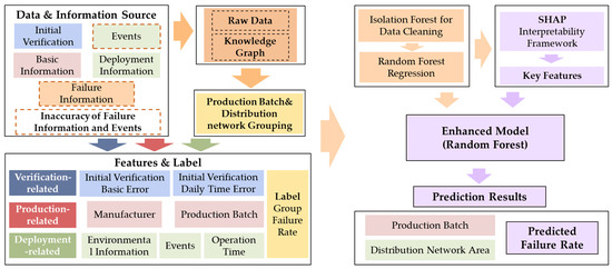
Figure 1.
Flow chart of intelligent energy meter state analysis method.
Figure 1 visually depicts this process, explicitly mapping the flow from raw inputs through feature engineering, data cleaning, and model training to the final output: predicted failure rates for meter groups defined by production batch and distribution network area. The figure highlights how failure information risks inaccuracies, with event data susceptible due to environmental and communication disruptions, underscoring the importance of robust feature engineering and model design to mitigate these interferences.
4. State Feature Construction
Constructing state characteristic parameters involves two key processes: extraction and correlation analysis. In the extraction phase, theoretical analysis and expert experience are utilized to identify the physical quantities associated with the label parameter, specifically the cumulative failure rate. Subsequently, state characteristic parameters that effectively represent these quantities are developed, facilitating the construction of features necessary for knowledge fusion. In the correlation analysis phase, the actual values of each state characteristic parameter and the label parameter are examined. This analysis investigates the relationships between state characteristic parameters, as well as the relationships between state characteristic parameters and failure labels. The objective is to analyze the characteristics of the feature dataset, which will inform subsequent data cleaning and model construction. The latter is based on the actual values of each state feature parameter and label parameter, and it conducts correlation analysis between state feature parameters, as well as between state feature parameters and failure labels. This aims to analyze the characteristics of the feature dataset, enabling more effective data processing and model development.
4.1. Smart Energy Meter Evaluation Group Methods
Compared to traditional state analysis methods that focus on isolated individuals, this paper introduces an expert-knowledge-guided smart meter grouping method. In this approach, the smallest unit defined by intrinsic attributes is the production batch, while the smallest unit of the operating environment is the distribution network. Grouping is constructed based on the unique combination of the batch and the distribution network area, which serves as the research object for the state analysis method. This grouping method offers several advantages: (1) it reduces the sample size while incorporating all meter information, thereby enhancing model efficiency; (2) production batch and distribution network account for differences in production and installation, making the model more interpretable; and (3) the model emphasizes the characteristics of the meter group, thereby minimizing the impact of abnormal samples. Based on this grouping rule, the extraction of smart meter state label parameters and the construction of state feature parameters are carried out next.
4.2. Smart Energy Meter State Feature and Label Extraction
Sorting through the existing data, the current data sources include asset information, comprehensive performance inspection data, initial verification data, failure classification data, installation information, operational data, and operational event records. The extractable features are categorized into three types: verification-related, production-related, and deployment-related, each labeled with the corresponding failure rate. The following section outlines the selection and calculation process for each type of feature and label.
4.2.1. Verification-Related Features
The data source for verification-related features is the initial verification data, which reflects the meter’s initial metrological performance and, to some extent, the level of manufacturing technology employed in its production. The verification features possess the following characteristics:
- (1)
- Features Associated with the Intrinsic error from the Initial Verification Data
From the intrinsic error term of the initial verification data, power factors of 0.5 L and 1.0 are considered as the working conditions. For each group, statistical features are extracted from the data of the entire meter, including the mean value (μ), standard deviation (σ), skewness (Skew), kurtosis (Kurt), and the range of extreme deviations (Range). The mathematical expressions for the features are as follows:
where ξ is the intrinsic error of smart meters in a valuation group, N is the number of meters for the valuation group, μ(ξ) is the mean value within the group, σ(ξ) is the standard deviation within the group, Skew(ξ) is the skewness within the group, Kurt(ξ) is the kurtosis within the group, and Range(ξ) is the extreme deviation within the group.
- (2)
- Features Associated with the Daily Timing Error of the First Verification Data
From the daily timing error term of the initial verification data, statistical features were extracted for each group, including the mean value, standard deviation, skewness, kurtosis, and extreme deviation. The formulas used for these calculations were consistent with those applied to the intrinsic error. The mathematical expressions for the features are as follows:
where ξclock is the intrinsic error of smart meters in a valuation group, N is the number of meters for the valuation group, μ(ξclock) is the mean value within the group, σ(ξclock) is the standard deviation within the group, Skew(ξclock) is the skewness within the group, Kurt(ξclock) is the kurtosis within the group, and Range(ξclock) is the extreme deviation within the group.
4.2.2. Production-Related Features
The data source for the production-related features includes asset information, comprehensive performance testing data, and failure classification data. These sources reflect the attribute information of the meter and indicate its status through the overall group attributes of the meter manufacturer and batch. The production-related features possess the following characteristics:
- (1)
- Features Associated with Manufacturers’ Information
Based on the failure statistics, the cumulative failure rate Ri is calculated for each manufacturer i. The mathematical expression for the feature is as follows:
where Ri is the cumulative failure rate of smart meters produced by manufacturer i, Pi is the total number of smart meters produced by manufacturer i, and Fi is the number of failures in the total meters produced by manufacturer i.
- (2)
- Features Associated with Production Batch Information
The cumulative failure rate Ri,j for each production batch j is calculated based on the failure statistics. The mathematical expressions for the features are as follows:
where Ri,j is the cumulative failure rate of smart meters in batch j, which is produced by manufacturer i. Pi,j is the total number of smart meters in batch i, and Fi,j is the number of failures in the total batch.
- (3)
- Theil Index for Manufacturer and Production Batch Information
Manufacturers and production batches, as two distinct levels of division indicators in energy meter production, can be utilized to quantify the differences in failures among various manufacturers, between batches from the same manufacturer, and between batches from different manufacturers through the application of the second level of the Theil index.
Taking manufacturers i as a ‘region’, and different batches of the same manufacturer j as a ‘secondary region’, then the Theil index Ti between different manufacturers i is as follows:
where Pi is the total number of installations of manufacturer i, and Fi is the number of failures therein; Pi,j is the number of installations of batch j in manufacturer i, and Fi,j is the number of failures therein.
Furthermore, the Theil index Ti,j of different batches produced by same manufacturer is as follows:
The Theil index Ti between different manufacturers i, and the Theil index Ti,j for different batches j of the same manufacturer i are derived from the failure rates of the manufacturers and production batches.
4.2.3. Deployment-Related Features
The data sources for the deployment-related features include installation information and anomaly events, which reflect the operational environment and the dynamic status of the meter.
- (1)
- Features Associated with Operation Time
The mathematical expressions for the features associated with the average operation time (in years) of all meters, including both failed and normal ones, within each category up to the present time are as follows:
where N is the number of meters in the group and Topeation,i is the running time of any meter in the evaluation group.
- (2)
- Features Associated with Environmental Information
There are two types of environmental information: one pertains to the correlation between temperature and relative humidity [21], while the other relates to the correlation of salt fog in the atmosphere.
As for the temperature and relative humidity, the features are calculated by city. First, identify the installation city. Then, compute each group’s total runtime. Finally, determine the percentage of time exceeding temperature/humidity thresholds (both measured in hours), tT and tRH. This analysis will characterize the impact of the smart meter under high-temperature conditions, with the threshold values selected from GB/T 4798.3-2023 [22]. The mathematical expressions are as follows:
where toverT, toverRH is the time of exceeding the threshold value, calculated as hours.
As for the salt fog, the literature indicates that it is correlated with the distance from the coastline [23,24]. Therefore, using geographic information data, the distance between the area and the coastline, denoted as D (km), is calculated as an environmental feature, which is directly derived from geographic information.
- (3)
- Features Associated with Anomaly Events
The operational events can be categorized into three types: power outage events, battery under-voltage events, and over-current events. Power outage events significantly impact the stable operation of both the clock and the battery [25]. Notably, the smart meters evaluated in this study are primarily residential meters with a rated voltage of 220 V and rated currents of 40 A or 60 A. When the measured current exceeds this range, it may cause inaccuracies or program disorder, which is why over-current events are included as a key feature. Over-current events usually lead to potential damage or disorder of the meter, while under-voltage events indicate a deteriorating battery status. Collectively, these events offer valuable insights into the condition of the meter.
For outage events, the average cumulative outage time (measured in hours) and the average number of outages (measured in occurrences) for all meters within each group, up to the current group, are calculated as characteristic features. The mathematical expressions are as follows:
where is the group average cumulative outage time, Toutage,i is the cumulative power outage time of any meter in the group, is the group average number of outage events, noutage,i is the cumulative outage time of any meter in the group, and N is the number of meters in the group. For battery under-voltage events, calculate the average number of occurrences and the average frequency (in occurrences per year) of these events for all meters within each group. The mathematical expressions are as follows:
where te1i is the last occurrence of undervoltage for the meter, te0i is the first occurrence of undervoltage for the meter, and nundervoltage, i is the number of undervoltage occurrences between two moments of the smart meter. For overcurrent events, the total number of occurrences (units) and the average frequency (units per year) of all meter overcurrent events within each group are calculated as features. The mathematical expressions are as follows:
where to1i is the moment when the last overcurrent occurs in the grouped meters, to0i is the moment when the first overcurrent occurs in the grouped meters, and novercurrent, i is the number of over-currents of any one meter in the group.
4.2.4. Smart Meter State Label Extraction
For the analyzed object, specifically the group of distribution network areas and production batches, the cumulative failure rate of all smart meters within this group—calculated since their connection to the grid—is recorded and designated as a labeling parameter. This parameter effectively reflects the overall operational status of all smart meters in the group. The mathematical expressions for the label are as follows:
where L(Area, Batch) is the fault rate label of the smart meter evaluation group, N(Area, Batch) is all the installed grid-connected and operating meters of the group, and F(Area, Batch) is the total number of faulty meters in the subgroup after grid-connected and operating.
5. State Characterization
Qualitative and quantitative analyses of the constructed state feature covariates can elucidate the distribution characteristics of these features. This analysis is beneficial for data cleaning and model development [26]. In the following section, the state features will be examined using graphical representations, correlation analysis, and other methods.
5.1. Distribution Analysis of Smart Energy Meter State Characteristics
In order to illustrate the distribution of various features of the smart energy meter, the univariate distribution is visualized by violin plots.
A violin plot is a data visualization chart that combines the characteristics of box-and-whisker plots and kernel density plots. It is often used to illustrate the distribution of data, making it particularly useful for comparing differences in distribution among various groups. After normalizing the state features, the violin plot is presented, as shown in Figure 2.
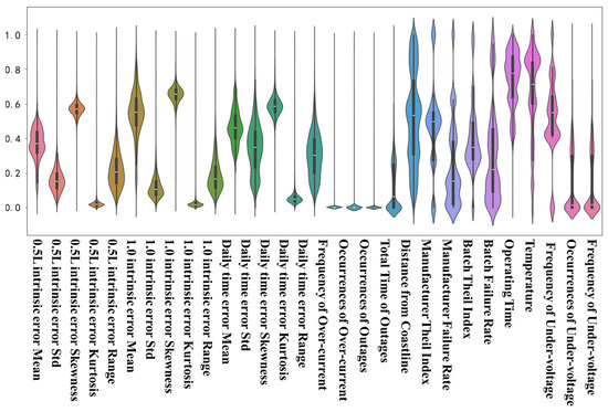
Figure 2.
Violin diagram of state characteristics, label distribution.
Before generating the violin plots in Figure 2, all state features underwent a min–max normalization process. This step scales each feature to a uniform range of [0, 1]. This normalization addresses the issue of inconsistent value ranges among different features. By standardizing the scale, it ensures fair visual comparison of distribution shapes across all features, eliminating biases caused by absolute value differences. The normalized data retains the original distribution characteristics (e.g., skewness, kurtosis) while enabling direct visual alignment in the violin plot.
From the specific distribution of the piano diagram, it can be seen that they have the following three types of distribution:
- (1)
- Sparsely Distributed
Features such as “distance from the coast,” “manufacturer’s failure rate,” “manufacturer’s Theil index,” “production batch failure rate,” “batch Theil Index,” and “temperature and relative humidity” exhibit scattered distributions. Their violin shapes are broad and irregular, indicating high variability across groups. This suggests these features are sensitive to external factors and may act as “differentiators” for failure risk. For example, “temperature and relative humidity” varies significantly across groups as the meters are deployed in various climate zones—high-temperature and high-humidity areas (e.g., southern regions) accelerate circuit degradation, while dry and cool areas (e.g., northern regions) reduce such risks, leading to distinct distribution patterns.
- (2)
- Long-Tailed Concentrated Near Zero
Features including “the kurtosis of the intrinsic error at a 0.5 L power factor,” “the kurtosis of the intrinsic error at a 1.0 power factor,” “the kurtosis of daily timing error,” “the labeling of the failure rate,” and “the frequency of under-voltage” show violin shapes that are narrow near zero but extend into long tails. This indicates most groups have values close to the mean, but a small number of outliers drive extreme deviations. For instance, the long tail in “the labeling of the failure rate” aligns with real-world scenarios where most meter groups have low failure rates, while a few high-risk groups skew the distribution. These outliers require careful handling during modeling to avoid overfitting.
- (3)
- Concentrated Distributions with Few Outliers
The remaining state features display compact violin shapes with minimal tail extension, indicating stable and consistent values across groups. Their low variability suggests they contribute less to distinguishing failure rates individually but may enhance model robustness when combined with other features. For example, “mean of intrinsic error at 0.5 L power factor” is concentrated because smart meters undergo strict initial verification, ensuring most meet basic accuracy standards, with only occasional outliers due to individual meter defects.
For a feature set with such multimodal distributions, we should select appropriate outlier-cleaning methods and regression algorithms to prevent the model from overfitting or becoming stuck in local optima. Additionally, this type of multimodal distribution will also affect model interpretation; when explaining the impact of features on the model, we should consider their distribution characteristics.
5.2. Correlation Analysis Between Features
In order to analyze the relationship between various features in the data and to gain a deeper understanding of the strength of correlation among these features, features with absolute correlation coefficients greater than 0.4 were plotted as undirected graphs. This visualization reflects the clustering structure of correlations between the state features.
The direct and indirect associations among various related state features are illustrated in Figure 3. Certain state features that form clusters, such as the 1.0 intrinsic error standard deviation, 0.5 L intrinsic error standard deviation, 1.0 intrinsic error range, and 0.5 L intrinsic error range, suggest that these features may play similar roles in the data or be influenced by comparable factors. The features corresponding to the nodes within the same cluster that exhibit the most connections with other nodes can be considered key features. Examples include distance from coastline, 0.5 L intrinsic error range, manufacturer’s failure rate, and batch Theil index, as depicted in the figure. These key features may have the capacity to represent those at other nodes while retaining the most information and simplifying the set of state features as much as possible.
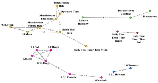
Figure 3.
Diagram of correlation groups of state characteristics.
5.3. Correlation Analysis of State Features and Labels
In order to comprehend the extent of the correlation between various state features and failure rate labels, horizontal bar charts illustrating the absolute values of the correlation coefficients for each state feature and the corresponding failure rate labels are presented, as shown in Figure 4.
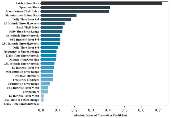
Figure 4.
Histogram of correlation coefficients between state features and labels.
Figure 4 illustrates the ranking of the correlation coefficients of various state features in relation to the failure rate label. The features exhibiting the strongest correlations are the batch failure rate (0.72), operation time (0.41), and Theil index (−0.41). As shown in Figure 4, the top features all demonstrate varying degrees of univariate correlation with the label.
It can be observed from the correlation analysis above that the selected features were partly validated to have significant correlations with the failure rate label, confirming their predictive value. For example, the batch failure rate (r = 0.72) directly reflects historical quality performance, while operation time (r = 0.41) aligns with the physical degradation law of electrical components. However, some features are advised to be taken into consideration even though these have a low value of linear correlation coefficient, as experts point out that they influence the quality of meters’ operation, which is concluded from the experience, structure and principle of smart meters. Those features are then assumed that have nonlinear correlations with failure.
According to the distribution visualization and correlation analysis presented above, it can be concluded that the state features exhibit multimodal distributions. Furthermore, the correlations between the features and the failure labels, as well as among the features themselves, are coupled rather than exhibiting direct univariate correlations. Therefore, in this paper, we will establish a state analysis model that accounts for multifactorial coupling effects, based on a random forest model, to enhance the model’s predictive performance.
6. State Analysis Modeling
In this paper, the state analysis model utilizes a random forest regressor for regression learning, using the grouped failure rate as the target and various extracted state features as inputs. This approach predicts the failure rate of the smart meter in a group and establishes a comprehensive global state analysis model that integrates all features.
6.1. Data Cleaning and Preprocessing
After extracting various types of state features, the first step is to identify and eliminate abnormal outliers. Due to the high dimensionality of the state feature parameters and their complex intercorrelations, as illustrated in Figure 2, a significant portion of the distribution characteristics of these parameters does not conform to a normal distribution. Therefore, it is inappropriate to use conventional methods such as Z-scores or quartile screening for outlier detection. Additionally, cleaning each state feature individually is not advisable due to their complex correlation. Instead, a comprehensive approach that accommodates various distributions should be employed for outlier removal. Consequently, the Isolation Forest algorithm is utilized for detecting outliers, with the screening proportion set at 10% to clean the entire dataset.
After data cleaning, the various types of state features, which possess different magnitudes and value domains, are scaled to a uniform interval of [0, 1] through normalization. This process mitigates the effects of scale and distribution discrepancies on the model. To further enhance model performance, we will identify the optimal parameters by employing cross-validation with a validation set and utilizing grid search for automated tuning. Finally, we will assess the model’s predictive performance on the test set.
6.2. Validation of the Group Assessment Approach
Using both grouped and traditional single-evaluation approaches, the same data cleaning and feature construction methods were applied. A random forest model with automatic parameter optimization was utilized for single-table classification evaluation, and the predictions were compared with the grouped predictions presented in Table 1.

Table 1.
Prediction results of the model.
The root-mean-square error (RMSE) of the test set label predictions, after normalization for the group assessment method, is 0.00472, and the goodness of fit is 0.860. This indicates that the error between the predicted label values and the actual label values is minimal, demonstrating that the model exhibits strong regression capabilities and effective predictive performance. In contrast, the evaluation of the test set using the single-meter assessment approach reveals an accuracy of less than 50%, which is insufficient for precise meter state analysis.
We applied automatic parameter optimization uniformly. Nevertheless, the single-form assessment method showed substantial overfitting. This issue can be attributed to the presence of a substantial amount of anomalous data within the single-form assessment method (as illustrated in Figure 2), which resulted in poor model generalization capabilities. This further underscores the effectiveness of the grouped assessment approach.
6.3. Comparison of Various Model Assessment Approaches
A comparison of the random forest model utilized in this paper with other models on the test set is presented in Table 2. Additionally, a scatter plot illustrating the regression of the labels for both the training and test sets is displayed in Figure 5. The dashed line represents the ideal distribution, indicating perfectly accurate regression.
Table 2.
The prediction results of different models on the test set.
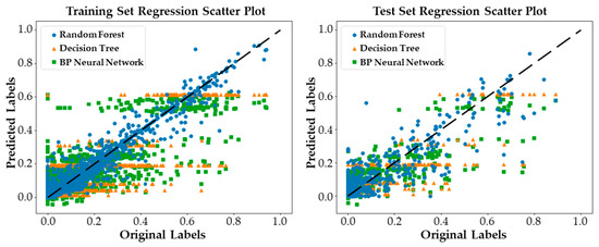
Figure 5.
Model regression scatter plot.
For the various types of features proposed in this paper, the application of random forests demonstrates superior performance in both testing and fitting compared to backpropagation (BP) neural networks and decision trees, as illustrated in Table 2.
7. State Analysis Model Interpretation and Enhancement
SHAP analysis is performed on the established state analysis model using the complete dataset, and the SHAP value for each feature in every sample is calculated to gain insights.
The feature importance graph, illustrated in Figure 6, is accompanied by a feature swarm plot presented in Figure 7. In Figure 6, the horizontal axis represents the average contribution of each feature to the failure rate label. In contrast, Figure 7 displays the contribution of each feature to the failure rate label for individual samples along the horizontal axis. The intensity of the scatter color reflects the magnitude of the corresponding feature value.
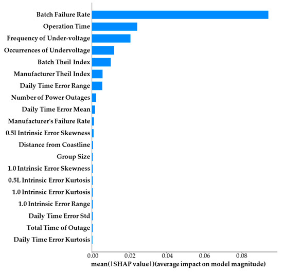
Figure 6.
SHAP feature-importance-ranking diagram.
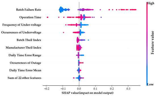
Figure 7.
SHAP bee swarm plot.
As illustrated in Figure 6, the running time, manufacturer and batch failure rate, Theil index, and frequency and occurrences of undervoltage are the most significant features. These findings align with the results produced by the model. The model’s accuracy is significantly compromised when these features are absent, indicating that they contribute the most to the model’s performance. Notably, with a relatively low correlation coefficient, frequency and occurrences of undervoltage are considered important, validating experts’ consultation mentioned in Section 5.3.
As illustrated in Figure 7, the feature swarm diagram reveals that the features of batch failure rate, undervoltage frequency, kurtosis of the 1.0 power factor measurement error, and the number of outages exhibit a clear distinction in their influence on the grouping failure rate. For instance, lower kurtosis values affect model outputs positively. This effect increases the predicted group failure rate. Conversely, when the number of outages is low, it has a minimal effect on the model output, indicating that a lower number of outages does not contribute to the grouping failure rate. However, as the number of outages increases, the grouping failure rate also rises.
To verify the effectiveness of SHAP in extracting feature importance and to demonstrate its impact on prediction accuracy, the previously mentioned random forest model is utilized. Additionally, a second random forest model is integrated in the background to create an augmented model. This augmented model utilizes the high-importance features identified by SHAP, along with the output of the original model, as inputs. The process is illustrated in Figure 8.
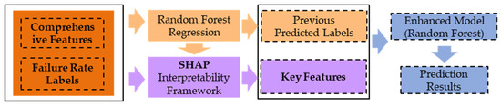
Figure 8.
Feature importance validation process.
Among these, the highly important features—identified as the top features following SHAP interpretability analysis and filtered by Figure 3—are selected from each cluster to form a partial feature set. The output results after training are presented in the Table 3.
Table 3.
Enhancing pre-stage and post-stage prediction results of the model.
Through Table 3, it is evident that there is a significant improvement in predictive performance following the enhancement of the model. This underscores the validity of the SHAP features, which contribute to increased model accuracy after the enhancement.
8. Model Validation
The feature extraction method and prediction model discussed in this paper were implemented in the marketing collection system of the grid company. Several stations, organized into batches, were identified as having high failure rates. The actual failures were recorded from field tests, as shown in the table below.
Through Table 4, it was found that the conclusions drawn are accurate. This demonstrates that the failure rate can be analyzed using the previously mentioned methodology and model predictions to obtain the actual failure rate, which can assist in identifying and rotating failure meters.
Table 4.
Commissioning and on-site collection of statistics.
9. Conclusions
This paper proposes a method for analyzing the status of group smart energy meters based on an interpretable random forest model. First, we utilize a knowledge graph for theoretical mechanism analysis, grouping and evaluating smart energy meters based on batch and the distribution network area. Subsequently, we analyze the extensive raw data corresponding to the grouped meters to extract state feature parameters related to three types of failures: verification-related, production-related, and deployment-related. This process generates a high-correlation feature dataset of power meter statuses along with their corresponding failure labels. We then analyze the relationship between the features and failure labels using a random forest model. Features are extracted for a specific research objective and input into the model to obtain the predicted failure probability. Conclusions from the state analysis are derived through SHAP interpretable analysis, and the model is refined based on these insights to enhance the accuracy of the output results. The state analysis method is validated using a substantial dataset, demonstrating the effectiveness of the group assessment approach. Comparative testing against other models shows the superior accuracy of ours. Additionally, the model undergoes SHAP interpretability analysis, which reveals the contribution of various feature parameters to the failure rate, thereby providing a foundation for the future maintenance of smart meters.
Future research will focus on expanding the model to industrial smart meters by incorporating features such as three-phase current imbalance, which are critical for non-residential scenarios. Additionally, it would be of great benefit to integrate real-time monitoring data, for example, 15 min interval metering data of electricity, current and voltage, to improve short-term failure prediction accuracy.
Author Contributions
Conceptualization, Z.W., Z.Z. (Zhengbo Zhang), W.W., Z.Z. (Zhen Zhang), X.X. and H.L.; Methodology, Z.W. and Z.Z. (Zhengbo Zhang); Software, Z.Z. (Zhengbo Zhang); Validation, W.W., Z.Z. (Zhen Zhang) and X.X.; Supervision, H.L.; Project administration, Z.W. and H.L.; Funding acquisition, Z.W. All authors have read and agreed to the published version of the manuscript.
Funding
This research was funded by State Grid Jiangsu Electric Power Co., Ltd. (Science and Technology Project) grant number J2024074. And The APC was funded by Marketing Service Center, State Grid Jiangsu Electric Power Co., Ltd.
Data Availability Statement
The original contributions presented in this study are included in the article. Further inquiries can be directed to the corresponding author.
Conflicts of Interest
Authors Zhongdong Wang, Weijiang Wu, Zhen Zhang and Xiaolin Xu were employed by the company State Grid Jiangsu Electric Power Co., Ltd. The remaining authors declare that the research was conducted in the absence of any commercial or financial relationships that could be construed as a potential conflict of interest.
References
- Zhang, L.P.; Hu, S.S.; Mei, N.; Li, R.X.; Xiao, X. Overview of research on reliability of smart meter. Electr. Meas. Instrum. 2020, 57, 134–140. [Google Scholar] [CrossRef]
- Machado, L.; Inga, E. Optimal Placement of UDAP in Advanced Metering Infrastructure for Smart Metering of Electrical Energy Based on Graph Theory. Electronics 2022, 11, 1767. [Google Scholar] [CrossRef]
- Garcés, H.O.; Godoy, J.; Riffo, G.; Sepúlveda, N.F.; Espinosa, E.; Ahmed, M.A. Development of an IoT-Enabled Smart Elec-tricity Meter for Real-Time Energy Monitoring and Efficiency. Electronics 2025, 14, 1173. [Google Scholar] [CrossRef]
- Liu, C. Research on Modeling of Fault Diagnosis and State Assessment of Electric Energy Metering Device. Master’s Thesis, Huazhong University of Science and Technology, Hubei, China, 2020. [Google Scholar]
- Lekshmana, R.; Padmanaban, S.; Mahajan, S.B.; Ramachandaramurthy, V.K.; Holm-Nielsen, J.B. Meter Placement in Power System Network—A Comprehensive Review, Analysis and Methodology. Electronics 2018, 7, 329. [Google Scholar] [CrossRef]
- Cheng, Y.Y.; Yang, H.X.; Xiao, J.; Wu, H.; Yao, C.G.; Li, C.X. Operation errors analysis of electric energy metering device and state evaluation method research. New Technol. Electr. Eng. Energy 2014, 33, 76–80. [Google Scholar] [CrossRef]
- Ma, H.M.; Li, Q.; Tao, P.; Shi, L.; Ma, X.T.; Feng, B. Research on the state perception technology of smart meters based on Bayesian and data-driven. Electr. Meas. Instrum. 2022, 59, 176–182, 188. [Google Scholar] [CrossRef]
- Chen, J.Y.; Zhong, C.C.; Peng, X.X.; Zhou, S.Y.; Zhou, J.; Zhang, Z.Y. Research on the Life Prediction Method of Meters Based on a Nonlinear Wiener Process. Electronics 2022, 11, 2026. [Google Scholar] [CrossRef]
- Xia, Z.; Zhang, J.A. Online Comprehensive Evaluation Method of State of Smart Energy Meters. Electr. Appl. Energy Effic. Manag. Technol. 2018, 21, 23–26. [Google Scholar] [CrossRef]
- Luo, Q.; Liu, C.Y.; Zhang, J.A.; Zhang, J.; Wang, S.K.; Ge, L.J. Online platform development and evaluation indexes of state inspection for smart meters. Electr. Meas. Instrum. 2017, 54, 94–99, 111. [Google Scholar] [CrossRef]
- Gao, S.Y.; An, T.; Song, J. Status evaluation of smart meter based on entropy weight-normal cloud model. Electr. Meas. Instrum. 2022, 59, 190–194. [Google Scholar] [CrossRef]
- Zhang, F.Z.; Liu, D.G.; Zhang, J.M.; Chen, W.; Li, X.Z. Design of a remote online evaluation system for electricity meters oriented toward multi-objective optimized proactive maintenance. Microcomput. Appl. 2024, 40, 76–79. [Google Scholar] [CrossRef]
- Lai, G.S. Data-driven online monitoring method for operational states of electricity meters. Electr. Meas. Instrum. 2023, 60, 193–200. [Google Scholar] [CrossRef]
- Yu, J.Z.; Xia, X.W.; Lei, C.J.; Zhao, L.D.; Ma, Q.; Chen, B.L. Prediction of electricity meter online rates using a support vector regression model optimized via Bayesian methods. Guangdong Electr. Power 2023, 36, 72–79. [Google Scholar] [CrossRef]
- Liu, Y.L. A Review of Random Forests. Master’s Thesis, Nankai University, Tianjin, China, 2008. Available online: https://d.wanfangdata.com.cn/thesis/Y1592135 (accessed on 31 March 2010).
- Li, P.Z.; Liu, L.Q.; Bo, Y.S. Anomalous electricity usage detection based on density subspace isolated forest. Sci. Technol. Eng. 2024, 24, 4115–4123. [Google Scholar] [CrossRef]
- Theil, H. Economics and Information Theory; North-Holland Publishing Company: Amsterdam, The Netherlands, 1967. [Google Scholar]
- Tao, J.; Zhang, L.T.; Zuo, Q.T.; Feng, Y.H.; Zhang, Y.S. Research on equity of water resources allocation based on Theil Index. Yangtze River 2023, 54, 113–119. [Google Scholar] [CrossRef]
- Lundberg, S.; Lee, S.I. A unified approach to interpreting model predictions. arXiv 2017, arXiv:1705.07874. [Google Scholar] [CrossRef]
- Alahakoon, D.; Yu, X. Smart electricity meter data intelligence for future energy systems: A survey. IEEE Trans. Ind. Inform. 2016, 12, 425–436. [Google Scholar] [CrossRef]
- Zhou, S.Y.; Wu, Z.H.; Chen, F.K.; Xie, Y.M.; Zhou, M.N.; Hu, X.P. Self-monitoring method for life of Watt-hour meter. Electr. Meas. Instrum. 2021, 58, 189–193. [Google Scholar] [CrossRef]
- GB/T 4798.3-2023; Classification of Environmental Conditions—Classification of Environmental Parameters and Their Severity—Part 3: Stationary Use at Weather-Protected Locations. State Administration for Market Regulation: Beijing, China, 2023.
- Wu, M.L. Salt spray in nature. Environ. Technol. 1993, 4, 3–8. [Google Scholar]
- Xu, G.B. Salt spray content and distribution in the coastal atmosphere of China. Environ. Technol. 1994, 3, 1–7. [Google Scholar]
- Zhu, J.; Liu, S.; Zhu, L.; Hu, A.; Zhao, Y.; Wang, Q.; Tang, Z.H.; Liu, J.H. Application of time clock synchronization in power information collection system. Electr. Meas. Instrum. 2016, 53, 157–159. [Google Scholar] [CrossRef]
- Chen, W. A Case Study of Big Data Audit Based on Visual Analysis Technology; Tongfang Knowledge Network (Beijing) Technology Co., Ltd.: Beijing, China, 2019; pp. 61–64. [Google Scholar] [CrossRef]
Disclaimer/Publisher’s Note: The statements, opinions and data contained in all publications are solely those of the individual author(s) and contributor(s) and not of MDPI and/or the editor(s). MDPI and/or the editor(s) disclaim responsibility for any injury to people or property resulting from any ideas, methods, instructions or products referred to in the content. |
© 2025 by the authors. Licensee MDPI, Basel, Switzerland. This article is an open access article distributed under the terms and conditions of the Creative Commons Attribution (CC BY) license (https://creativecommons.org/licenses/by/4.0/).